Non-equilibrium thermodynamics and Phase transition of Ehrenfest urns with interactions

The classic Ehrenfest model ehrenfest was introduced to solve the reversal and Poincare recurrence paradox huang ; poincare . It describes a total of $N$ particles in two urns that can randomly jump from one urn to the other with equal probability. The system has a Poincare cycle time of $2^{N}$ kac , providing a fundamental link between reversible microscopic dynamics and irreversible thermodynamics.

Later on, a directional jumping rate between urns was introduced siegert ; klein , and extensions to multi-urns kao03 ; nagler05 ; clark were made. Although there are various modifications nagler99 ; bouchaud ; boon ; lutsko ; schwammle ; shiino ; frank ; chavanis ; lipowski02a ; lipowski02b ; coppex ; shim of the classic Ehrenfest model, or even extensions by incorporating non-linear contribution casas ; curado ; nobre ; frank2005 , particles do not interact or the interaction is merely phenomenological. In fact, pairwise particle interaction in the same urn has been considered recently in the two-urn model cheng17 . The interacting two-urn Ehrenfest model can exhibit phase transitions by varying the interaction strength and directional jumping rate from which the relaxation time and Poincaré cycle can be derived. The multi-urn system with interaction and unbiased directional jumping will evolve to equilibrium and has been shown to exhibit different levels of non-uniformity emerge with the coexistence of uniform and non-uniform phases cheng20 . Contrary to the better understood equilibrium cases, non-equilibrium statistical physics remains challenging, partly due to the lack of well-characterised states. Even for non-equilibrium steady states (NESS), it is difficult to describe non-equilibrium phase transitions between different NESS and their relationship to some microscopic models. For example, selection rules, such as maximal or minimal entropy production principles nicolis ; MaxSbook ; Grandy have been proposed to determine the non-equilibrium states. Yet, universal guiding principles are still lacking.

In this manuscript, we consider urns with intra-urn interactions connected in a one-dimensional ring with directional jumping rates. We will show that the system has non-equilibrium steady states in uniform and non-uniform phases that can coexist. For high directional jumping rates with appropriate interaction strengths, the steady states become unstable. The phase diagram will be obtained analytically, and the relaxation dynamics to the NESS will be studied. The relationship between non-equilibrium thermodynamical variables, such as the internal entropy production rate, the rate of work done applied to the system, will be shown to obey a generalized thermodynamic law. Finally, we will demonstrate that, in the coexistence region, the internal entropy production rate fails to select the favorable steady state.

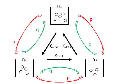
We consider three urns as illustrated in Fig.1 as this already captures the non-equilibrium physics. The state of the system is labeled by $\vec{n}=(n_{1},n_{2},n_{3})$ where $n_{i}$ is the number of particles in the $i$-th urn with $n_{1}+n_{2}+n_{3}=N$, the fixed total particle number. Similar to previous models cheng17 ; cheng20 , we include a pairwise attractive (repulsive) interaction with negative (positive) energy $J$ for particles in the same urn. Particles in different urns do not interact. A particle in the $i$-th urn (initial state $\vec{n}$) jumps to the $j$-th urn (final state $\vec{m}$) with corresponding transition probability

$\displaystyle T_{\vec{m},\vec{n}}$

$\displaystyle=$

$\displaystyle\frac{1}{{\rm e}^{-\frac{g}{N}(n_{i}-n_{j}-1)}+1}$

(1)

where $m_{i}=n_{i}-1$ and $m_{j}=n_{j}+1$. $g\equiv NJ\beta$ where $\beta$ is the inverse of effective temperature. Without interaction ($g=0$), we have $T_{\vec{m},\vec{n}}=\frac{1}{2}$. Next, a jumping rate is introduced such that the probability of anticlockwise (clockwise) direction is $p$ ($q$). For the sake of convenience, $p+q=1$ is imposed for which only changes the time scale.

After $s$ steps from the initial state, the probability of the state $\vec{n}$ is denoted by $\rho(\vec{n},s)$. The master equation from the $s$-th to the $(s+1)$-th time step can be written as

$\displaystyle\rho(\vec{n},s+1)-\rho(\vec{n},s)=\sum_{\vec{m}}(W_{\vec{n},\vec{m}}\rho(\vec{m},s)-W_{\vec{m},\vec{n}}\rho(\vec{n},s))$

(2)

where

$\displaystyle W_{\vec{m},\vec{n}}=\frac{n_{i}}{N}pT_{\vec{m},\vec{n}}$

(3)

holds if the particle jumps from the $i$-th to the $j$-th urn is anticlockwise, i.e., $(i,j)=(1,2),(2,3),(3,1)$, and

$\displaystyle W_{\vec{m},\vec{n}}=\frac{n_{i}}{N}qT_{\vec{m},\vec{n}}$

(4)

if $(i,j)=(2,1),(1,3),(3,2)$, which represents clockwise jumps.

Finally, the net particle flow rate from the $i$-th to the $j$-th urn (see Fig.1 for illustration) is given by

$\displaystyle K_{i\rightarrow j}(s)\equiv N\sum_{\vec{n}}(W_{\vec{m},\vec{n}}-W_{\vec{m}^{\prime},\vec{n}})\rho(\vec{n},s)$

(5)

where $m_{i}=n_{i}-1$, $m_{j}=n_{j}+1$, and $m^{\prime}_{i}=n_{i}+1$, $m^{\prime}_{j}=n_{j}-1$.

If $\lim_{s\rightarrow\infty}\rho(\vec{n},s)$ exists, it defines the steady state $\rho^{\rm ss}(\vec{n})$. Taking the limit $s\rightarrow\infty$ in Eq.(2) would lead to an equation in which $\rho^{\rm ss}(\vec{n})$ satisfies. No closed form exists in general. But for the case of $p=q=\frac{1}{2}$, an analytic expression for $\rho^{\rm ss}$ can be obtained

$\displaystyle\rho^{\rm ss}(\vec{n})=\frac{N!}{n_{1}!n_{2}!n_{3}!}{\rm e}^{-\frac{g}{2N}(n_{1}^{2}+n_{2}^{2}+n_{3}^{2})}$

(6)

up to a normalization constant. This steady state is also the equilibrium state, because it satisfies the condition of detailed balance

$\displaystyle W_{\vec{m},\vec{n}}\rho^{\rm ss}(\vec{n})=W_{\vec{n},\vec{m}}\rho^{\rm ss}(\vec{m})$

(7)

which can be verified by direct substitution. Results for the general case of $M$ urns at equilibrium can be found in Ref.cheng20 . For the three urns case here with the constraint $n_{1}+n_{2}+n_{3}=N$, one can define the population fraction with $x_{i}\equiv n_{i}/N$ and rewrite $\rho^{\rm ss}$ in terms of ${\vec{x}}\equiv(x_{1},x_{2})$ (two independent variables), $\rho^{\rm ss}(\vec{x})={\rm exp}\{Nf({\vec{x}})-\frac{1}{2}\log[(2\pi N)^{2}x_{1}x_{2}(1-x_{1}-x_{2})]+O(N^{-1})\}$ in large $N$ limit, where

	$\displaystyle f({\vec{x}})$	$\displaystyle=$	$\displaystyle-x_{1}\ln x_{1}-x_{2}\ln x_{2}$		(8)
			$\displaystyle-(1-x_{1}-x_{2})\ln(1-x_{1}-x_{2})$
			$\displaystyle-\frac{g}{2}(x_{1}^{2}+x_{2}^{2}+(1-x_{1}-x_{2})^{2})$

The saddle point approximation saddle gives asymptotic form

$\displaystyle\rho^{\rm ss}(\vec{x})\propto{\rm e}^{Nf(\vec{x}^{\rm sp})+\frac{N}{2}\sum_{i,j}\partial_{ij}f({\vec{x}}^{\rm sp})(x_{i}-x_{i}^{\rm sp})(x_{j}-x_{j}^{\rm sp})}$

(9)

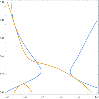
where ${\vec{x}}^{\rm sp}$ is the saddle point(s) satisfying $\partial_{1}f=\partial_{2}f=0$, $\partial_{11}f<0$, and $\partial_{11}f\partial_{22}f-(\partial_{12}f)^{2}>0$. This condition leads to

$\displaystyle x_{1}^{\rm sp}{\rm e}^{gx_{1}^{\rm sp}}=x_{2}^{\rm sp}{\rm e}^{gx_{2}^{\rm sp}}=x_{3}^{\rm sp}{\rm e}^{gx_{3}^{\rm sp}}$

(10)

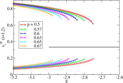
The solutions at different coupling constant $g$ are shown in the data of $p=0.5$ in Fig.2(a). The steady net particle flow at equilibrium from Eq.(5) reads

$\displaystyle\frac{K^{\rm ss}_{i\rightarrow j}}{N}$

$\displaystyle=$

$\displaystyle\frac{x_{i}^{\rm sp}{\rm e}^{gx_{i}^{\rm sp}}-x_{j}^{\rm sp}{\rm e}^{gx_{j}^{\rm sp}}}{2({\rm e}^{gx_{i}^{\rm sp}}+{\rm e}^{gx_{j}^{\rm sp}})}+O(1/N)$

(11)

which gives $K^{\rm ss}_{1\rightarrow 2}=K^{\rm ss}_{2\rightarrow 3}=K^{\rm ss}_{3\rightarrow 1}=0$ from Eq.(10), in large $N$ limit. At equilibrium, there is no net particle flow between any two urns. In addition, it is also easy to see from Eqs.(5) and (7) that for $p=q=\frac{1}{2}$, all fluxes $K^{\rm ss}_{i\rightarrow j}=0$ at equilibrium. On the other hand, or the non-equilibrium case of $p\neq q$, there can be non-vanishing circulating fluxes as in other general NESS systems aopingPNAS ; Chiang2017 ; Chang2021 .

So far, the recurrence relation in Eq.(2) cannot be solved analytically even for NESS. In this section, we will transform Eq.(2) into the Fokker-Planck equation. Let the (physical) time $t=\frac{\tau_{1}}{N}s$, where $\tau_{1}$ is the time scale of each single step from $s$ to $s+1$. Replace $\rho(\vec{n},s+1)-\rho(\vec{n},s)$ by $\rho(\vec{n},t+\frac{\tau_{1}}{N})-\rho(\vec{n},t)=\frac{\tau_{1}}{N}\frac{\partial\rho}{\partial t}+O((\frac{\tau_{1}}{N})^{2})$. Eq.(2) can be rewritten as

$\displaystyle\frac{\tau_{1}}{N}\frac{\partial\rho(\vec{n},t)}{\partial t}=\sum_{\vec{m}}(W_{\vec{n},\vec{m}}\rho(\vec{m},t)-W_{\vec{m},\vec{n}}\rho(\vec{n},t))$

(12)

Substituting Eqs.(1), (3)-(4) into Eq.(12) gives

			$\displaystyle\frac{\tau_{1}}{N}\frac{\partial\rho(\vec{x},t)}{\partial t}$		(13)
		$\displaystyle=$	$\displaystyle p\sum_{k=1}^{\infty}\frac{1}{k!N^{k}}\left(\frac{\partial}{\partial x_{1}}-\frac{\partial}{\partial x_{2}}\right)^{k}[\frac{x_{1}}{{\rm e}^{-g(x_{1}-x_{2})}+1}\rho(\vec{x},t)]$
			$\displaystyle+q\sum_{k=1}^{\infty}\frac{1}{k!N^{k}}\left(-\frac{\partial}{\partial x_{1}}+\frac{\partial}{\partial x_{2}}\right)^{k}[\frac{x_{2}}{{\rm e}^{g(x_{1}-x_{2})}+1}\rho(\vec{x},t)]$
			$\displaystyle+[\rm cyclic\ terms]$

which is known as the Kramers-Moyal expansion kramers ; moyal . From now on, we take $\tau_{1}=1$ for convenience.

If we further keep terms up to $O(1/N^{2})$, Eq.(13) becomes the Fokker-Planck equation

	$\displaystyle\frac{\partial\rho(\vec{x},t)}{\partial t}$	$\displaystyle=$	$\displaystyle-\sum_{i=1}^{2}\frac{\partial}{\partial x_{i}}[A_{i}(\vec{x})\rho(\vec{x};t)]$		(14)
			$\displaystyle+\frac{1}{2N}\sum_{i,j=1}^{2}\frac{\partial^{2}}{\partial x_{i}\partial x_{j}}[B_{ij}(\vec{x})\rho(\vec{x};t)]$

where

	$\displaystyle A_{1}(\vec{x})$	$\displaystyle=$	$\displaystyle-\frac{px_{1}}{{\rm e}^{-g(x_{1}-x_{2})}+1}+\frac{qx_{2}}{{\rm e}^{g(x_{1}-x_{2})}+1}-\frac{qx_{1}}{{\rm e}^{-g(2x_{1}+x_{2}-1)}+1}+\frac{p(1-x_{1}-x_{2})}{{\rm e}^{g(2x_{1}+x_{2}-1)}+1}$		(15)
	$\displaystyle A_{2}(\vec{x})$	$\displaystyle=$	$\displaystyle-\frac{qx_{2}}{{\rm e}^{-g(x_{2}-x_{1})}+1}+\frac{px_{1}}{{\rm e}^{g(x_{2}-x_{1})}+1}-\frac{px_{2}}{{\rm e}^{-g(2x_{2}+x_{1}-1)}+1}+\frac{q(1-x_{1}-x_{2})}{{\rm e}^{g(2x_{2}+x_{1}-1)}+1}$		(16)
	$\displaystyle B_{11}(\vec{x})$	$\displaystyle=$	$\displaystyle\frac{px_{1}}{{\rm e}^{-g(x_{1}-x_{2})+1}}+\frac{qx_{2}}{{\rm e}^{g(x_{1}-x_{2})}+1}+\frac{qx_{1}}{{\rm e}^{-g(2x_{1}+x_{2}-1)}+1}+\frac{p(1-x_{1}-x_{2})}{{\rm e}^{g(2x_{1}+x_{2}-1)}+1}$		(17)
	$\displaystyle B_{22}(\vec{x})$	$\displaystyle=$	$\displaystyle\frac{qx_{2}}{{\rm e}^{-g(x_{2}-x_{1})}+1}+\frac{px_{1}}{{\rm e}^{g(x_{2}-x_{1})}+1}+\frac{px_{2}}{{\rm e}^{-g(2x_{2}+x_{1}-1)}+1}+\frac{q(1-x_{1}-x_{2})}{{\rm e}^{g(2x_{2}+x_{1}-1)}+1}$		(18)
	$\displaystyle B_{12}(\vec{x})$	$\displaystyle=$	$\displaystyle B_{21}(\vec{x})=-\frac{px_{1}}{{\rm e}^{-g(x_{1}-x_{2})}+1}-\frac{qx_{2}}{{\rm e}^{g(x_{1}-x_{2})}+1}$		(19)

The WKB approximation wkb ; kubo ; dykman ; elgartv ; assaf yields the saddle points saddle ${\vec{x}}^{\rm sp}=(x_{1}^{\rm sp},x_{2}^{\rm sp})$ as

$$A_{1}({\vec{x}}^{\rm sp})=0,\quad A_{2}({\vec{x}}^{\rm sp})=0$$

(20)

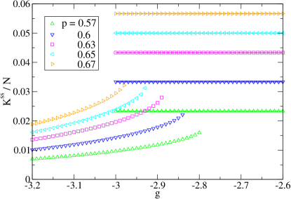
whose solutions at different $g$ and $p$ are shown in Fig.2. The physical meaning of Eq.(20) is that $K^{\rm ss}_{1\rightarrow 2}=K^{\rm ss}_{2\rightarrow 3}=K^{\rm ss}_{3\rightarrow 1}=K^{\rm ss}$, i.e., a constant non-zero cyclic flux of net particle along the ring which can be calculated from Eq.(5) as

$\displaystyle\frac{K^{\rm ss}}{N}$

$\displaystyle=$

$\displaystyle\frac{px_{1}^{\rm sp}{\rm e}^{gx_{1}^{\rm sp}}-qx_{2}^{\rm sp}{\rm e}^{gx_{2}^{\rm sp}}}{{\rm e}^{gx_{1}^{\rm sp}}+{\rm e}^{gx_{2}^{\rm sp}}}$

(21)

For uniform NESS ($x_{1}=x_{2}=\frac{1}{3}$), one obtains $K^{\rm ss}_{\rm u}={N\over 6}(p-q)$ and, for non-uniform NESS, $K^{\rm ss}_{\rm nu}$ can be computed using the non-uniform saddle point from Eqs.(20). The $K^{\rm ss}_{\rm u}$ and $K^{\rm ss}_{\rm nu}$ NESS fluxes as a function of $g$ at different $p$ are shown in Fig.3 indicating that the particle flux of the uniform NESS is always significantly larger than that of the non-uniform NESS. Notice that there is a coexistence region of uniform and non-uniform saddle points.

The NESS can be further analysed by expanding around the saddle point, i.e. using $A_{i}(\vec{x})\simeq\sum_{j}\partial_{j}A_{i}(\vec{x}^{\rm sp})(x_{j}-x_{j}^{\rm sp})\equiv\sum_{j}a_{ij}(x_{j}-x_{j}^{\rm sp})$ and $B_{ij}(\vec{x})\simeq B_{ij}(\vec{x}^{\rm sp})=b_{ij}$, the steady state particle distribution is

$\displaystyle\rho^{\rm ss}(\vec{x})\propto\exp[N\sum_{i,j=1}^{2}c_{ij}(x_{i}-x_{i}^{\rm sp})(x_{j}-x_{j}^{\rm sp})]$

(22)

where the matrix $\bf c$ is uniquely determined by the Lyapunov equations ${\bf a}{\bf c}^{-1}+{\bf c}^{-1}{\bf a}^{\rm t}=2{\bf b}$ (See Appendix A for details). The detailed balance condition can be transformed into ${\bf c}={\bf b}^{-1}{\bf a}$ (See Appendix B for details).

Obviously $x_{1}^{\rm sp}=x_{2}^{\rm sp}=x_{3}^{\rm sp}=\frac{1}{3}$ is always a saddle point of uniform population fraction. At this uniform NESS, we have

	$\displaystyle{\bf a}$	$\displaystyle=$	$\displaystyle-\frac{1}{2}\left(\begin{array}[]{cc}1+p+\frac{g}{2}&p-q\\ q-p&1+q+\frac{g}{2}\\ \end{array}\right)$		(25)
	$\displaystyle{\bf b}$	$\displaystyle=$	$\displaystyle\frac{1}{6}\left(\begin{array}[]{cc}2&-1\\ -1&2\\ \end{array}\right)$		(28)

which gives

$\displaystyle{\bf c}=-\frac{g+3}{2}\left(\begin{array}[]{cc}2&1\\ 1&2\\ \end{array}\right)$

(31)

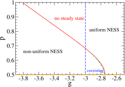
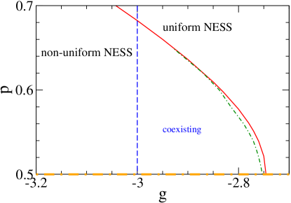
Hence its stability requires $g>-3$. The stable region for the non-uniform phase can be determined analytically in a similar manner and the results agree with the analytic ones of the phase boundary in Fig.4. In fact, the non-equilibrium physics of the system can be summarized by the phase diagram in Fig.4 whose phase boundaries can be determined analytically (see Appendix C for derivations). As the particle interaction is strongly repulsive (positively large $g$), the particles are uniformly distributed in every urn. On the other hand, the particles “prefer” to stay in the same urn (non-uniform distribution) if they are strongly attractive (negatively large $g$). In between, for low jumping rate, $1-p_{\rm s}<p<p_{\rm s}$ $(p_{\rm s}\simeq 0.6823)$, there is a coexistence region where both uniform and non-uniform distribution are locally stable. There is a first order non-equilibrium phase transition between the uniform and non-uniform NESSs whose transition value of $g$ can be determined from the analytic result of $K^{\rm ss}_{\rm u}$ and $K^{\rm ss}_{\rm nu}$ (see Appendix C for details) together with the results of mean steady state flux. The latter has to be determined numerically using (2) . The first order phase transition line (dashed-dotted curve) is also shown in Fig.4. It is close to the stability line of the non-uniform NESS (for magnification, see Fig.12 in Appendix C). As the jumping rate becomes higher, i.e. $p>p_{\rm s}$ (or $p<1-p_{\rm s}$), the system is far from equilibrium and steady states do no longer exist.

In this section, we studied how the system evolves to its steady states. When the system is initially away from its steady state, it will relax (thermalized) towards the nearby stable NESS whose dynamics near the NESS is determined by the eigenvalues of ${\bf a}$. From Eq.(14), and expand around the saddle point $\vec{x}^{\rm sp}$, we get the evolution of the average of particle numbers in the first and second urn as

$\displaystyle\frac{d}{dt}\left(\begin{array}[]{c}\langle x_{1}(t)\rangle\\ \langle x_{2}(t)\rangle\\ \end{array}\right)={\bf a}\left(\begin{array}[]{c}\langle x_{1}(t)\rangle-x_{1}^{\rm sp}\\ \langle x_{2}(t)\rangle-x_{2}^{\rm sp}\\ \end{array}\right)$

(36)

At uniform phase, $x_{1}^{\rm sp}=x_{2}^{\rm sp}=x_{3}^{\rm sp}=\frac{1}{3}$, its solution is

$\displaystyle\langle x_{1}(t)\rangle$

$\displaystyle=$

$\displaystyle\frac{1}{3}+\left\{(x_{1}(0)-\frac{1}{3})\cos(\frac{2\pi t}{\tau_{\rm osc}})-\frac{1}{\sqrt{3}}(x_{2}(0)-x_{3}(0))\sin(\frac{2\pi t}{\tau_{\rm osc}})\right\}{\rm e}^{-t/\tau_{\rm R}}$

(37)

describing the decaying process with oscillation, with the relaxation time

$\displaystyle\tau_{\rm R}=\frac{4}{g+3}$

(38)

and the oscillation period

$\displaystyle\tau_{\rm osc}=\frac{8\pi}{\sqrt{3}|p-q|}$

(39)

$x_{2}(t)$ and $x_{3}(t)$ can be obtained by making cyclic transformation to Eq.(37). Near equilibrium ($|p-q|\ll 1$), $\tau_{\rm osc}\gg\tau_{\rm R}$ , then the solution is simplified as

$\displaystyle\langle x_{i}(t)\rangle=\frac{1}{3}+(x_{i}(0)-\frac{1}{3}){\rm e}^{-t/\tau_{\rm R}}$

(40)

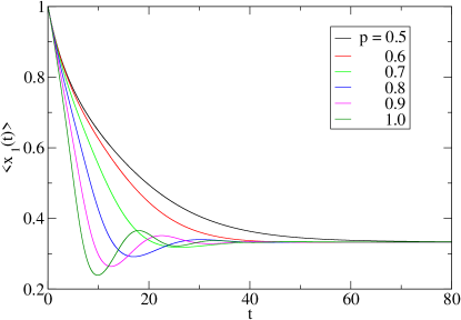
and the damped oscillation is not prominent. Fig.5 shows the relaxation towards the uniform NESS for different $p$, with $g=-2.5$ at which only the uniform NESS is stable. By increasing $p$ from 0.5 to 1.0, it can be seen from the direct numerical calculation by Eq.(2), starting from the non-uniform initial state $\vec{x}(0)=(1,0,0)$, the relaxation time keep almost unchanged and the oscillation in the occupation gradually appears.

When $g=-3.5$, the system stays at the non-uniform phase. To quantify the degree of non-uniformity, we define

$\displaystyle\psi\equiv\frac{1}{6}\langle(x_{1}-x_{2})^{2}+(x_{2}-x_{3})^{2}+(x_{3}-x_{1})^{2}\rangle$

(41)

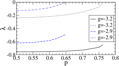
as the “non-uniformity” parameter cheng20 . It is almost zero for uniform phase and becomes larger for higher non-uniformity. The relaxation towards the non-uniform NESS is illustrated by $\psi(t)$ with $g=-3.5$ in Fig.6, showing a pure relaxation behavior. Starting from the uniform initial state $\vec{x}(0)=(\frac{1}{3},\frac{1}{3},\frac{1}{3})$, the system for different $p$ all relax to the non-uniform NESS and saturates at a high non-uniformity. This can be understood in terms of the eigenvalues of the matrix $\bf a$ at the non-uniform state which are always real and negative as shown in Fig.7.

We further examine the relationship between various thermodynamical quantities, first for general non-equilibrium states and then for the NESS cases. The Boltzmann (Gibbs, Shannon) entropy of the system is given by

$\displaystyle S=-\sum_{\vec{n}}\rho(\vec{n},t)\log\left(\rho(\vec{n},t)/\frac{N!}{n_{1}!n_{2}!n_{3}!}\right)$

(42)

where the multiplication factor $\frac{N!}{n_{1}!n_{2}!n_{3}!}$ is due to the degeneracy of $\rho(\vec{n},t)$ huang . Applying Eq.(2), the entropy production rate above can be written as

	$\displaystyle\frac{dS}{dt}$	$\displaystyle=$	$\displaystyle-\sum_{\vec{n},\vec{m}}(W_{\vec{n},\vec{m}}\rho(\vec{m},t)-W_{\vec{m},\vec{n}}\rho(\vec{n},t))\log\left(\rho(\vec{n},t)/\frac{N!}{n_{1}!n_{2}!n_{3}!}\right)$		(43)
		$\displaystyle=$	$\displaystyle\frac{N}{2}\sum_{\vec{n},\vec{m}}(W_{\vec{n},\vec{m}}\rho(\vec{m},t)-W_{\vec{m},\vec{n}}\rho(\vec{n},t))\log\left(\frac{W_{\vec{n},\vec{m}}\rho(\vec{m},t)}{W_{\vec{m},\vec{n}}\rho(\vec{n},t)}\right)$
			$\displaystyle+\frac{N}{2}\sum_{\vec{n},\vec{m}}(W_{\vec{n},\vec{m}}\rho(\vec{m},t)-W_{\vec{m},\vec{n}}\rho(\vec{n},t))\log\left(\frac{W_{\vec{m},\vec{n}}}{W_{\vec{n},\vec{m}}}\frac{\frac{N!}{n_{1}!n_{2}!n_{3}!}}{\frac{N!}{m_{1}!m_{2}!m_{3}!}}\right)$
		$\displaystyle=$	$\displaystyle\frac{d_{\rm i}S}{dt}+\frac{d_{\rm e}S}{dt}$

where the first term is the internal entropy production rate schnakenberg , which is positive-definite and only vanishes when the system is at equilibrium (Eq.(7)). It is the entropy produced during the irreversible process prigogine . The second term refers to the entropy production rate for the reversible process lebon into the system. In the following, we will show that

$\displaystyle\frac{d_{\rm e}S}{dt}=\beta\frac{dE}{dt}+\beta\frac{dW}{dt}$

(44)

where $\frac{dE}{dt}$ and $\frac{dW}{dt}$ are the rate of change of system energy and the rate of work done by the system, respectively. From the first law of thermodynamics (conservation law of energy), $Td_{\rm e}S$ can be identified as $dQ$, the heat flow to the system from the environment. In general, during thermalization process, $dS\geq\beta dQ=\beta dE+\beta dW$.

Using Eqs.(3)-(4), when the particle jumps from the $i$-th to the $j$-th urn, corresponding to the transition from state $\vec{n}$ to $\vec{m}$,

$\displaystyle\frac{W_{\vec{m},\vec{n}}}{W_{\vec{n},\vec{m}}}=\frac{p}{q}\frac{n_{i}}{n_{j}+1}{\rm e}^{\frac{g}{N}(n_{i}-n_{j}-1)}$

(45)

if the jump is in anti-clockwise direction. Otherwise, in clockwise direction,

$\displaystyle\frac{W_{\vec{m},\vec{n}}}{W_{\vec{n},\vec{m}}}=\frac{q}{p}\frac{n_{i}}{n_{j}+1}{\rm e}^{\frac{g}{N}(n_{i}-n_{j}-1)}$

(46)

Then

	$\displaystyle\frac{d_{\rm e}S}{dt}$	$\displaystyle=$	$\displaystyle\frac{N}{2}\sum_{\vec{n},\vec{m}}(W_{\vec{n},\vec{m}}\rho(\vec{m},t)-W_{\vec{m},\vec{n}}\rho(\vec{n},t))\frac{g}{N}(n_{i}-n_{j}-1)$		(47)
			$\displaystyle+\frac{N}{2}\sum_{\vec{n}}{\sum_{\vec{m}}}^{\rm ac}(W_{\vec{n},\vec{m}}\rho(\vec{m},t)-W_{\vec{m},\vec{n}}\rho(\vec{n},t))\log(\frac{p}{q})+\frac{N}{2}\sum_{\vec{n}}{\sum_{\vec{m}}}^{\rm c}(W_{\vec{n},\vec{m}}\rho(\vec{m},t)-W_{\vec{m},\vec{n}}\rho(\vec{n},t))\log(\frac{q}{p})$
		$\displaystyle=$	$\displaystyle\sum_{\vec{n},\vec{m}}g[n_{j}-(n_{i}-1)]W_{\vec{m},\vec{n}}\rho(\vec{n},t)-N\log(\frac{p}{q})\sum_{\vec{n}}{\sum_{\vec{m}}}^{\rm ac}(W_{\vec{m},\vec{n}}\rho(\vec{n},t)-W_{\vec{n},\vec{m}}\rho(\vec{m},t))$

where ac (c) stands for anti-clockwise (clockwise) direction. The first term is the rate of change of energy $\beta\frac{dE}{dt}$ and the second term is equal to the rate of work done which can be written as

$\displaystyle\beta\frac{dW}{dt}$

$\displaystyle=$

$\displaystyle-\beta\mu(K_{1\rightarrow 2}+K_{2\rightarrow 3}+K_{3\rightarrow 1})$

(48)

where $\mu\equiv\beta^{-1}\log(\frac{p}{q})$ is the effective chemical potential difference to actively drive the particle from one urn to another, and the natural boundary condition is assumed. Here Eq.(44) is proved, and hence a more general thermodynamic law

$$dS=d_{\rm i}S+\beta dE+\beta dW$$

(49)

is derived. Note that Eqs. (48) and (49) hold even for general non-equilibrium (non-steady state) processes.

For $p=q$, the system is at equilibrium and $\frac{dS}{dt}=\frac{d_{\rm i}S}{dt}=\frac{dQ}{dt}=\frac{dE}{dt}=\frac{dW}{dt}=0$. That is, all macroscopic thermodynamic quantities do not change with time. For $p\neq q$ under NESS, since the system energy and entropy are functionals of the probability distribution and hence are time independent, thus one has $\frac{dS}{dt}=\frac{dE}{dt}=0$. Using Eqs.(48)-(49),

$\displaystyle\frac{d_{\rm i}S}{dt}$

$\displaystyle=$

$\displaystyle-\beta\frac{dW}{dt}=-\beta\frac{dQ}{dt}=3K^{\rm ss}\log(\frac{p}{q})$

(50)

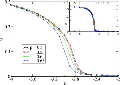
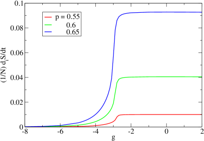
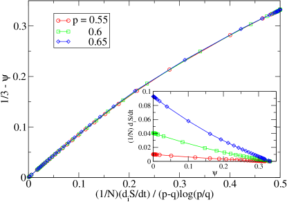
which is a positive constant, corresponding to the house-keeping heat production rate to maintain the NESS. All the work done ($-dW$) to the system is dissipated (measured by the internal EP $d_{\rm i}S$) into heat energy ($-dQ$). Furthermore, the more non-uniform is the NESS (Fig.8), the less is the particle flow (Fig.3), and hence the less internal EP (Fig.9). Since the internal EP for the non-uniform phase is always lower, the maximal EP principle could not be used to select the favorable state in the co-existence region. The first order non-equilibrium phase transition between the uniform and non-uniform NESS can also be observed by examining the internal EP rate as the particle attraction varies. Fig.9 shows a sharp drop near some threshold as $g$ decreases and signifying a first order transition from the high internal EP uniform NESS to the low internal EP non-uniform NESS. Interestingly, there is a connection between the internal EP rate and the non-uniformity in the NESS. As shown in Fig.10, when the relationship between $\frac{1}{3}-\psi^{\rm ss}$ and $\frac{1}{N}\frac{d_{\rm i}S}{dt}/(p-q)\log(\frac{p}{q})$ are plotted, all data with different $p$ are collapsed into a single curve. It implies the relation

$\displaystyle\left.\frac{d_{\rm i}S}{dt}\right|_{\rm ss}=N\Phi(\psi^{\rm ss})(p-q)\log(\frac{p}{q})$

(51)

where the function $\Phi(\psi^{\rm ss})$ is some decreasing function, i.e., $\Phi^{\prime}(\psi^{\rm ss})<0$. To have higher internal EP rates, the system should be more uniform (lower $\psi^{\rm ss}$), or with a higher direct jumping rate (higher $p$). Fig.10 agrees with the conjecture that more uniform states have higher EP.

In this paper, we extended the Ehrenfest urn model with interactions and directional jumps, allowing for detailed investigations of the non-equilibrium steady states and associated thermodynamics. We showed that the model provides different kinds of equilibrium and non-equilibrium states. Albeit simple the model may serve a convenient paradigm system to investigate a variety of statistical physics phenomena, ranging from equilibrium to NESS and even far from equilibrium situations.

In some situations, Landau type free energy can be constructed for NESS near a continuous phase transition haken ; Scipost or near the saddle-point(s) of NESS states aopingPNAS . However, it is still highly non-trivial to construct or establish the existence of NESS free energy in general, especially in our case of coexisting NESS related by first order transitions. On the other hand, because of the existence of probability density $\rho^{\rm ss}(\vec{x})$ at steady states, one may define the corresponding effective potential function $\Phi(\vec{x})=-\lim_{N\rightarrow\infty}\frac{1}{N}\log\rho^{\rm ss}(\vec{x})$. This NESS variable may reveals some NESS physical properties. Its numerical solution will be reported elsewhere.

At high direct jumping rate and moderate coupling constant, the system is far from equilibrium and cannot attain the steady state but limit cycle emerges instead. If the number of urns is more than three, chaotic behavior may be possible. Such models open the possibilities of investigating systems with different degree of non-equilibrium systematically. Detailed investigations will be reported elsewhere.

We express our gratitude to the anonymous referees for their suggestions on the improving the readability of the manuscript. The work was supported by the Ministry of Science and Technology of the Republic of China under grant no. 107-2112-M-008-013-MY3 and NCTS of Taiwan.

*

References

- (1) P. Ehrenfest and T. Ehrenfest, Uber zwei bekannte Einwande gegen das Boltzmannsche H-Theorem, Phys. Z. 8, 311 (1907).
- (2) K. Huang, Statistical Mechanics, 2nd ed. (Wiley, 1987).
- (3) H. Poincare, Sur le problème des trois corps et les équations de la dynamique, Acta Math. 13, 1 (1890).
- (4) M. Kac, Random Walk and the Theory of Brownian Motion, Am. Math. Mon. 54, 369 (1947).
- (5) A. J. F. Siegert, On the Approach to Statistical Equilibrium, Phys. Rev. 76, 1708 (1949).
- (6) M. J. Klein, Generalization of the Ehrenfest Urn Model, Phys. Rev. 103, 17 (1956).
- (7) Y. M. Kao and P. G. Luan, Poincare cycle of a multibox Ehrenfest urn model with directed transport, Phys. Rev. E67, 031101 (2003).
- (8) J. Nagler, Directed and undirected multiurn models in a one-dimensional ring, Phys. Rev. E72, 056129 (2005).
- (9) J. Clark, M. Kiwi, F. Torres, J. Rogan, and J.A. Valdivia, Generalization of the Ehrenfest urn model to a complex network, Phys. Rev. E92, 012103 (2015).
- (10) J. Nagler, C. Hauert, and H. G. Schuster, Self-organized criticality in a nutshell, Phys. Rev. E60, 2706 (1999).
- (11) J. P. Bouchaud and A. Georges, Anomalous diffusion in disordered media: statistical mechanics, models and physical applications, Phys. Rep. 195, 127 (1990).
- (12) J. P. Boon and J. F. Lutsko, Nonlinear diffusion from Einstein’s master equation, Europhys. Lett. 80, 60006 (2007).
- (13) J. F. Lutsko and J. P. Boon, Microscopic theory of anomalous diffusion based on particle interactions, Phys. Rev. E88, 022108 (2013).
- (14) V. Schwammle, F. D. Nobre, and E. M. F. Curado, Consequences of the H theorem from nonlinear Fokker-Planck equations, Phys. Rev. E76, 041123 (2007).
- (15) M. Shiino, Free energies based on generalized entropies and H-theorems for nonlinear Fokker–Planck equations, J. Math. Phys. 42, 2540 (2001).
- (16) T. D. Frank and A. Daffertshofer, H-theorem for nonlinear Fokker-Planck equations related to generalized thermostatistics, Phys. A 295, 455 (2001).
- (17) P. H. Chavanis, Generalized thermodynamics and Fokker-Planck equations: Applications to stellar dynamics and two-dimensional turbulence, Phys. Rev. E68, 036108 (2003).
- (18) A. Lipowski and M. Droz, Urn model of separation of sand, Phys. Rev. E65, 031307 (2002).
- (19) A. Lipowski and M. Droz, Moment ratios for an urn model of sand compartmentalization, Phys. Rev. E66, 016118 (2002).
- (20) F. Coppex, M. Droz, and A. Lipowski, Dynamics of the breakdown of granular clusters, Phys. Rev. E66, 011305 (2002).
- (21) G. M. Shim, B. Y. Park, and H. Lee, Analytic study of the urn model for separation of sand, Phys. Rev. E67, 011301 (2003).
- (22) G. A. Casas, F. D. Nobre, and E. M. F. Curado, Nonlinear Ehrenfest’s urn model, Phys. Rev. E91, 042139 (2015).
- (23) E. M. F. Curado and F. D. Nobre, Derivation of nonlinear Fokker-Planck equations by means of approximations to the master equation, Phys. Rev. E67, 021107 (2003).
- (24) F. D. Nobre, E. M. F. Curado, and G. Rowlands, A procedure for obtaining general nonlinear Fokker–Planck equations, Phys. A 334, 109 (2004).
- (25) T. D. Frank, Nonlinear Fokker-Planck Equations (Springer, 2005).
- (26) C. H. Tseng, Y. M. Kao, and C. H. Cheng, Ehrenfest urn model with interaction, Phys. Rev. E96, 032125 (2017).
- (27) C. H. Cheng, B. Gemao, and P. Y. Lai, Phase transitions in Ehrenfest urn model with interactions: Coexistence of uniform and nonuniform states, Phys. Rev. E101, 012123 (2020).
- (28) G. Nicolis and I. Prigogine, Self Organization in Non-equilibrium Systems (Wiley, 1977).
- (29) Entropy Measures, Maximum Entropy Principle and Emerging Applications, ed. Karmeshu, (Springer, New Delhi, 2003).
- (30) W. T. Grandy Jr., Entropy and the Time Evolution of Macroscopic Systems, (Oxford University Press, Oxford 2008).
- (31) In equilibrium statistical mechanics, when is large, in computing the partition function or any average physical variables, the method of steepest decent (one of the popular asymptotic methods) is applied. In this way, the physical varaibles we consider will be extended from real to complex plane. The ”optimal” point in this complex plane is not locally maximum or minimum, but a saddle point (Chapter 9 in Ref.[2]). This saddle point in the complex plane corresponds to the fixed point in the parameter space of the Fokker-Planck Equation in Eq.(14).
- (32) C. Kwon, P. Ao, and D. Thouless, Structure of stochastic dynamics near fixed points, PNAS 102, 13029 (2005).
- (33) K. H. Chiang, C. W. Chou, C. L. Lee, P. Y. Lai, and Y. F. Chen, Electrical autonomous Brownian gyrator, Phys. Rev. E 96, 032123 (2017).
- (34) H. Chang, C. L. Lee, P. Y. Lai, and Y. F. Chen, Autonomous Brownian gyrators: A study on gyrating characteristics, Phys. Rev. E 103, 022128 (2021).
- (35) H. A. Kramers, Brownian motion in a field of force and the diffusion model of chemical reactions, Physica 7, 284 (1940).
- (36) J. E. Moyal, Stochastic processes and statistical physics, J. Roy. Stat. Soc. B11, 150 (1949).
- (37) The WKB method is adopted in Section 6.6.7 from Ref.risken , which is the usual analytical method to solve the Fokker-Planck Equation with small diffusion coefficient (large limit in our case).
- (38) R. Kubo, K. Matsuo, and K. Kitahara, Fluctuation and relaxation of macrovariables, J. Stat. Phys. 9, 51 (1973).
- (39) M. I. Dykman, E. Mori, J. Ross, and P. M. Hunt, Large fluctuations and optimal paths in chemical kinetics, J. Chem. Phys. 100, 5735 (1994).
- (40) V. Elgartv and A. Kamenev, Rare event statistics in reaction-diffusion systems, Phys. Rev. E70, 041106 (2004).
- (41) M. Assaf and B. Meerson, WKB theory of large deviations in stochastic populations, J. Phys. A 50, 263001 (2017).
- (42) J. Schnakenberg, Network theory of microscopic and macroscopic behavior of master equation systems, Rev. Mod. Phys. 48, 571 (1976).
- (43) I. Prigogine, Non-Equilibrium Statistical Mechanics (Dover, 2017).
- (44) G. Lebon, D. Jou, and J. Casas-Vazquez, Understanding Non-equilibrium Thermodynamics.Foundations, Applications, Frontiers (Springer, Berlin 2007).
- (45) H. Haken, Information and Self-Organization, A Macroscopic Approach to Complex Systems (Springer, 1988).
- (46) C. Aron and C. Chamon, Landau theory for non-equilibrium steady states, SciPost Phys. 8, 074 (2020).
- (47) M. C. Wang and G. E. Uhlenbeck, On the Theory of the Brownian Motion II, Rev. Mod. Phys. 17, 323 (1945).
- (48) H. Risken, The Fokker-Planck Equation (Springer, 1983).