Non-Drude behaviour of optical conductivity in Kondo-lattice systems

In the Drude model, optical conductivity is given by [1]

$\displaystyle\sigma(\omega)=\frac{ne^{2}}{m}\frac{1}{i\omega+\frac{1}{\tau_{D}}}.$

(1)

here $\tau_{D}$ is the Drude scattering rate. The real and imaginary parts of the conductivity are given by

$$\sigma^{\prime}(\omega)=\frac{ne^{2}}{m}\frac{\frac{1}{\tau_{D}}}{\omega^{2}+(\frac{1}{\tau_{D}})^{2}}.$$

(2)

$$\sigma^{\prime\prime}(\omega)=\frac{ne^{2}}{m}\frac{\omega}{\omega^{2}+(\frac{1}{\tau_{D}})^{2}}.$$

(3)

In the high frequency limit $\omega\gg\frac{1}{\tau_{D}}$, the real part of conductivity scales $\sigma^{\prime}(\omega)\sim\frac{1}{\omega^{2}}$. This is a typical signature of "good" metals [1, 2]. But it has been experimentally observed that $\sigma^{\prime}(\omega)$ scales as $\frac{1}{\omega}$ or some fractional power of $\frac{1}{\omega}$ in many situations (such as in the "normal" state of high temperature superconductors).The metallic states which show such a behaviour are called strange metals [3]

The aim of the present work is to show that the behaviour $\sigma^{\prime}(\omega)\sim\frac{1}{\omega}$ can arise in a situation where electron scattering happens via magnetic spin fluctuations, whereas the standard electron-impurity and electron-phonon scaterring lead to the Drude behaviour ($\sigma^{\prime}(\omega)\sim\frac{1}{\omega^{2}}$).

In simple Drude model a frequency independent time $\tau_{D}$ governs the relaxation of current and $\frac{1}{\tau_{D}}$ is identified as the Drude scattering rate. The simple Langevin equation leads to [2, 3, 4]

$$\sigma(\omega)=\frac{ne^{2}}{m}\frac{1}{i\omega+\frac{1}{\tau_{D}}}$$

(4)

Here $n$ and $m$ are the number density and mass of the free electrons. The standard Drude formula has many limitations [4]. The Generalized Drude Formula (GDF) writes the dynamical conductivity in terms of the memory function[2, 3, 4]

$$\sigma(\omega)=\frac{ne^{2}}{m}\frac{1}{i\omega+M(\omega)}.$$

(5)

where $M(\omega)$ is the complex frequency dependent memory function. In some situations when $M(\omega)$ becomes the frequency independent, the generalized Drude formula (5) reduces to simple Drude formula(4) [2, 3, 4].

I take the $s$-$d$ Hamiltonian (known as Kondo-lattice Hamiltonian) for explicit calculations, and compute the imaginary part of the memory function. The Kondo-lattice Hamiltonian is given by

$\displaystyle H_{sd}$

$\displaystyle=$

$\displaystyle\frac{J}{N}\sum_{k^{\prime}k}\bigg{\{}c^{\dagger}_{k^{\prime}\uparrow}c_{k\downarrow}S^{-}(k^{\prime}-k)+c^{\dagger}_{k^{\prime}\downarrow}c_{k\uparrow}S^{+}(k^{\prime}-k)+(c^{\dagger}_{k^{\prime}\uparrow}c_{k\uparrow}-c^{\dagger}_{k^{\prime}\downarrow}c_{k\downarrow})S^{z}(k^{\prime}-k)\bigg{\}}$

(9)

here $J$ is coupling constant between $s$-electron and $d$ electrons [5]. $c^{\dagger}$ and $c$ are the creation and annihilation operators for $s$-electrons. $S^{-}(k^{\prime}-k)$ and $S^{+}(k^{\prime}-k)$ are the spin lowering and spin raising operator of $d$ or $f$ electrons and these are given as

$\displaystyle S^{-}(q)=\sum_{k}a^{*}_{k+q\downarrow}a_{k\uparrow},~{}~{}~{}~{}~{}~{}~{}~{}~{}S^{+}(q)=\sum_{k}a^{*}_{k+q\uparrow}a_{k\downarrow}.$

(10)

Under the assumption of weak coupling (electron K.E.$\gg J$) between the $s$ and $d$ electrons the Wölfle-Götze equation of motion method defines the memeory function as [5, 6, 7, 8]

$\displaystyle M(z)\simeq\frac{1}{z}(\frac{m}{ne^{2}})[\langle\langle\dot{J_{1}};\dot{J_{1}}\rangle\rangle_{z}-\langle\langle\dot{J_{1}};\dot{J_{1}}\rangle\rangle_{0}].$

(11)

where $\dot{J_{1}}=-\frac{i}{\hbar}[J_{1},H_{sd}]$. $J_{1}=\frac{1}{V}\sum_{k\sigma}ev_{k}c^{\dagger}_{k\sigma}c_{k\sigma}$ is the current density operator and $V$ is volume of the sample. I define the current-current correlator as $\phi(z)=\langle\langle\dot{J_{1}};\dot{J_{1}}\rangle\rangle$ and compute the correlator in terms of fermi functions of electrons(for more details refer to [5]), we get

	$\displaystyle\phi(z)$	$\displaystyle=$	$\displaystyle-\frac{e^{2}J^{2}}{N^{2}\hbar^{3}V}\sum_{k^{\prime}k}(v_{1}(k^{\prime})-v_{1}(k))^{2}\bigg{\{}f^{s}_{k^{\prime}}(1-f^{s}_{k})\sum_{k_{d},k^{\prime}_{d}}(f^{d}_{k_{d}}-f^{d}_{k^{\prime}_{d}})-(f^{s}_{k}-f^{s}_{k^{\prime}})$		(12)
			$\displaystyle\sum_{k_{d},k^{\prime}_{d}}f^{d}_{k_{d}}(1-f^{d}_{k^{\prime}_{d}})\bigg{\}}~{}\bigg{[}\frac{1}{\frac{\epsilon_{k^{\prime}}}{\hbar}-\frac{\epsilon_{k}}{\hbar}-\omega_{k^{\prime}-k}+z}+\frac{1}{\frac{\epsilon_{k^{\prime}}}{\hbar}-\frac{\epsilon_{k}}{\hbar}-\omega_{k^{\prime}-k}-z}\bigg{]}.$

On substituting the expression (12) in (11) the frequency depedent memory function can be expressed as

	$\displaystyle M(z)$	$\displaystyle=$	$\displaystyle-\frac{J^{2}m}{N^{2}\hbar^{3}nV\omega}\sum_{k^{\prime}k}(v_{1}(k^{\prime})-v_{1}(k))^{2}\bigg{\{}f^{s}_{k^{\prime}}(1-f^{s}_{k})\sum_{k_{d},k^{\prime}_{d}}(f^{d}_{k_{d}}-f^{d}_{k^{\prime}_{d}})-(f^{s}_{k}-f^{s}_{k^{\prime}})$		(13)
			$\displaystyle\sum_{k_{d},k^{\prime}_{d}}f^{d}_{k_{d}}(1-f^{d}_{k^{\prime}_{d}})\bigg{\}}\bigg{[}\frac{1}{\frac{\epsilon_{k^{\prime}}}{\hbar}-\frac{\epsilon_{k}}{\hbar}-\omega_{k^{\prime}-k}+z}+\frac{1}{\frac{\epsilon_{k^{\prime}}}{\hbar}-\frac{\epsilon_{k}}{\hbar}-\omega_{k^{\prime}-k}-z}$
			$\displaystyle~{}~{}~{}~{}~{}~{}~{}~{}~{}~{}~{}~{}~{}-\frac{1}{\frac{\epsilon_{k^{\prime}}}{\hbar}-\frac{\epsilon_{k}}{\hbar}-\omega_{k^{\prime}-k}}-\frac{1}{\frac{\epsilon_{k^{\prime}}}{\hbar}-\frac{\epsilon_{k}}{\hbar}-\omega_{k^{\prime}-k}}\bigg{]},$

here we write the short notation for $f^{1}_{d}(q)=\sum_{k_{d},k^{\prime}_{d}}(f^{d}_{k_{d}}-f^{d}_{k^{\prime}_{d}})$ and $f^{1}_{d}(q)=\sum_{k_{d},k^{\prime}_{d}}f^{d}_{k_{d}}(1-f^{d}_{k^{\prime}_{d}})$. From the above expression the imginary part of the memory function can be written as (for more details refer to ref. [5])

$$M^{\prime\prime}(\omega)=\frac{1}{12\pi^{3}}\frac{J^{2}Vm^{2}}{N^{2}\hbar^{6}nq^{2}_{s}}\int_{0}^{q_{D}}dqq^{3}\bigg{[}\int_{0}^{\infty}d\epsilon\sqrt{\epsilon}\times\\ \bigg{(}\underbrace{\frac{\sqrt{\epsilon+\hbar\omega_{q}-\hbar\omega}f^{s}(\epsilon+\hbar\omega_{q}-\hbar\omega)-\sqrt{\epsilon+\hbar\omega_{q}+\hbar\omega}f^{s}(\epsilon+\hbar\omega_{q}+\hbar\omega)}{\omega}}_{\mathfrak{T}_{1}}\bigg{)}\\ ~{}\times(1-f^{s}(\epsilon))f^{1}_{d}(q)+\int_{0}^{\infty}d\epsilon\sqrt{\epsilon}\bigg{(}\underbrace{\frac{\sqrt{\epsilon+\hbar\omega_{q}+\hbar\omega}-\sqrt{\epsilon+\hbar\omega_{q}-\hbar\omega}}{\omega}}_{\mathfrak{T}_{2}}\bigg{)}\times\\ f^{s}(\epsilon)f^{2}_{d}(q)+\int_{0}^{\infty}\frac{d\epsilon\sqrt{\epsilon}}{\omega}\bigg{(}\sqrt{\epsilon+\hbar\omega_{q}-\hbar\omega}f^{s}(\epsilon+\hbar\omega_{q}-\hbar\omega)-~{}~{}~{}~{}~{}~{}\\ ~{}\sqrt{\epsilon+\hbar\omega_{q}+\hbar\omega}f^{s}(\epsilon+\hbar\omega_{q}+\hbar\omega)\bigg{)}f^{2}_{d}(q)\bigg{]}.~{}~{}~{}~{}~{}$$

(14)

In the next section I compute the frequency dependent part of the memory function under the assumption of the long wavelength limit.

I assume that momentum randomization of $s$-electrons happens via the creation of magnetic spin waves in the sub-system of $d$-electrons. This is the mechanism of resistivity in the considered setting. In equation (14) $\hbar\omega_{q}$ is the energy of the magnetic spin waves. One takes $\hbar\omega_{q}=c_{m}q^{2}$, where $c_{m}$ is a constant. I further assumes that ($\hbar\omega_{q_{D}}\ll\mu_{s}$). That is the maximum energy of magnetic spin waves is much less than the chemical potential of $s$-electrons. Under these assumptions terms $\mathfrak{T}_{1}$ and $\mathfrak{T}_{2}$ in equation (14) can be approximated as :

$$\mathfrak{T}_{1}\simeq\frac{\sqrt{\epsilon-\hbar\omega}}{e^{\beta(\epsilon-\hbar\omega-\mu_{s})}+1}-\frac{\sqrt{\epsilon+\hbar\omega}}{e^{\beta(\epsilon+\hbar\omega-\mu_{s})}+1}+\frac{q^{2}c_{m}}{2}\bigg{(}\frac{1}{\sqrt{\epsilon-\hbar\omega}(1+e^{\beta(\epsilon-\hbar\omega-\mu_{s})})}\\ ~{}~{}~{}~{}-\frac{1}{\sqrt{\epsilon+\hbar\omega}(1+e^{\beta(\epsilon+\hbar\omega-\mu_{s})})}-2\beta\frac{\sqrt{\epsilon-\hbar\omega}e^{\beta(\epsilon-\hbar\omega-\mu_{s})}}{(1+e^{\beta(\epsilon-\hbar\omega-\mu_{s})})^{2}}+2\beta\frac{\sqrt{\epsilon+\hbar\omega}e^{\beta(\epsilon+\hbar\omega-\mu_{s})}}{(1+e^{\beta(\epsilon+\hbar\omega-\mu_{s})})^{2}}\bigg{)}+O(q^{4}).~{}~{}~{}~{}~{}~{}$$

(15)

$\displaystyle\mathfrak{T}_{2}$

$\displaystyle\simeq$

$\displaystyle\sqrt{\epsilon+\hbar\omega}-\sqrt{\epsilon-\hbar\omega}+\frac{q^{2}c_{m}}{2}\bigg{(}\frac{1}{\sqrt{\epsilon+\hbar\omega}}-\frac{1}{\sqrt{\epsilon-\hbar\omega}}\bigg{)}+O(q^{4}).$

On Substituting expanded form of the terms $\mathfrak{T}_{1}$ and $\mathfrak{T}_{2}$ in expression (14), we obtain

$$M^{\prime\prime}(\omega)=\frac{J^{2}Vm^{2}}{12\pi^{3}N^{2}\hbar^{6}nq^{2}_{s}}\int_{0}^{q_{D}}dqq^{3}\bigg{[}\int_{0}^{\infty}\frac{d\epsilon\sqrt{\epsilon}}{\omega}\bigg{\{}\frac{\sqrt{\epsilon-\hbar\omega}}{(1+e^{\beta(\epsilon-\hbar\omega-\mu_{s})})}-\frac{\sqrt{\epsilon+\hbar\omega}}{(1+e^{\beta(\epsilon+\hbar\omega-\mu_{s})})}+\\ ~{}\frac{q^{2}c_{m}}{2}\bigg{(}\frac{(\sqrt{\epsilon-\hbar\omega})^{-1}}{(1+e^{\beta(\epsilon-\hbar\omega-\mu_{s})})}-\frac{(\sqrt{\epsilon+\hbar\omega})^{-1}}{(1+e^{\beta(\epsilon+\hbar\omega-\mu_{s})})}-2\beta\frac{\sqrt{\epsilon-\hbar\omega}e^{\beta(\epsilon-\hbar\omega-\mu_{s})}}{(1+e^{\beta(\epsilon-\hbar\omega-\mu_{s})})^{2}}+2\beta\frac{\sqrt{\epsilon+\hbar\omega}e^{\beta(\epsilon+\hbar\omega-\mu_{s})}}{(1+e^{\beta(\epsilon+\hbar\omega-\mu_{s})})^{2}}\bigg{)}+~{}\\ ~{}~{}O(q^{4})\bigg{\}}(1-f^{s}(\epsilon))f^{1}_{d}(q)+\int_{0}^{\infty}\frac{d\epsilon\sqrt{\epsilon}}{\omega}\bigg{\{}\sqrt{\epsilon+\hbar\omega}-\sqrt{\epsilon-\hbar\omega}+\frac{q^{2}c_{m}}{2}\bigg{(}\frac{1}{\sqrt{\epsilon+\hbar\omega}}-\frac{1}{\sqrt{\epsilon-\hbar\omega}}\bigg{)}\bigg{\}}~{}\\ ~{}f^{s}(\epsilon)f^{2}_{d}(q)+\int_{0}^{\infty}\frac{d\epsilon\sqrt{\epsilon}}{\omega}\bigg{\{}\frac{\sqrt{\epsilon-\hbar\omega}}{(1+e^{\beta(\epsilon-\hbar\omega-\mu_{s})})}-\frac{\sqrt{\epsilon+\hbar\omega}}{(1+e^{\beta(\epsilon+\hbar\omega-\mu_{s})})}+\frac{q^{2}c_{m}}{2}\bigg{(}\frac{(\sqrt{\epsilon-\hbar\omega})^{-1}}{(1+e^{\beta(\epsilon-\hbar\omega-\mu_{s})})}-~{}\\ ~{}\frac{(\sqrt{\epsilon+\hbar\omega})^{-1}}{(1+e^{\beta(\epsilon+\hbar\omega-\mu_{s})})}-2\beta\frac{\sqrt{\epsilon-\hbar\omega}e^{\beta(\epsilon-\hbar\omega-\mu_{s})}}{(1+e^{\beta(\epsilon-\hbar\omega-\mu_{s})})^{2}}+2\beta\frac{\sqrt{\epsilon+\hbar\omega}e^{\beta(\epsilon+\hbar\omega-\mu_{s})}}{(1+e^{\beta(\epsilon+\hbar\omega-\mu_{s})})^{2}}\bigg{)}+O(q^{4})\bigg{\}}f^{2}_{d}(q,\epsilon_{d})\bigg{]},~{}~{}~{}~{}~{}~{}~{}~{}~{}~{}~{}~{}$$

(17)

my next task is to perform $q$ integration in the expression (17). The terms $f^{1}_{d}(q)$ and $f^{2}_{d}(q)$ also contribute $q$ terms in the integrals. The expansion of $f^{1}_{d}(q)=\sum_{k_{d}}[f^{d}(\epsilon_{k_{d}})-f^{d}(\epsilon_{k^{\prime}_{d}})]$ in long wavelength limit ($q\rightarrow 0$) gives

$\displaystyle f^{1}_{d}(q)$

$\displaystyle=$

$\displaystyle\sum_{k_{d}}[f^{d}(\epsilon_{k_{d}})-f^{d}(\epsilon_{k_{d}})-q\frac{\partial f^{d}(\epsilon_{k^{\prime}_{d}})}{\partial q}|_{q=0}-\frac{q^{2}}{2!}\frac{\partial^{2}f^{d}(\epsilon_{k^{\prime}_{d}})}{\partial q^{2}}|_{q=0}-\frac{q^{3}}{3!}\frac{\partial^{3}f^{d}(\epsilon_{k^{\prime}_{d}})}{\partial q^{3}}|_{q=0}..].$

On converting summation into integrals ($\sum_{k_{d}}=\frac{V}{(2\pi)^{3}}\int d^{3}k_{d}$), we get

	$\displaystyle f^{1}_{d}(q)$	$\displaystyle=$	$\displaystyle-\frac{V}{(2\pi)^{2}}\int_{0}^{\infty}k^{2}_{d}dk_{d}\int_{0}^{\pi}\sin\theta d\theta\bigg{[}q\frac{\partial f^{d}(\epsilon_{k^{\prime}_{d}})}{\partial q}|_{q=0}+\frac{q^{2}}{2!}\frac{\partial^{2}f^{d}(\epsilon_{k^{\prime}_{d}})}{\partial q^{2}}|_{q=0}$		(19)
			$\displaystyle~{}~{}~{}~{}~{}~{}~{}~{}~{}~{}~{}~{}~{}~{}~{}~{}~{}+\frac{q^{3}}{3!}\frac{\partial^{3}f^{d}(\epsilon_{k^{\prime}_{d}})}{\partial q^{3}}|_{q=0}.......\bigg{]}.$

Further simplification of $f^{1}_{d}(q)$, we obtain (for more details refer to [5])

$$f^{1}_{d}(\epsilon_{d},q)=V\frac{q^{2}}{4\pi^{2}}\frac{\sqrt{2m_{d}}}{\hbar}\bigg{[}\beta\int_{0}^{\infty}\frac{d\epsilon_{d}\sqrt{\epsilon_{d}}e^{\beta(\epsilon_{d}-\mu_{d})}}{(e^{\beta(\epsilon_{d}-\mu_{d})}+1)^{2}}+\frac{2}{3}\beta^{2}\int_{0}^{\infty}\frac{d\epsilon_{d}\epsilon_{d}^{\frac{3}{2}}e^{\beta(\epsilon_{d}-\mu_{d})}}{(e^{\beta(\epsilon_{d}-\mu_{d})}+1)^{2}}-\\ ~{}~{}~{}~{}~{}~{}~{}~{}~{}~{}~{}~{}~{}~{}\frac{4}{3}\beta^{2}\int_{0}^{\infty}\frac{d\epsilon\epsilon^{\frac{3}{2}}e^{2\beta(\epsilon_{d}-\mu_{d})}}{(e^{\beta(\epsilon_{d}-\mu_{d})}+1)^{3}}\bigg{]}.$$

(20)

Let $m_{d}$ be the mass of the $d$-electrons and m is the mass of $s$-electrons, introduces $m_{d}=m\lambda$ and set $\sqrt{2m\mu_{s}}=\hbar q_{s}$ The expression $f^{1}_{d}(\epsilon_{d})$ can be written as

$$f^{1}_{d}(\epsilon_{d},q)=Vq_{s}\frac{q^{2}}{4\pi^{2}}\sqrt{\frac{\lambda}{\beta\mu_{s}}}\bigg{(}\int_{-\beta\mu_{d}}^{\infty}\frac{dx\sqrt{x+\beta\mu_{d}}e^{x}}{(e^{x}+1)^{2}}+\frac{2}{3}\int_{-\beta\mu_{d}}^{\infty}\frac{dx(x+\beta\mu_{d})^{\frac{3}{2}}e^{x}}{(e^{x}+1)^{2}}-\\ ~{}~{}\frac{4}{3}\int_{-\beta\mu_{d}}^{\infty}\frac{dx(x+\beta\mu_{d})^{\frac{3}{2}}e^{2x}}{(e^{x}+1)^{3}}\bigg{)},~{}~{}~{}~{}~{}~{}~{}$$

(21)

and on the similiar lines the $f^{2}_{d}(\epsilon_{d},q)$ expression gives

$$f^{2}_{d}(\epsilon_{d},q)=\frac{Vq^{3}_{s}~{}}{4\pi^{2}}(\frac{\lambda}{\beta\mu_{s}})^{\frac{3}{2}}\int_{-\beta\mu_{d}}^{\infty}\frac{dx\sqrt{x+\beta\mu_{d}}e^{x}}{(e^{x}+1)^{2}}+\frac{Vq_{s}q^{2}}{4\pi^{2}}\sqrt{\frac{\lambda}{\beta\mu_{s}}}\\ ~{}\bigg{(}\int_{-\beta\mu_{d}}^{\infty}\frac{dx\sqrt{x+\beta\mu_{d}}e^{x}}{(e^{x}+1)^{3}}+\frac{2}{3}\int_{-\beta\mu_{d}}^{\infty}\frac{dx(x+\beta\mu_{d})^{\frac{3}{2}}e^{x}}{(e^{x}+1)^{3}}-\frac{4}{3}\int_{-\beta\mu_{d}}^{\infty}\frac{dx(x+\beta\mu_{d})^{\frac{3}{2}}e^{2x}}{(e^{x}+1)^{4}}\bigg{)}.~{}~{}~{}~{}~{}$$

(22)

On substitution the simplified form of the expressions $f^{1}_{d}(\epsilon_{d},q)$ and $f^{2}_{d}(\epsilon_{d},q)$ from equation (21) and (22) in the expression (17) and computing $q$ integral, we get

$$M^{\prime\prime}(\omega)=\frac{J^{2}Vm^{2}}{12\pi^{3}N^{2}\hbar^{8}n}\bigg{[}\sqrt{\frac{\lambda}{\beta\mu_{s}}}\int_{0}^{\infty}\frac{d\epsilon\sqrt{\epsilon}}{\omega}\bigg{(}(\frac{q_{D}}{q_{s}})^{6}\frac{q^{5}_{s}}{6}h_{1}(\epsilon,\hbar\omega)+(\frac{q_{D}}{q_{s}})^{8}\frac{c_{m}q^{7}_{s}}{16}h_{2}(\epsilon,\hbar\omega)\bigg{)}\\ \times(1-f^{s}(\epsilon))\Xi(\beta\mu_{d})+(\frac{\lambda}{\beta\mu_{s}})^{\frac{3}{2}}\int_{0}^{\infty}\frac{d\epsilon\sqrt{\epsilon}}{\omega}\bigg{(}(\frac{q_{D}}{q_{s}})^{4}\frac{q^{5}_{s}}{4}h_{3}(\epsilon,\hbar\omega)+(\frac{q_{D}}{q_{s}})^{6}\frac{c_{m}q^{7}_{s}}{12}h_{4}(\epsilon,\hbar\omega)\bigg{)}f^{s}(\epsilon)\\ ~{}\Xi_{1}(\beta\mu_{d})+~{}\sqrt{\frac{\lambda}{\beta\mu_{s}}}\int_{0}^{\infty}\frac{d\epsilon\sqrt{\epsilon}}{\omega}\bigg{(}(\frac{q_{D}}{q_{s}})^{6}\frac{q^{5}_{s}}{6}h_{3}(\epsilon,\hbar\omega)+(\frac{q_{D}}{q_{s}})^{8}\frac{c_{m}q^{7}_{s}}{16}h_{4}(\epsilon,\hbar\omega)\bigg{)}f^{s}(\epsilon)\Xi_{2}(\beta\mu_{d})+\\ ~{}(\frac{\lambda}{\beta\mu_{s}})^{\frac{3}{2}}\times\int_{0}^{\infty}\frac{d\epsilon\sqrt{\epsilon}}{\omega}\bigg{(}(\frac{q_{D}}{q_{s}})^{4}\frac{q^{5}_{s}}{4}h_{1}(\epsilon,\hbar\omega)+(\frac{q_{D}}{q_{s}})^{6}\frac{c_{m}q^{5}_{s}}{12}h_{2}(\epsilon,\hbar\omega)\bigg{)}\Xi_{1}(\beta\mu_{d})+~{}~{}\\ ~{}\sqrt{\frac{\lambda}{\beta\mu_{s}}}\times\int_{0}^{\infty}\frac{d\epsilon\sqrt{\epsilon}}{\omega}\bigg{(}(\frac{q_{D}}{q_{s}})^{6}\frac{q^{5}_{s}}{6}h_{1}(\epsilon,\hbar\omega)+(\frac{q_{D}}{q_{s}})^{8}\frac{c_{m}q^{7}_{s}}{16}h_{2}(\epsilon,\hbar\omega)\bigg{)}\Xi_{2}(\beta\mu_{d})\bigg{]}.~{}~{}~{}~{}~{}~{}$$

(23)

Here the terms $h_{1}(\epsilon,\hbar\omega)$, $h_{2}(\epsilon,\hbar\omega)$, $h_{3}(\epsilon,\hbar\omega)$, $h_{4}(\epsilon,\hbar\omega)$, $\Xi$, $\Xi_{1}$, and $\Xi_{2}$ are defined in Appendix. The above obtained result is the final expression of the frequency dependent imaginary part of the memory function. I will numerically compute $M^{\prime\prime}(\omega)$ for certain values of parameters $\mu_{d}$, $\mu_{s}$,(chemical potential of $d$ and $s$ electrons) $q_{D}$ , $q_{s}$ and $\lambda$. To find $A.C.$ conductivity one also needs the real part of memory function, which is computed by employing the Kramers–Kronig relation [9, 10, 11, 12, 13]:

$\displaystyle M^{\prime}(\omega)=-\frac{2}{\pi}\int d\omega^{\prime}\frac{\omega^{\prime}M^{\prime\prime}(\omega^{\prime})}{\omega^{\prime 2}-\omega^{2}}.$

(24)

In figure 1 I plot the $M^{\prime\prime}(\omega)$ and $M^{\prime}(\omega)$ for the values of the fitting parameters which are writtem in the head caption of the figure.

Next, I numerically calculate the $A.C.$ conductivity using equations (7 and 8).

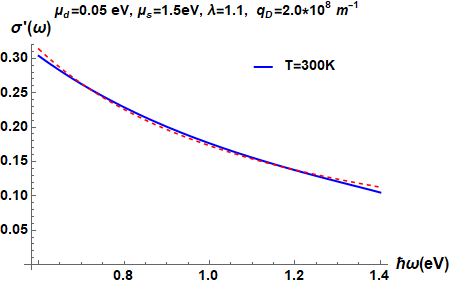
Figure 2 presents the $A.C.$ conductivity behaviour of the Kondo-lattice system. Figure 2 (a) presents the real part of the $A.C.$ conductivity for the values of the fitting parameters $\mu_{d}=0.05eV,\mu_{s}=1.5eV,\lambda=1.1$ and $q_{D}=2.0\times 10^{8}m^{-1}$. In high frequency regime $\frac{1}{\omega}$ fitting for the real part of conductivity is performed using the the least square fitting method. Figure 3 shows least square fitting in high frequency regime (tail part of figure 3). Red dashed line shows $\frac{1}{\omega}$ comparison. Thus, it is found that the tail part of the real conductivity scales to $\frac{1}{\omega}$. In real $\sigma(\omega)$ at lower frequencies we observe the Drude peak and at higher $\omega$ we observe that $\sigma(\omega)\sim\frac{1}{\omega}$ (instead of $\frac{1}{\omega^{2}}$ Drude law) [3, 9]. Figure 3 shows least square fitting in high frequency regime (tail part of figure 3). Red dashed line shows $\frac{1}{\omega}$ comparison.

The calculations of $A.C.$ conductivity using the memory function formalism for the Kondo-lattice Hamiltonian is presented. Using the Wölfle-Götze equation of motion method the frequency dependent memory function is computed. The general memory function is expanded under the long wavelength limit and frequency dependent imaginary part of the memory function is calculated. The numerical computation of the real part of the memory function is performed using the Krammers-Kronig transformation. I found that real part conductivity shows the Drude peak at lower frequency and at higher frequency conductivity deviates from the Drude law and scales as $\frac{1}{\omega}$.

The terms for expression (23) are

	$$\displaystyle h_{1}(\epsilon,\hbar\omega)=\frac{\sqrt{\epsilon-\hbar\omega}}{(1+e^{\beta(\epsilon-\hbar\omega-\mu_{s})})}-\frac{\sqrt{\epsilon+\hbar\omega}}{(1+e^{\beta(\epsilon+\hbar\omega-\mu_{s})})}$$		(25)
	$$\displaystyle h_{2}(\epsilon,\hbar\omega)=\frac{1}{\sqrt{\epsilon-\hbar\omega}(1+e^{\beta(\epsilon-\hbar\omega-\mu_{s})})}-\frac{1}{\sqrt{\epsilon+\hbar\omega}(1+e^{\beta(\epsilon+\hbar\omega-\mu_{s})})}$$		(26)
	$$\displaystyle~{}~{}~{}~{}~{}~{}~{}~{}~{}~{}~{}~{}~{}~{}-2\beta\frac{\sqrt{\epsilon-\hbar\omega}e^{\beta(\epsilon-\hbar\omega-\mu_{s})}}{(1+e^{\beta(\epsilon-\hbar\omega-\mu_{s})})}+2\beta\frac{\sqrt{\epsilon+\hbar\omega}e^{\beta(\epsilon+\hbar\omega-\mu_{s})}}{(1+e^{\beta(\epsilon+\hbar\omega-\mu_{s})})}$$		(27)
	$$\displaystyle h_{3}(\epsilon,\hbar\omega)=\sqrt{\epsilon+\hbar\omega}-\sqrt{\epsilon-\hbar\omega},~{}~{}~{}~{}~{}~{}~{}h_{4}(\epsilon,\hbar\omega)=\frac{1}{\sqrt{\epsilon+\hbar\omega}}-\frac{1}{\sqrt{\epsilon-\hbar\omega}},$$		(28)

and $\Xi$ function are

	$\displaystyle\Xi(\beta\mu_{d})$	$\displaystyle=\int_{-\beta\mu_{d}}^{\infty}\frac{dx\sqrt{x+\beta\mu_{d}}e^{x}}{(e^{x}+1)^{2}}+\frac{2}{3}\int_{-\beta\mu_{d}}^{\infty}\frac{dx(x+\beta\mu_{d})^{\frac{3}{2}}e^{x}}{(e^{x}+1)^{2}}-~{}\frac{4}{3}\int_{-\beta\mu_{d}}^{\infty}\frac{dx(x+\beta\mu_{d})^{\frac{3}{2}}e^{2x}}{(e^{x}+1)^{3}}$		(29)
	$\displaystyle\Xi^{1}(\beta\mu_{d})$	$\displaystyle=\int_{-\beta\mu_{d}}^{\infty}\frac{dx\sqrt{x+\beta\mu_{d}}e^{x}}{(e^{x}+1)^{2}}$		(30)
	$\displaystyle\Xi^{2}(\beta\mu_{d})$	$\displaystyle=\int_{-\beta\mu_{d}}^{\infty}\frac{dx\sqrt{x+\beta\mu_{d}}e^{x}}{(e^{x}+1)^{3}}+\frac{2}{3}\int_{-\beta\mu_{d}}^{\infty}\frac{dx(x+\beta\mu_{d})^{\frac{3}{2}}e^{x}}{(e^{x}+1)^{3}}-\frac{4}{3}\int_{-\beta\mu_{d}}^{\infty}\frac{dx(x+\beta\mu_{d})^{\frac{3}{2}}e^{2x}}{(e^{x}+1)^{4}}.$		(31)

I thank Dr. Navinder Singh for encouragement and important comments.

References

- [1] Neil W Ashcroft, and N David Mermin, and others, Solid state physics, Holt, Rinehart and Winston, New York London, 2005 1976.
- [2] W. Götze and P. Wölfle, Homogeneous dynamical conductivity of simple metals, Physical Review B, 6: 1226–1238, 1972.
- [3] Navinder singh, Electronic transport theories: From weakly to strongly correlated materials, CRC Press, 2017.
- [4] Komal Kumari and Navinder Singh, The memory function formalism: an overview, Eur. J. Phys. 41, 053001, pp 20, 2020.
- [5] Komal Kumari, Raman Sharma and Navinder Singh, J. Phys.:, Condens. Matter, 32, 042603, pp 11, 2020.
- [6] Luxmi Rani and Navinder Singh, Dynamical electrical conductivity of graphene, J. Phys.: Condens. Matter 29, 2555602, 2017.
- [7] Pankaj Bhalla, Nabyendu Das and Navinder Singh,Moment expansion to the memory function for generalized Drude scattering rate, Physics Letters, A 380, 2016.
- [8] Pankaj Bhalla, Pradeep Kumar, Nabyendu Das, and Navinder Singh, Theory of the dynamical thermal conductivity of metals, Phys. Rev. B, 94, pp 115114, 2016.
- [9] Saeed H. Abedinpour, G. Vignale, A. Principi, Marco Polini, Wang-Kong Tse and A. H. MacDonald, Drude weight, plasmon dispersion, and ac conductivity in doped graphene sheets, Phys. Rev. B, American Physical Society 84, 045429, 14, 2011.
- [10] R. Freytag and J. Keller, Dynamical conductivity of heavy fermion systems: effect of impurity scattering, Zeitschrift für Physik B Condensed Matter, 80, 241-247, https://doi.org/10.1007/BF01357509, 1990.
- [11] P. A. Marchetti, G. Orso, Z. B. Su, and L. Yu , In-plane conductivity anisotropy in the underdoped cuprates using the spin-charge gauge approach, American Physical Society, Phys. Rev. B, 69, 21, 214514, 2004.
- [12] Valerio Lucarini, Kai-Erik Peiponen, Jarkko J. Saarinen and Erik M. Vartiainen, Kramers-Kronig relations in optical materials research, Springer Science & Business Media, 110, 2005.
- [13] Christophe Berthod, Jernej Mravlje, Xiaoyu Deng, Rok itko, Dirk van der Marel, and Antoine Georges, Non-Drude universal scaling laws for the optical response of local Fermi liquids, American Physical Society,Phys. Rev. B, 87, 115109, 2013.