Non-Affine Displacements Below Jamming under Athermal Quasi-Static Compression

Considering the process of increasing the density of particle system at zero temperature, if the density is low enough, the particles do not overlap. At a certain density, the particles begin to come into contact, and as a result, the system suddenly gains finite energy, mechanical pressure, and stiffness without any apparent structural changes Van Hecke (2009). This phenomenon called jamming has been actively studied in recent years, and the onset is defined as the jamming transition point $\varphi_{J}$. The jamming transition is ubiquitously observed for very diverse athermal systems such as metallic bolls Bernal and Mason (1960), forms Durian (1995); Katgert and van Hecke (2010), colloids Zhang et al. (2009), polymers Karayiannis et al. (2009), candies Donev et al. (2004), dices Jaoshvili et al. (2010), biological tissues Bi et al. (2015), growing microbes Delarue et al. (2016), and some neural networks Franz and Parisi (2016); Franz et al. (2019).

A famous and popular numerical protocol to generate a jamming configuration is the athermal quasi-static compression (AQC), which combines the affine transformation with successive energy minimization O’Hern et al. (2003). An advantage of this protocol is that one can unambiguously define the jamming transition point $\varphi_{J}$ as the packing fraction $\varphi$ at which the energy after the minimization has a non-zero finite value. With the AQC, extensive work has been done for frictionless, spherical, and purely repulsive particles above jamming $\varphi>\varphi_{J}$. Systematic numerical studies including finite size scaling analyses determine the precise values of the critical exponents in two and three spatial dimensions O’Hern et al. (2003); Goodrich et al. (2012); Charbonneau et al. (2015), and quasi-one dimension Ikeda (2020). The numerical results of the critical exponents well agree with the mean-field predictions in two and three dimensions Wyart et al. (2005); Charbonneau et al. (2014).

Contrarily and somewhat surprisingly, the critical properties of the jamming transition below $\varphi_{J}$ during the AQC have not yet been fully investigated even for frictionless spherical particles. One of the reasons is that the quantities showing the criticality above $\varphi_{J}$, such as the mechanical pressure, energy, and bulk/shear modulus, are trivially zero below $\varphi_{J}$, and other appropriate quantities are not necessarily clear below $\varphi_{J}$ O’Hern et al. (2003). The criticality below $\varphi_{J}$ has been mainly investigated by adding thermal fluctuation Ikeda et al. (2013); Charbonneau et al. (2014), introducing a moving tracer Drocco et al. (2005), considering self-propelled particles Liao and Xu (2018), or quenching from random initial configurations Ikeda et al. (2020); Nishikawa et al. (2020). In particular, extensive work has been conducted on shear-driven systems Marty and Dauchot (2005a); Olsson and Teitel (2007); Hatano (2008); Heussinger and Barrat (2009); Lerner et al. (2012); Kawasaki et al. (2015); Olsson (2019). However, it would be more desirable if one can directly extract the criticality from the configurations during the AQC. A promising study in this direction has been done by Shen et al. Shen et al. (2012). They observed a rapid increase of several physical quantities, such as the displacements of the particle positions, just below $\varphi_{J}$. However, the critical exponent below $\varphi_{J}$ under the AQC has not been calculated yet.

In this work, we characterize the criticality below $\varphi_{J}$ during the AQC by investigating the statistical properties of the non-affine displacements for frictionless spherical particles in three dimensions. We show that the mean square of the non-affine displacements diverges toward $\varphi_{J}$ with the critical exponent very close to that of the shear viscosity. By observing the participation ratio, it is shown that the displacements become more localized as the system approaches $\varphi_{J}$. Furthermore, by using the finite size scaling of the participation ratio, we calculate the fractal dimension of the displacements at $\varphi_{J}$. Finally, we show that the distribution of the non-affine displacements has a power-law tail at $\varphi_{J}$, and prove that there is a scaling relation between the power-law tail and fractal dimension.

We consider $N$ frictionless spherical particles in three dimensions. The interaction potential between $N$ particles is given as

where $\bm{r}_{i}=\{x_{i},y_{i},z_{i}\}$ and $R_{i}$ respectively denote the position and radius of the $i$-th particle. The particles are confined in a cubic box $\bm{r}_{i}\in[0,L]^{3}$ with the periodic boundary conditions in all directions. To avoid crystallization, we use a binary mixture consisting of ${N_{\rm S}=N/2}$ small particles and ${N_{L}=N/2}$ large particles. The radii of large and small particles are $R_{\rm S}=0.5$ and $R_{\rm L}=0.7$, respectively. With those notations, the volume fraction $\varphi$ is written as

The settings of this model are standard ones that have been studied in the context of the jamming transition O’Hern et al. (2003).

Here we describe the AQC originally proposed by O’Hern et al. O’Hern et al. (2003). Starting from a random initial configuration at a small packing fraction, for example $\varphi=0.1$, compression and energy minimization are performed successively in sequence. For each step of the compression, the packing fraction is slightly increased as $\varphi\to\varphi+\varepsilon$ with $\varepsilon=10^{-5}$, by performing the affine transformation $\bm{r}_{i}\to\bm{r}_{i}L(\varphi+\varepsilon)/L(\varphi)$, where $L(\varphi)=\left[2\pi N(R_{\rm S}^{3}+R_{\rm L}^{3})/3\varphi\right]^{1/3}$. Then, the energy is minimized by using the FIRE algorithm, for details see Ref. Bitzek et al. (2006), until the energy or squared force becomes sufficiently small: $V_{N}/N<10^{-16}$ or $\sum_{i=1}^{N}(\nabla_{i}V_{N})^{2}/N<10^{-25}$. The procedure is repeated up to the jamming transition point $\varphi_{J}$ at which $V_{N}/N>10^{-16}$ after the minimization O’Hern et al. (2003).

We perform the numerical simulations for various system sizes $N=256$, $512$, $1024$, $2048$, and $4096$. To improve the statistics, we average over $1000$ samples for $N=256$ and $100$ samples for the other system sizes. We confirmed that the results do not depend on $\varepsilon$, see Appendix A.

When the system is compressed from $\varphi$ to $\varphi+\varepsilon$, the displacement of the $i$-th particle can be written as

where $\delta\bm{r}_{i}^{\rm A}=\left[L(\varphi+\varepsilon)/L(\varphi)-1\right]\bm{r}_{i}(\varphi)$ and $\delta\bm{r}_{i}^{\rm NA}$ respectively denote the affine and non-affine parts of the displacement. In this work, we only focus on the non-trivial part of the displacement $\delta\bm{r}_{i}^{\rm NA}$.

To characterize the criticality of the non-affine displacements, we first observe the mean squared displacement

with

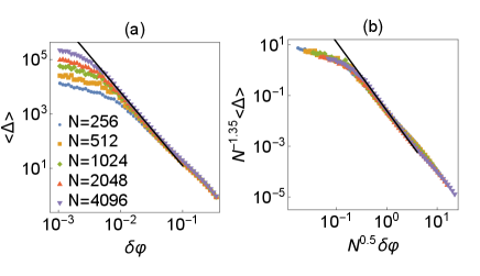
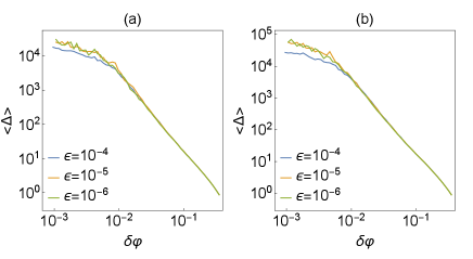
where $\delta l=L(\varphi+\varepsilon)/L(\varphi)-1$ accounts for the change of the linear distance $L$ of the system. In Fig. 1 (a), we show $\left\langle\Delta\right\rangle$ as a function of $\delta\varphi=\varphi_{J}-\varphi$. For large $N$ and intermediate $\delta\varphi$, $\left\langle\Delta\right\rangle$ shows the power law

The power-law fitting of the data for $N=4096$ in the range $\delta\varphi\in(0.01,0.1)$ leads to

see the solid line in Fig. 1 (a). Interestingly, Eq. (7) is close to the theoretical prediction for the critical exponent of the shear viscosity $\beta^{\prime}=2.8$ DeGiuli et al. (2015). We shall discuss a possible connection between $\left\langle\Delta\right\rangle$ and shear viscosity later in this paper.

To further investigate the scaling of $\left\langle\Delta\right\rangle$, we perform a finite-size scaling analysis assuming the following scaling function:

where $\mathcal{D}(x)=O(1)$ for $x\ll 1$, and $\mathcal{D}(x)\sim x^{-\beta}$ for $x\gg 1$. As shown in Fig. 1 (b), a good scaling collapse is obtained with $\alpha=1.35$. This result implies that the number of the correlated particles diverges as $N_{\rm cor}\sim\delta\varphi^{-\beta/\alpha}\sim\delta\varphi^{-2}$, and the correlation length $L_{\rm cor}\sim N_{\rm cor}^{1/3}\sim\delta\varphi^{-\nu}$ with $\nu=2/3\approx 0.67$ under the assumption that the correlated volume is compact. This is close to a previous result $\nu=0.71$ obtained by the finite-size scaling analysis of the transition point O’Hern et al. (2003).

To see the spatial structure of the displacements, we observe the normalized vector Yamamoto and Onuki (1998):

which satisfies $\sum_{i=1}^{N}\bm{e}_{i}\cdot\bm{e}_{i}=1$.

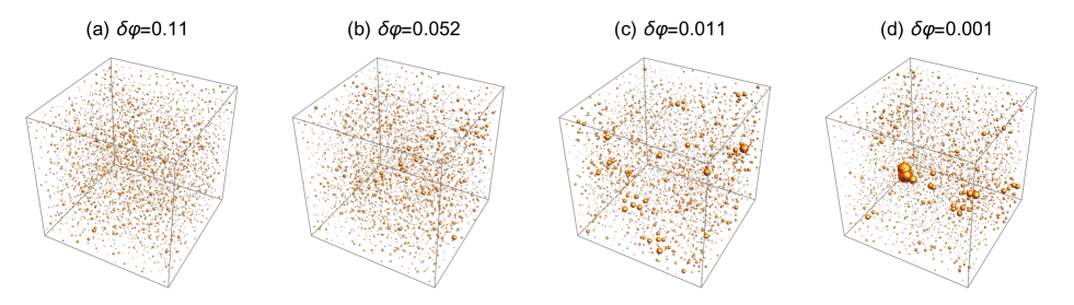
In Fig. 2, we visualize $\bm{e}_{i}$ by drawing spheres such that their radii are proportional to $\left|\bm{e}_{i}\right|$. Far from jamming, the spatial distribution of $\bm{e}_{i}$ is homogeneous and featureless, see Fig. 2 (a). On the contrary, near jamming, a few particles have very large displacements, and thus the displacement is spatially heterogeneous and localized, see Fig. 2 (d).

We quantify the degree of the localization by using the participation ratio:

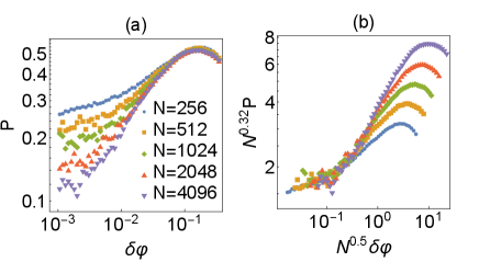
which (or inverse of which) is widely used in the study of condensed matter physics Kramer and MacKinnon (1993), including amorphous solids Lerner et al. (2016); Mizuno et al. (2017). If $\bm{e}_{i}$ is spatially localized to a single particle, say ${\bm{e}_{i}\cdot\bm{e}_{i}=\delta_{i1}}$, the participation ratio $P$ is proportional to $N^{-1}$. On the contrary, if $\bm{e}_{i}$ is extended such that ${\bm{e}_{i}\cdot\bm{e}_{i}\sim N^{-1}}$ for all $i$, $P$ is constant independent of $N$. In Fig. 3 (a), we show the $\delta\varphi$ dependence of $P$. One can see that $P$ decreases with approaching $\varphi_{J}$ and increasing $N$. To investigate the $N$ dependence of $P$, we use the following scaling form:

assuming the same correlated volume as in Eq. (8). We find a good collapse with

near the jamming point, see Fig. 3 (b). At $\varphi_{J}$, $P$ vanishes in the thermodynamic limit as $P\sim N^{-\gamma}$. This exponent relates to the fractal dimension $d_{f}$ of $\bm{e}_{i}$, namely, if $\bm{e}_{i}\cdot\bm{e}_{i}\sim L^{-d_{f}}$ for $i=1,\dots,L^{d_{f}}$, this yields that $P\sim N^{-1+d_{f}/d}$ Kramer and MacKinnon (1993), leading to

Therefore, $\bm{e}_{i}$ has a more compact structure than the bulk $d=3$. A mean-field theory of the jamming transition predicts that the correlated volume $v_{\rm col}$ and correlation length $l_{\rm cor}$ have the following relation $v_{\rm col}\sim l_{\rm cor}^{2}$ Yan et al. (2016); Düring et al. (2016). This may imply that the fractal dimension is $d_{f}=2$, which is close to our estimation Eq. (13).

Interestingly, the similar spatially heterogeneous structures are observed for super-cooled liquids near the glass transition point Ediger (2000). For the studies of the glass transition, the degree of spatial heterogeneity is characterized by the so-called non-gaussian parameter Rahman (1964); Kob and Andersen (1995). In our setting, an analogous quantity may be written as

If the displacements follow the featureless gaussian distribution, one obtains $\alpha_{2}=0$. For the supercooled liquids, $\alpha_{2}$ of the displacements rapidly increases on decreasing the temperature Kob and Andersen (1995); Weeks et al. (2000). Similarly, $\alpha_{2}$ of our model increases on approaching $\varphi_{J}$, because $P\to 0$ and $\alpha_{2}\propto P^{-1}$. Furthermore, an experimental study for the supercooled colloidal suspensions, which approximately behave as hard spheres Pusey and Van Megen (1986); van Megen and Underwood (1994) and may have the same interaction as our model below jamming, showed that the dynamically correlated regions form a compact cluster of the fractal dimension $d_{f}=1.9\pm 0.4$ Weeks et al. (2000), reasonably close to our result of Eq. (13). Also, the inhomogeneous mode-coupling theory, which is a mean-field theory of the glass transition, predicts $d_{f}=2$ in the early stage of the relaxation process Biroli et al. (2006). Those results suggest the existence of the underlying universality between the dynamics of the athermal system near $\varphi_{J}$ and thermal systems near the glass transition point Marty and Dauchot (2005b); Chaudhuri et al. (2007).

Here, we discuss the behavior of $P$ from the perspective of the distribution of $\Delta$. First, we note that $P$ can be written as

where the distribution $f(\Delta)$ of $\Delta$ is defined as

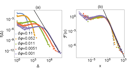
Fig. 4 (a) presents $f(\Delta)$ for several $\delta\varphi$. $f(\Delta)$ has a broader distribution for smaller $\delta\varphi$. For the later convenience, we define a scaled variable $x=\Delta/\left\langle\Delta\right\rangle$, and distribution function

By definition, $\int dx\mathcal{F}(x)=\int dx\mathcal{F}(x)x=1$. As shown in Fig. 4 (b), with decreasing $\delta\varphi$, $\mathcal{F}(x)$ develops the power-law tail

A similar fat-tail was previously reported for the velocity distribution of sheared driven systems in the quasi-static limit near $\varphi_{J}$ Tighe et al. (2010); Andreotti et al. (2012); Olsson (2016). Now, we show that the exponent $\zeta$ relates to $\gamma$ in Eq. (11). Using Eq. (15) and (17), we get

If $\zeta<3$, the denominator diverges, leading to $P=0$ at $\varphi_{J}$. For finite $N$, however, the divergence does not occur as the power law of $\mathcal{F}(x)$ is truncated at finite $x_{\rm max}$. Using the extreme value statistics, we can calculate $x_{\rm max}$ as

Then, $P$ for finite $N$ is expressed as

Comparing this with Eq. (11) for $\delta\varphi=0$, we finally get

This is consistent with the assumption $\zeta<3$ and well agrees with the numerical result, see Fig. 4.

In summary, we investigated the statistical properties of the non-affine displacements under the AQC below the jamming transition point. We showed that the mean square of the non-affine displacement diverges toward the jamming transition point. At the jamming transition point, the distribution of the non-affine displacements has a power-law tail, the exponent of which relates to the fractal dimension.

An interesting question is how the present work relates to the previous works for the shear driven systems. As the shear viscosity $\eta$ diverges with the same critical exponent as the bulk viscosity $\eta_{p}$ near $\varphi_{J}$, namely, $\eta\sim\eta_{p}\sim\delta\varphi^{-\beta^{\prime}}$ Olsson and Teitel (2012); Vågberg et al. (2014), we consider a system compressed with a finite compression rate $\dot{l}=\dot{L}/L$, instead of the shear driven system. The work done by the imposed compression per time is $p\dot{l}L^{3}=\eta_{p}\dot{l}^{2}L^{3}$, where $p$ denotes the pressure, and $\eta_{p}=p/\dot{l}$ denotes the bulk viscosity. In the quasi-static limit $\dot{l}\to 0$, this should be balanced with the dissipation $\sum_{i=1}^{N}\left(\dot{\bm{r}}_{i}^{\rm NA}\right)^{2}$, leading to Lerner et al. (2012); Katgert et al. (2013)

A mean-field theory of sheared suspensions predicts $\eta\sim\delta\varphi^{-\beta^{\prime}}$ with $\beta^{\prime}=2.8$ DeGiuli et al. (2015), which is close to our result ${\left\langle\Delta\right\rangle\sim\delta\varphi^{-\beta}}$ with $\beta=2.7$ and thus supports the above conjecture. However, the numerical result of $\beta^{\prime}$ varies widely from one literature to another. For instance, Ref. Kawasaki et al. (2015) reported $\beta^{\prime}=2.55$, while Ref. Olsson (2019) reported $\beta^{\prime}=3.82$. Further study is necessary to elucidate this point.

From a practical point of view, the AQC has several advantages over other dynamical methods such as implying shear to characterize the criticality below jamming. First of all, our method is much efficient, as we do not need to wait that the system reaches the steady state. Furthermore, the method allows us to reduce the fitting parameters because the jamming transition point $\varphi_{J}$ is determined during the procedure. Therefore, we believe that the AQC facilitates the investigation of the criticality below jamming for frictionless spherical particles, and hopefully for other models such as non-spherical particles and frictional particles. For frictional particles, it is reported that the waiting time and its distribution show the power-law behaviors near the (shear) jamming transition point Pastore et al. (2011); Srivastava et al. (2019). It is an interesting future work to see if such critical behaviors of the dynamical quantities appear under the AQC protocol.

The mean-field theory predicts that the correlated volume has the fractal dimension $d_{f}=2$, irrespective of the spatial dimension $d$ Yan et al. (2016); Düring et al. (2016). If this is the case, the similar argument above Eq. (13) leads to

and that of Eq. (22) leads to

We obtained numerical results consistent with Eqs. (24) and (25) in three dimension $d=3$. It is tempting to test if Eqs. (24) and (25) hold in other $d$. In particular, $\gamma=0$ in $d=2$, suggesting that the participation ratio $P$ at $\varphi_{J}$ may exhibit the logarithmic dependence on $N$, instead of a power law. This deserves further study.

References

- Van Hecke (2009) M. Van Hecke, J. Phys. Condens. Matter 22, 033101 (2009).
- Bernal and Mason (1960) J. Bernal and J. Mason, Nature 188, 910 (1960).
- Durian (1995) D. J. Durian, Phys. Rev. Lett. 75, 4780 (1995).
- Katgert and van Hecke (2010) G. Katgert and M. van Hecke, EPL 92, 34002 (2010).
- Zhang et al. (2009) Z. Zhang, N. Xu, D. T. Chen, P. Yunker, A. M. Alsayed, K. B. Aptowicz, P. Habdas, A. J. Liu, S. R. Nagel, and A. G. Yodh, Nature 459, 230 (2009).
- Karayiannis et al. (2009) N. C. Karayiannis, K. Foteinopoulou, and M. Laso, J. Chem. Phys. 130, 164908 (2009).
- Donev et al. (2004) A. Donev, I. Cisse, D. Sachs, E. A. Variano, F. H. Stillinger, R. Connelly, S. Torquato, and P. M. Chaikin, Science 303, 990 (2004).
- Jaoshvili et al. (2010) A. Jaoshvili, A. Esakia, M. Porrati, and P. M. Chaikin, Phys. Rev. Lett. 104, 185501 (2010).
- Bi et al. (2015) D. Bi, J. Lopez, J. Schwarz, and M. L. Manning, Nat. Phys. 11, 1074 (2015).
- Delarue et al. (2016) M. Delarue, J. Hartung, C. Schreck, P. Gniewek, L. Hu, S. Herminghaus, and O. Hallatschek, Nat. Phys. 12, 762 (2016).
- Franz and Parisi (2016) S. Franz and G. Parisi, J. Phys. A 49, 145001 (2016).
- Franz et al. (2019) S. Franz, S. Hwang, and P. Urbani, Phys. Rev. Lett. 123, 160602 (2019).
- O’Hern et al. (2003) C. S. O’Hern, L. E. Silbert, A. J. Liu, and S. R. Nagel, Phys. Rev. E 68, 011306 (2003).
- Goodrich et al. (2012) C. P. Goodrich, A. J. Liu, and S. R. Nagel, Phys. Rev. Lett. 109, 095704 (2012).
- Charbonneau et al. (2015) P. Charbonneau, E. I. Corwin, G. Parisi, and F. Zamponi, Phys. Rev. Lett. 114, 125504 (2015).
- Ikeda (2020) H. Ikeda, Phys. Rev. Lett. 125, 038001 (2020).
- Wyart et al. (2005) M. Wyart, L. E. Silbert, S. R. Nagel, and T. A. Witten, Phys. Rev. E 72, 051306 (2005).
- Charbonneau et al. (2014) P. Charbonneau, J. Kurchan, G. Parisi, P. Urbani, and F. Zamponi, Nat. Commun. 5, 1 (2014).
- Ikeda et al. (2013) A. Ikeda, L. Berthier, and G. Biroli, J. Chem. Phys. 138, 12A507 (2013).
- Drocco et al. (2005) J. A. Drocco, M. B. Hastings, C. J. O. Reichhardt, and C. Reichhardt, Phys. Rev. Lett. 95, 088001 (2005).
- Liao and Xu (2018) Q. Liao and N. Xu, Soft Matter 14, 853 (2018).
- Ikeda et al. (2020) A. Ikeda, T. Kawasaki, L. Berthier, K. Saitoh, and T. Hatano, Phys. Rev. Lett. 124, 058001 (2020).
- Nishikawa et al. (2020) Y. Nishikawa, A. Ikeda, and L. Berthier, arXiv preprint arXiv:2007.09418 (2020).
- Marty and Dauchot (2005a) G. Marty and O. Dauchot, Phys. Rev. Lett. 94, 015701 (2005a).
- Olsson and Teitel (2007) P. Olsson and S. Teitel, Phys. Rev. Lett. 99, 178001 (2007).
- Hatano (2008) T. Hatano, J. Phys. Soc. Jpn. 77, 123002 (2008).
- Heussinger and Barrat (2009) C. Heussinger and J.-L. Barrat, Phys. Rev. Lett. 102, 218303 (2009).
- Lerner et al. (2012) E. Lerner, G. Düring, and M. Wyart, PNAS 109, 4798 (2012).
- Kawasaki et al. (2015) T. Kawasaki, D. Coslovich, A. Ikeda, and L. Berthier, Phys. Rev. E 91, 012203 (2015).
- Olsson (2019) P. Olsson, Phys. Rev. Lett. 122, 108003 (2019).
- Shen et al. (2012) T. Shen, C. S. O’Hern, and M. D. Shattuck, Phys. Rev. E 85, 011308 (2012).
- Bitzek et al. (2006) E. Bitzek, P. Koskinen, F. Gähler, M. Moseler, and P. Gumbsch, Phys. Rev. Lett. 97, 170201 (2006).
- DeGiuli et al. (2015) E. DeGiuli, G. Düring, E. Lerner, and M. Wyart, Phys. Rev. E 91, 062206 (2015).
- Yamamoto and Onuki (1998) R. Yamamoto and A. Onuki, Phys. Rev. Lett. 81, 4915 (1998).
- Kramer and MacKinnon (1993) B. Kramer and A. MacKinnon, Rep. Prog. Phys. 56, 1469 (1993).
- Lerner et al. (2016) E. Lerner, G. Düring, and E. Bouchbinder, Phys. Rev. Lett. 117, 035501 (2016).
- Mizuno et al. (2017) H. Mizuno, H. Shiba, and A. Ikeda, PNAS 114, E9767 (2017).
- Yan et al. (2016) L. Yan, E. DeGiuli, and M. Wyart, EPL 114, 26003 (2016).
- Düring et al. (2016) G. Düring, E. Lerner, and M. Wyart, Phys. Rev. E 94, 022601 (2016).
- Ediger (2000) M. D. Ediger, Annu. Rev. Phys. Chem. 51, 99 (2000).
- Rahman (1964) A. Rahman, Phys. Rev. 136, A405 (1964).
- Kob and Andersen (1995) W. Kob and H. C. Andersen, Phys. Rev. E 51, 4626 (1995).
- Weeks et al. (2000) E. R. Weeks, J. C. Crocker, A. C. Levitt, A. Schofield, and D. A. Weitz, Science 287, 627 (2000).
- Pusey and Van Megen (1986) P. N. Pusey and W. Van Megen, Nature 320, 340 (1986).
- van Megen and Underwood (1994) W. van Megen and S. M. Underwood, Phys. Rev. E 49, 4206 (1994).
- Biroli et al. (2006) G. Biroli, J.-P. Bouchaud, K. Miyazaki, and D. R. Reichman, Phys. Rev. Lett. 97, 195701 (2006).
- Marty and Dauchot (2005b) G. Marty and O. Dauchot, Phys. Rev. Lett. 94, 015701 (2005b).
- Chaudhuri et al. (2007) P. Chaudhuri, L. Berthier, and W. Kob, Phys. Rev. Lett. 99, 060604 (2007).
- Tighe et al. (2010) B. P. Tighe, E. Woldhuis, J. J. C. Remmers, W. van Saarloos, and M. van Hecke, Phys. Rev. Lett. 105, 088303 (2010).
- Andreotti et al. (2012) B. Andreotti, J.-L. Barrat, and C. Heussinger, Phys. Rev. Lett. 109, 105901 (2012).
- Olsson (2016) P. Olsson, Phys. Rev. E 93, 042614 (2016).
- Olsson and Teitel (2012) P. Olsson and S. Teitel, Phys. Rev. Lett. 109, 108001 (2012).
- Vågberg et al. (2014) D. Vågberg, P. Olsson, and S. Teitel, Phys. Rev. Lett. 113, 148002 (2014).
- Katgert et al. (2013) G. Katgert, B. P. Tighe, and M. van Hecke, Soft Matter 9, 9739 (2013).
- Pastore et al. (2011) R. Pastore, M. P. Ciamarra, and A. Coniglio, Philosophical Magazine 91, 2006 (2011).
- Srivastava et al. (2019) I. Srivastava, L. E. Silbert, G. S. Grest, and J. B. Lechman, Phys. Rev. Lett. 122, 048003 (2019).
- Vågberg et al. (2011) D. Vågberg, P. Olsson, and S. Teitel, Phys. Rev. E 83, 031307 (2011).