NOMA-Based Coexistence of Near-Field and Far-Field Massive MIMO Communications
Abstract
This letter considers a legacy massive multiple-input multiple-output (MIMO) network, in which spatial beams have been preconfigured for near-field users, and proposes to use the non-orthogonal multiple access (NOMA) principle to serve additional far-field users by exploiting the spatial beams preconfigured for the legacy near-field users. Our results reveal that the coexistence between near-field and far-field communications can be effectively supported via NOMA, and that the performance of NOMA-assisted massive MIMO can be efficiently improved by increasing the number of antennas at the base station.
Index Terms:
Non-orthogonal multiple access (NOMA), near-field communications, beamforming.I Introduction
One recent advance in non-orthogonal multiple access (NOMA) is its use as an add-on in a massive multiple-input multiple-output (MIMO) based legacy space division multiple access (SDMA) network, where spatial beams preconfigured for legacy users are used to serve additional users [1]. As a result, the connectivity and the overall system throughput of SDMA can be improved in a low-complexity and spectrally efficient manner. For conventional SDMA networks based on far-field communications, where the transceiver distance is larger than the Rayleigh distance [2], this application of NOMA is intuitive, as explained in the following. Far-field beamforming is based on steering vectors, i.e., the spatial beams are cone-shaped [3]. In practice, each of these cone-shaped beams can cover a large area, and it is intuitive to encourage multiple users which are inside of one cone-shaped area to exploit the same beam via NOMA.
Near-field communications have received a lot of attention as, for high carrier frequencies and large numbers of antennas, the Rayleigh distance becomes significantly large [4, 5]. Unlike far-field communications, the spherical-wave channel model has to be used for near-field communications, which motivates the use of beam-focusing, i.e., a beam is focused on not only a spatial direction but also a specific location [6]. As a result, a naturally arising question is whether the preconfigured spatial beams in near-field communication networks can still be used to admit additional users in the same manner as far-field beams, which is the motivation for this work.
This letter considers a legacy near-field SDMA network, in which spatial beams have been preconfigured for legacy near-field users, and proposes to apply the principle of NOMA to serve additional far-field users by exploiting these preconfigured spatial beams. A resource allocation optimization problem is formulated to maximize the far-field users’ sum data rate while guaranteeing the legacy near-field users’ quality-of-service (QoS) requirements. First, a suboptimal low-complexity algorithm based on successive convex approximation (SCA) is proposed to solve the problem, and then the optimal performance is obtained for two special cases by applying the branch-and-bound (BB) algorithm [7, 8]. Simulation results are presented to demonstrate that the use of NOMA can effectively support the coexistence of near-field and far-field communications, and the performance of NOMA assisted massive MIMO can be efficiently improved by increasing the number of antennas at the base station.
II System Model
Consider a legacy downlink near-field SDMA network, in which a base station employs an -antenna uniform linear array (ULA) and serves single-antenna near-field users, where . In this letter, it is assumed that near-field beamforming vectors, denoted by , have already been configured to serve the legacy users individually. The aim of this letter is to admit additional far-field users based on these preconfigured spatial beams. Denote the -dimensional coordinates of the -th near-field user, the -th far-field user, the center of the array, and the -th element of the array by , , , and , respectively. According to the principle of near-field communications, , and , where , , and denote the Rayleigh distance, the wavelength, and the antenna spacing of the ULA, respectively [6, 9, 10]. We note that other types of antenna arrays, such as uniform planar arrays (UPAs) and uniform circular arrays (UCAs), can also be used for supporting near-field communications [4, 11].
II-A Near-Field and Far-Field Channel Models
The -th legacy near-field user’s observation is given by , where denotes the signal vector sent by the base station, denotes the additive Gaussian noise with its power denoted by , is based on the spherical-wave propagation model [5, 6, 12]:
| (1) |
where , , and denote the free-space path loss, the speed of light, and the carrier frequency, respectively. We note that the line of sight (LoS) path is assumed to be available for the near-field users, as they are within the Rayleigh distance from the base station [6, 12].
The -th far-field user receives the following signal: , where denotes the additive Gaussian noise having the same power as , the conventional beamsteering vector is used to model the far-field user’s channel vector, , as follows: [2]
| (2) |
and denotes the conventional angle of departure. Scheduling is assumed to be carried out to ensure that each participating far-field user has an LoS connection to the base station. Because the LoS link is typically dB stronger than the non-LoS links, only the LoS link is considered in (1) and (2) [13].
Remark 1: Comparing (1) to (2), one can observe that the near-field channel model is fundamentally different from the far-field one. In particular, the channel vector in (2) is mainly parameterized by the angle of departure, , but the elements of the vector in (1) depend on the near-field user’s specific location.
II-B Near-Field Beamforming and NOMA Data Rates
For illustrative purposes, full-digital near-field beamforming based on the zero-forcing principle is adopted in this letter: , where , and is an diagonal matrix to ensure power normalization. In particular, the -th element on the main diagonal of is given by , which ensures that the beamforming vectors are normalized, i.e., , for all .
The NOMA principle is applied to ensure that each preconfigured spatial beam is used as a type of bandwidth resource for serving additional far-field users, which means that the signal vector sent by the base station is given by
| (3) |
where is the transmit power allocated to the -th near-field user’s signal, denotes the coefficient assigned to the -th far-field user on beam , and and denote the signals for the near-field and far-field users, respectively. If the -th far-field user uses only a single beam, can be viewed as a power allocation coefficient. If multiple beams are used, can be interpreted as a beamforming coefficient.
Therefore, the observation at the -th near-field user can be written as follows:
| (4) |
For the considered NOMA network, the near-field users have better channel conditions than the far-field users, and hence have the capability to carry out SIC. To reduce the system complexity, assume that at most a single far-field user is scheduled on a near-field user’s beam, and each of the far-field users utilize beams, where . Denote the subset collecting the indices of the beams used by the -th far-field user by , where .
Assume that the -th far-field user is active on . On the one hand, this far-field user’s signal can be decoded by the -th near-field user with the following data rate: , where . If the first stage of SIC is successful, the near-field user can remove the far-field user’s signal and decode its own signal with the following data rate: .
On the other hand, the -th far-field user directly decodes its own signal with the following data rate:
where , , and .
The aim of this letter is to maximize the far-field users’ sum data rate while guaranteeing the near-field users’ QoS requirements, based on the following optimization problem:
| (P1a) | ||||
| (P1b) | ||||
| (P1c) | ||||
| (P1d) | ||||
where denotes an indicator function, i.e., if , otherwise , denotes the near-field users’ target data rate, and denotes the transmit budget per beam. We note that the resource allocation problem in (P1) requires the base station to have access to the users’ channel state information (CSI). This CSI assumption can be realized by asking each user to first carry out channel estimation based on the pilots broadcast by the base station and then feed back its CSI to the base station via a reliable control channel.
Remark 2: The objective function in (P1a) indicates that the -th far-field user prefers to use a beam on which both and are strong. Therefore, to find and remove the indicator function in (P1a), a simple sub-optimal scheduling scheme can be used first, where the far-field users are successively asked to select the best beams based on the following criterion: . Here, the channel gains, and , are normalized to ensure that they are in the same order of magnitude. As a result, for , and only , , need to be optimized. We note that optimal scheduling is possible by applying integer programming as in [8]. However, this is out of the scope of this paper due to the space limitations.
III Proposed Resource Allocation Algorithms
III-A SCA-based Resource Allocation
In this section, the general case with and is considered first. Problem (P1) can be first recast as follows:
| (P2a) | ||||
| (P2b) | ||||
| (P2c) | ||||
| (P2d) | ||||
| (P2e) | ||||
| (P2f) | ||||
where , and constraint (P2d) is due to the use of the scheduling scheme discussed in Remark 3. Because (P2b) and (P2c) are decreasing functions of , it is straightforward to show that the optimal solution of is . We note that the main challenges involving problem (P2) are the non-convex constraints in (P2b) and (P2c), which motivates the use of SCA. To facilitate the application of SCA, problem (P2) can be first recast as follows:
| (P3a) | ||||
| (P3b) | ||||
| (P3c) | ||||
| (P3d) | ||||
where and . The term can be approximated as an affine function via the Taylor expansion. In particular, first express as follows:
| (5) |
where denote the transpose, , , . By building the real-valued vector, , and applying the first order Taylor expansion, can be approximated as follows:
| (6) |
where denotes the initial value of , and is given by
| (7) |
Constraint (P3c) can be similarly approximated by using an initial value .
Therefore, problem (P3) can be approximated as follows:
| (P4a) | ||||
| (P4b) | ||||
| (P4c) | ||||
which is a convex optimization problem and can be straightforwardly solved by convex solvers.
The implementation of SCA requires that is a feasible solution of problem (P3), and can be obtained as follows. First, by using (P3d), we choose for , and for , which means that the following choices of , , are feasible:
| (8) |
Based on , SCA can be applied in an iterative manner, i.e., by using and solving problem (P4), a new estimate of can be generated and used to replace in the next iteration. In general, SCA can only converge to a stationary point, which cannot be guaranteed to be the optimal solution. Motivated by this, the optimal performance of NOMA transmission is studied for the two special cases in the following subsection.
III-B Optimal Performance in Two Special Cases
III-B1 Special case with
If there is a single far-field user, i.e., , problem (P1) can be simplified as follows:111The subscript, , is omitted since there is a single far-field user.
| (P5a) | ||||
| (P5b) | ||||
| (P5c) | ||||
| (P5d) | ||||
By following steps similar to those in the previous subsection, problem (P5) can be recast as follows:
| (P6a) | ||||
| (P6b) | ||||
| (P6c) | ||||
| (P6d) | ||||
where , , , and . While problem (P6) is not convex, it can be solved by using the following lemma.
1.
The optimal value of problem (P6) is the same as that of the following optimization problem:
| (P7a) | ||||
| (P7b) | ||||
where .
Proof.
Denote a feasible solution of problem (P6) by . Constraint (P6b) ensures that . Because , , which means that any feasible solution of problem (P6) is also feasible for problem (P7). In other words, the feasible set of problem (P6) is a subset of that of problem (P7), and hence the optimal value of problem (P7) is no less than that of problem of (P6). We also note that the optimal solution of problem (P7) leads to a feasible solution of problem (P6). For example, assume that is the optimal solution of problem (P7). must be feasible to problem (P6), where is the argument of the complex-valued number . By using the fact that the optimal value of problem (P7) is no less than that of problem of (P6), must be the optimal value of problem (P6) as well. Therefore, problems (P6) and (P7) have the same optimal value, and the proof is complete. ∎
By using Lemma 1, the optimal performance of NOMA transmission in the special case with can be obtained by defining and transferring problem (P7) into the following equivalent convex form:
| (P8a) | ||||
III-B2 Special case with
If each far-field user uses a single beam, problem (P1) can be simplified as follows:
| (P9a) | ||||
| (P9b) | ||||
| (P9c) | ||||
| (P9d) | ||||
where denotes the index of the beam used by the -th far-field user, and is simplified to for this special case.

For this special case, problem (P9) is similar to conventional power allocation in interference channels, where the BB algorithm can be used to obtain the optimal solution [7, 8]. Due to the space limitations, the principle of the BB algorithm is described only briefly in the following. As shown in Algorithm 1, the initilization of the algorithm builds an initial box, denoted by , by using an upper bound on as follows: .
In each iteration of the BB algorithm, the key step is to calculate the upper and lower bounds for a box, , which are denoted by and , respectively. Further denote the minimum and maximum vertices of by and , respectively. and , if is a solution of the following feasibility optimization problem:
| (P10a) | ||||
| (P10b) | ||||
| (P10c) | ||||
| (P10d) | ||||
where and are the -th elements of and , respectively. If is not feasible, the upper and lower bounds are set as . The details for implementing the BB algorithm can be found in [8].
IV Simulation Results
In this section, simulation results are presented to evaluate the performance of the proposed NOMA scheme. For all simulations we used, GHz, , bits per channel use, dBm, and [6]. The ULA is placed on the vertical coordinate axis and .
In Fig. 1, the performance of NOMA transmission is evaluated with randomly located users. In particular, the near-field users are uniformly located inside of a half-ring with its inner and outer radii being m and m, respectively. The far-field users are uniformly located inside of a half-ring with its inner and outer radii being m and m, respectively. A greedy resource allocation scheme based on (8) is used as a benchmarking scheme in the figure. As can be seen from Fig. 1, the use of NOMA ensures that the spatial beams preconfigured for the near-field users are efficiently utilized to support additional far-field users. Comparing Fig. 1(a) to Fig. 1(b), one can also observe that the use of more antennas at the base station can further improve the performance of NOMA, which indicates the importance of NOMA for massive MIMO.

In Fig. 2, the impact of imperfect CSI on NOMA is studied. We assume that the perfect CSI of the legacy near-field users is available at the base station, but there exist CSI errors for the far-field users. The estimated CSI is modelled as , where denotes the CSI errors due to imperfect CSI feedback or abrupt changes in the users’ channels, denotes a parameter to measure the quality of the CSI, and follows a complex Gaussian distribution with zero mean and variance [14]. Fig. 2 shows that the performance of NOMA is degraded by imperfect CSI, particularly for large . Fig. 2 also shows that the proposed SCA scheme still outperforms the baseline, even in the presence of imperfect CSI. We note that robust beamforming can be used to combat the detrimental effects of imperfect CSI, which is beyond the scope of this paper.
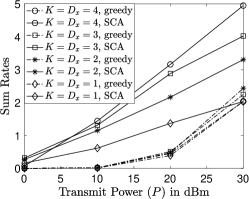
As shown in Sections III-B1 and III-B2, the optimal performance of NOMA transmission can be obtained for the two special cases, which are studied in Fig. 3 by focusing the following deterministic case. On the one hand, assume that the near-field users are equally spaced with m distance, and located within a square with its center located at m. On the other hand, assume that the far-field users are also equally spaced and located on a half-circle with radius meters. Fig. 3(a) focuses on the scenario with a single scheduled far-field user, and Fig. 3(b) focuses on the scenario with a single available beam. Fig. 3 shows that the far-field user’s performance can be improved by using more beams, and there is an optimal choice of for sum-rate maximization. Fig. 3 also shows that SCA provides a reasonable estimate for the optimal performance.


V Conclusions
This letter has considered a legacy network, where spatial beams have been preconfigured for legacy near-field users, and shown that via NOMA, additional far-field users can be efficiently served by using these preconfigured beams. In this letter, each user was assumed to have a single antenna. An important direction for future research is to study the design of NOMA assisted transmission for users equipped with multiple antennas. Furthermore, perfect SIC has been assumed. The study of the impact of imperfect SIC on NOMA constitutes another important direction for future research.
References
- [1] Z. Ding, “NOMA beamforming in SDMA networks: Riding on existing beams or forming new ones?” IEEE Commun. Lett., vol. 26, no. 4, pp. 868–871, Apr. 2022.
- [2] R. W. Heath, N. Gonzalez-Prelcic, S. Rangan, W. Roh, and A. M. Sayeed, “An overview of signal processing techniques for millimeter wave MIMO systems,” IEEE J. Sel. Topics Signal Process., vol. 10, no. 3, pp. 436–453, Apr. 2016.
- [3] Y. Zou, W. Rave, and G. Fettweis, “Analog beamsteering for flexible hybrid beamforming design in mmWave communications,” in Proc. EuCNC, Athens, Greece, Jun. 2016.
- [4] E. Björnson and L. Sanguinetti, “Power scaling laws and near-field behaviors of massive MIMO and intelligent reflecting surfaces,” IEEE O. J. of the Commun. Society, vol. 1, pp. 1306–1324, 2020.
- [5] J. Zhu, Z. Wan, L. Dai, M. Debbah, and H. V. Poor, “Electromagnetic information theory: Fundamentals, modeling, applications, and open problems,” Available on-line at arXiv:2209.09562, 2022.
- [6] H. Zhang et al., “Beam focusing for near-field multiuser MIMO communications,” IEEE Trans. Wireless Commun., vol. 21, no. 9, pp. 7476–7490, Sept. 2022.
- [7] P. C. Weeraddana, M. Codreanu, M. Latva-aho, and A. Ephremides, “Weighted sum-rate maximization for a set of interfering links via branch and bound,” IEEE Trans. Signal Process., vol. 59, no. 8, pp. 3977–3996, Aug. 2011.
- [8] Z. Ding and H. V. Poor, “Joint beam management and power allocation in THz-NOMA Networks,” IEEE Trans. Commun., to appear in 2023.
- [9] K. Chen, C. Qi, and C.-X. Wang, “Two-stage hybrid-field beam training for ultra-massive MIMO systems,” in Proc. 2022 IEEE/CIC Int. Conf. on Commun. in China (ICCC), Foshan, China, Sept. 2022.
- [10] D. Acharya, J. Kokkoniemi, A. Parssinen, and M. Berg, “Performance comparison of near-field focused and conventional phased antenna arrays at 140 GHz,” in Proc. EuCNC, Porto, Portugal, Jun. 2021, pp. 1–6.
- [11] Z. Wu, M. Cui, and L. Dai, “Enabling more users to benefit from near-field communications: From linear to circular array,” Available on-line at arXiv:2212.14654, 2022.
- [12] X. Zhang, H. Zhang, and Y. C. Eldar, “Near-field sparse channel representation and estimation in 6G wireless communications,” Available on-line at arXiv:2212.13527, 2022.
- [13] G. Lee, Y. Sung, and J. Seo, “Randomly-directional beamforming in millimeter-wave multiuser MISO downlink,” IEEE Trans. Wirel. Commun., vol. 15, no. 2, pp. 1086–1100, Feb. 2016.
- [14] Z. Ding, “Robust beamforming design for OTFS-NOMA,” IEEE O. J. Commun. Society, vol. 1, pp. 33–40, 2020.