Noisy Speech Based Temporal Decomposition to Improve Fundamental Frequency Estimation
Abstract
This paper introduces a novel method to separate noisy speech into low or high frequency frames, in order to improve fundamental frequency (F0) estimation accuracy. In this proposal, the target signal is analyzed by means of the ensemble empirical mode decomposition. Next, the pitch information is extracted from the first decomposition modes. This feature indicates the frequency region where the F0 of speech should be located, thus separating the frames into low-frequency (LF) or high-frequency (HF). The separation is applied to correct candidates extracted from a conventional fundamental frequency detection method, and hence improving the accuracy of F0 estimate. The proposed method is evaluated in experiments with CSTR and TIMIT databases, considering six acoustic noises under various signal-to-noise ratios. A pitch enhancement algorithm is adopted as baseline in the evaluation analysis considering three conventional estimators. Results show that the proposed method outperforms the competing strategies, in terms of low/high frequency separation accuracy. Moreover, the performance metrics of the F0 estimation techniques show that the novel solution is able to better improve F0 detection accuracy when compared to competitive approaches under different noisy conditions.
Index Terms:
TF decomposition, Low/High frequency separation, F0 estimation, noisy speech.I Introduction
Urban noisy acoustic scenarios may affect speech temporal and spectral attributes. A robust estimation of the fundamental frequency (F0) feature is a requirement for a diversity applications, such as speech coding [1], speech synthesis [2], speaker and speech [3], [4] recognition. In a voiced speech segment, the F0 consists on the vibration rate of the vocal folds, which corresponds to the inverse of the pitch period. The investigation of harmonic noisy components of speech signals has also gained significant attraction for strategies that attain intelligibility gain [5], [6], [7]. These harmonic components and also the formants play a significant role for speech intelligibility in noise [8], [9], [10]. Therefore, methods and systems which estimate fundamental frequency accurately need to be explored, particularly, at low signal-to-noise ratios (SNRs), where noise components may cause errors in estimation algorithms.
Several approaches have been proposed in the literature for F0 detection in the clean speech. Classical time domain methods are generally based on the Auto-Correlation Function (ACF) [11], [12]. YIN [13] is an alternative solution that uses the local minima of the Normalized Mean Difference Function (NMDF) with some post-processing procedures to avoid estimation errors caused by signal amplitude changes. Nevertheless, SHR [14] and SWIPE [15] are examples of spectral techniques. The SHR method introduces the concept of sub-harmonic to harmonic ratio, and F0 detection is performed by looking for values which maximize this ratio. SWIPE estimates the F0 as the frequency of the sawtooth waveform whose spectrum best matches the spectrum of the input signal. Despite the variety of proposed methods, an accurate estimation of F0 in severe noisy conditions is still a challenging task in speech signal processing.
In recent years, solutions have been proposed for F0 estimation in noisy speech [16], [17], [18]. In [16], the Pitch Estimation Filter with Amplitude Compression (PEFAC) is introduced, which applies a prefiltering to reduce the noise effects with interesting accuracy results. Machine learning based approaches [19], [20], [21], [22] investigate classifiers that include feed-forward, recurrent and convolutional neural networks. Furthermore, other F0 detection methods [23] [24] are based on the Hilbert-Huang Transform (HHT) [25]. Specifically, the Empirical Mode Decomposition (EMD) [25] or its variations, which realizes a time-frequency (TF) decomposition to analyze the noisy speech signal for various tasks [26], [27], [28]. In the HHT-Amp technique [24] the F0 estimates are achieved from the instantaneous amplitude functions of the target signal. Although these F0 estimation methods are examined for noisy environments, some errors can still occur, e.g., F0 subharmonics detection, octave errors, and indistinct periodic background noise from the voiced speech [29].
In a recent work [30], a strategy is introduced to improve pitch detection attained by conventional estimation algorithms considering noisy scenarios. To this end, a Deep Convolutional Neural Network (DCNN) is trained in order to classify the voiced speech frames into low or high frequency. According to the classification, new F0 candidates are computed considering typical probable types of errors for a certain F0 value estimated by a detection method. Taking into account a procedure which involves two spectral attributes of speech frames and a cost function, the enhanced pitch is selected from the new candidates.

This work introduces a method (PRO) to separate harmonic noisy speech into low-frequency or high-frequency frames, in order to improve the F0 estimation accuracy. The proposed method applies the time-frequency Ensemble EMD (EEMD) [31] to decompose the noisy signal into a series of Intrinsic Mode Functions (IMFs). The first IMFs present the fastest oscillations referring to speech, which allows to attenuate the low-frequency noisy masking components. In this first step, PEFAC [16] is considered to estimate F0 from decomposition modes, expressing the low/high frequency tendency of speech frames. Then, a normalized distance that reflects the variation property of F0 is computed, selecting only the two IMFs with less variation in comparison to each other. Finally, the mean F0 of selected IMFs is compared to a threshold to indicate if the frame is considered low- or high-frequency. According the proposed separation, frequency candidates attained from a F0 detection method are corrected, leading to a set of enhanced candidates, and consequently improving the accuracy of F0 estimation.
Several experiments are conducted to examine the effectiveness and accuracy of the PRO method. For this purpose, speech utterances collected from two databases (CSTR [32] and TIMIT [33]) are corrupted by six real acoustic noises, considering five SNR values: -15 dB, -10 dB, -5 dB, 0 dB and 5 dB. The PRO method and DCNN approach [30] are examined in terms of improving the accuracy of fundamental frequency estimation, considering three F0 detection techniques: SHR [14], SWIPE [15] and HHT-Amp [24]. The Gross Error rate (GE) [34] and Mean Absolute Error (MAE) [35] are considered to evaluate the proposed and baseline methods. Experiments demonstrate that F0 approaches enhanced by PRO method achieve the lowest error values. Furthermore, PRO + HHT-Amp shows the best overall scores when compared to competitive techniques.
The main contributions of this work are:
-
•
Introduction of the PRO method for voiced speech frames separation into low/high frequency.
-
•
Definition of a criterion to correct the candidates achieved from F0 estimation techniques.
-
•
Accuracy improvement of F0 estimation approaches with error reduction from noisy speech signals with low SNR values.
The remaining of this paper is organized as follows. Section II introduces the PRO method for voiced speech low/high frequency separation and correction of F0 candidates. Baseline F0 detection schemes are described in Section III, which also includes the comparative DCNN for error correction of pitch estimates. Section IV presents the evaluation experiments and results. Finally, Section V concludes this work.
II The Proposed Method
The PRO method to improve the fundamental frequency estimation accuracy includes four main steps: time-frequency noisy speech signal decomposition (EEMD), F0 estimation of Intrinsic Mode Functions (IMFs), normalized distance computation, that reflects the F0 variation property for frame separation in low/high frequency, and finally, candidates correction from the F0 estimators. Fig. 1 illustrates the block diagram of the proposed method.
II-A TF Decomposition of Noisy Speech
The first step is devoted to the Ensemble Empirical Mode Decomposition (EEMD). The general idea of the EMD [25] is to analyze a signal between two consecutive extrema (minima or maxima), and define a local high-frequency part, also called detail , and a local trend , such that . An oscillatory IMF is derived from the detail function . The high- versus low-frequency separation procedure is iteratively repeated over the residual , leading to a new detail and a new residual. Thus, the decomposition leads to a series of IMFs and a residual, such that
| (1) |
where is the -th mode of and is the residual. In contrast to other signal decomposition methods, a set of basis functions is not demanded for the EMD. Besides, this strategy leads to fully data-driven decomposition modes and does not require the stationarity of the target signal.
The EEMD was introduced in [36] to overcome the mode mixing problem that generally occurs in the original EMD [25]. The key idea is to average IMFs obtained after corrupting the original signal using several realizations of White Gaussian Noise (WGN). Thus, EEMD algorithm can be described as:
-
1.
Generate where , , are different realizations of WGN;
-
2.
Apply EMD to decompose , , into a series of components , ;
-
3.
Assign the -th mode of as
(2) -
4.
Finally, , where is the residual.
II-B F0 Estimation of IMFs
![[Uncaptioned image]](https://cdn.awesomepapers.org/papers/ac9bb8ca-f4f6-4802-84bc-63de027c1d4d/x2.png)


In this step, the F0 of frames of each IMF is estimated by the selected PEFAC [16] algorithm. This solution detects the F0 by convolving the power spectrum of the frame in the log-frequency domain, using a filter that sums the energy of the pitch harmonics. This filter highlights the harmonic components, improving the noise-robustness of the algorithm. Thus, let denote the F0 value estimated from frame of , the vector is composed as
| (3) |
to express the tendency that the frame is placed in a low or high frequency region. Although the first IMFs are composed of fastest oscillations, these components also present some nonnegligible low-frequency content of the speech signal [24], [38]. Therefore, in this paper it is considered only the first four IMFs () in order to avoid the acoustic noise masking effect, whose energy is mostly concentrated at low frequencies [26], [38], [39].
Fig. 2 shows the F0 estimated with PEFAC for the first four IMFs of a voiced speech segment collected from the CSTR database [32] and corrupted by Babble [40] noise with SNR = 0 dB. Default parameters of PEFAC are considered, whose voiced segment is split into overlapping frames with 90 ms length and 10 ms frame shift. Note that for the analyzed IMFs, the F0 contours are close to the ground truth. In most frames the frequencies have similar values for all the IMFs, particularly when the decomposition attenuates the noisy component of speech. However, some noisy masking effect should appears on IMFs, leading to a difference in the F0, as seen in Fig. 2(a),(d) (IMF1 and IMF4) in the frames between 150-200 ms.
II-C Low/High Frequency Separation
A normalized distance is computed between IMFs for the successive frames, in order to detect and overcome the differences in the estimated F0. Let and denote IMF indexes, the distance is described as
| (4) |
This distance is determined for different values of and , resulting in the following matrix
| (5) |
The row components of the matrix are summed, and the resulting values obtained express the variation property for the -th IMF. The two IMFs with the smallest variation scores are selected, and the frequency region is defined as the mean value of PEFAC F0 estimates (). Finally, a low-frequency to high-frequency threshold is adopted, and the separation is performed such as
| (6) |
In [41] it is shown that the variability of speech F0 is between 50-200 Hz for men and 120-350 Hz for women. Therefore, in this study, a threshold of = 200 Hz is considered, since this is an average value for both genders of speakers.
II-D Extraction and Correction of Candidates


The F0 estimation techniques are prone to different types of errors. Typical errors in F0 estimation, e.g., halving and doubling errors, are caused by the detection of harmonics other than the first, resulting in F0 estimates that are multiples of the true F0 [29]. In order to overcome this issue, the proposed method aims to correct the frequency candidates extracted by a F0 detection algorithm according to these types of errors. The PRO method states that, the F0 candidates () must lie in [50,200] Hz or [200,400] Hz, for low-frequency and high-frequency frames, respectively. Thus, considering a low-frequency frame, is corrected following the criteria
| (7) |
where is the corrected F0 candidate. Finally, the high-frequency frame is adjusted as follows:
| (8) |
Fig. 3 illustrates the F0 candidates correction procedure for a speech segment corrupted by Babble noise with SNR = 0 dB, with 200 ms duration. Fig. 3(a) denotes the F0 candidates extracted using the HHT-Amp [24] estimation technique, which computes a set of three candidates (one candidate from each of the first three IMFs) for a 10 ms time interval. Ground truth indicates that the entire speech segment is classified as high-frequency. Note that most candidates are located in the low-frequency region ( 200 Hz). Fig. 3(b) shows the new candidates, which are corrected according to the criteria described in (7) and (8). Moreover, observe that the adjusted F0 candidates take place in high-frequency region, matching the ground truth.
III F0 Detection Baseline Techniques
This Section briefly describes the DCNN based technique [30] adopted as baseline solution for the low/high frequency separation experiments. Further, the F0 estimation accuracy improvement is evaluated considering the SHR [14], SWIPE [15] and HHT-Amp [24] approaches.
III-A DCNN low/high frequency Separation
This technique [30] consists on training a DCNN, in order to classify a voiced speech frame into low ( Hz) or high ( Hz) frequency. The DCNN architecture adopted is based on VGGNet [42], with six convolutional layers, three Fully-Connected (FC) layers and an output classification layer (Softmax). The DCNN input sequence is a 60 ms extracted directly from the voiced speech samples with a sampling rate of 16 kHz, or 960 samples.
According the low- or high-frequency classification, new F0 candidates are extracted based on initial estimation attained by a conventional method . The improved F0 estimate value is selected from the set of new candidates by exploiting a restrained selection procedure. Two spectral attributes are introduced to assist in selecting the improved F0 among candidates: Weighted Euclidean Deviation () and Weighted Comb Filtering (). The first attribute is computed observing the first five frequency peaks positions in each frame, resulting in a peak vector . For a pitch candidate , a candidate vector is defined as , where is the point-wise ratio between the peak vector and the candidate . Thus, the Weighted Euclidean Deviation is described as
| (9) |
where denotes the multiple harmonics of pitch, and is the point-wise multiplication. The Weighted Comb Filtering for is defined as
| (10) |
where is the power spectrum for the th frame, and . Finally, a cost function is defined as
| (11) |
where is a F0 smoothness feature, and are regularization parameters, is the low/high frequency probability of the softmax layer of DCNN, and if , or zero otherwise. The smaller cost function value for the F0 candidates is more likely to be the true F0 value.
III-B SHR
SHR method [14] is based on the definition of a parameter measure called Sub-Harmonic-Harmonic Ratio, designed to describe the amplitude ratio between subharmonics and harmonics. Let denote the amplitude spectrum for each short-term signal, the sum of harmonic amplitude is described as
| (12) |
where and are the maximum number of harmonics considered in the spectrum and fundamental frequency, respectively. In other hand, the sum of subharmonic amplitude is achieved assuming at one half of F0
| (13) |
Finally, is the ratio between and :
| (14) |
In [14], this ratio is computed on a logarithmic frequency scale. If the obtained value is greater than a certain threshold, subharmonics frequencies are considered in the analysis. Otherwise, the harmonic frequencies are adopted in the F0 detection.
III-C SWIPE
The core idea of SWIPE [15] is that if a signal is periodic with fundamental frequency , its spectrum must contain peaks at multiples of and valleys in between. Since each peak is surrounded by two valleys, the Average Peak-to-Valley Distance (APVD) for the -th peak is defined as
|
|
(15) |
where is the estimated spectrum of the signal which takes frequency as input and outputs corresponding density. The global APVD is achieved by averaging over the first peaks
| (16) |
The F0 estimated is the value that maximizes this function, searching in the range [50 500]Hz candidates, with samples distributed every units on a base-2 logarithmic scale.
III-D HHT-Amp
The HHT-Amp method is summarized as follows:
-
•
Apply the EEMD as described in Section II-A to decompose the voiced sample sequence .
-
•
Compute the instantaneous amplitude functions from the analytic signals defined as
(17) where refers to the Hilbert transform of .
-
•
Calculate the ACF of the amplitude functions .
-
•
For each decomposition mode , let be the lowest value that correspond to an ACF peak, subject to . The restriction is applied according to the range of possible values. The -th pitch candidate is defined as , where refers to the sampling rate.
-
•
Apply the decision criterion defined in [24] to select the best pitch candidate . The estimated is given by .
In [24], it was shown that the HHT-Amp method achieves interesting results in estimating the fundamental frequency of noisy speech signals. HHT-Amp was evaluated in a wide range of noisy scenarios, including five acoustic noises, outperforming four competing estimators in terms of GE and MAE.
| Babble | Cafeteria | SSN | Volvo | |||||||||||||||||||||||
|---|---|---|---|---|---|---|---|---|---|---|---|---|---|---|---|---|---|---|---|---|---|---|---|---|---|---|
| SNR(dB) | -15 | -10 | -5 | 0 | 5 | -15 | -10 | -5 | 0 | 5 | -15 | -10 | -5 | 0 | 5 | -15 | -10 | -5 | 0 | 5 | Avg. | |||||
| CSTR | DCNN | 65.4 | 55.8 | 49.7 | 38.6 | 25.4 | 68.2 | 54.2 | 44.1 | 30.7 | 20.5 | 65.8 | 59.3 | 54.5 | 40.0 | 24.1 | 34.8 | 23.7 | 18.1 | 16.1 | 14.5 | 40.2 | ||||
| PRO | 39.7 | 25.1 | 14.5 | 7.7 | 5.0 | 36.2 | 25.0 | 13.8 | 7.8 | 4.9 | 42.9 | 31.0 | 15.7 | 7.6 | 3.8 | 2.5 | 2.8 | 2.6 | 2.9 | 3.0 | 14.7 | |||||
| TIMIT | DCNN | 26.2 | 19.6 | 17.3 | 15.3 | 14.0 | 26.3 | 19.9 | 17.5 | 15.2 | 14.0 | 26.3 | 20.1 | 17.7 | 15.4 | 14.3 | 18.9 | 15.5 | 13.7 | 12.7 | 12.6 | 17.0 | ||||
| PRO | 26.1 | 18.5 | 12.7 | 8.4 | 6.2 | 25.2 | 18.8 | 13.0 | 8.9 | 6.2 | 23.7 | 17.0 | 10.5 | 7.5 | 5.6 | 5.4 | 5.5 | 4.7 | 4.0 | 3.7 | 11.6 | |||||
IV Results and Discussion
This Section presents the accuracy results attained by PRO method for low/high frequency separation, in comparison to DCNN based technique. Following, GE and MAE metrics are adopted to evaluate the accuracy for the competitive approaches in F0 estimation improvement experiments, considering several noisy environments.
IV-A Speech and Noise Databases
The experiments consider the CSTR [32] and a subset of TIMIT [33] databases to evaluate the competitive methods. CSTR is composed of 100 English utterances spoken by male (50) and female (50) speakers, sampled at 20 KHz. The reference F0 values are available based on the recordings of laryngograph data. The TIMIT subset is composed of 128 speech signals spoken by 8 male and 8 female speakers, sampled at 16 KHz and with 3 s average duration. The reference F0 values are obtained from [43].
Six noises are used to corrupt the speech utterances: acoustic Babble and Volvo attained from RSG-10 [40], Cafeteria, Train and Helicopter from Freesound.org111[Online]. Available: https://freesound.org., and Speech Shaped Noise (SSN) from DEMAND [44] database. Experiments are conducted considering noisy speech signals with five SNR values.
IV-B Evaluation Metrics
For the evaluation, it is adopted the Gross Error rate (GE) and Mean Absolute Error (MAE). GE [34] is defined as:
| (18) |
where denotes the total number of voiced frames, and is the number of voiced frames for which the deviation estimated F0 from the ground truth is more than 20%. MAE [35] is computed as
| (19) |
where is the total number of frames, the estimate and is the reference. This metric provides a greater perception of the error, since it indicates an absolute distance (in Hz) between F0 reference and estimation.
![[Uncaptioned image]](https://cdn.awesomepapers.org/papers/ac9bb8ca-f4f6-4802-84bc-63de027c1d4d/x9.png)


IV-C Low/High Frequency Separation Accuracy
Table I presents the error results with the PRO and the competing DCNN technique for low/high frequency separation of voiced speech frames. These results denotes the mean values for the utterances of CSTR and TIMIT databases, respectively, considering the speech signals corrupted by four noises and five SNR values. Note that PRO outperforms the DCNN for all of the noisy scenarios. The proposed method achieves the lowest error values in all the 20 noisy conditions and the two databases. For instance, it can be seen that PRO attains interesting results for the most severely conditions, for SNR = -15 dB. In this case, the error scores are about 28 percentage points (p.p.) smaller than those achieved by DCNN approach in CSTR database. The overall errors obtained with PRO are 14.7% and 11.6% for CSTR and TIMIT databases, against 40.2% and 17.0% for DCNN, respectively.
The interesting accuracy results attained by PRO method are particularly important, and can be justified by the fact that it is considered only the first four IMFs of EEMD. This attenuates the noise noise masking effects, since the most part of noisy energy is concentrated in low frequencies, e.g., IMF, IMF and IMF. Moreover, PEFAC also contributes to the separation accuracy, due to the filter introduced in the algorithm, which rejects high-level narrow-band noise and favors the correct F0 estimates, even in severe noisy environments.
IV-D GE and MAE Results
The proposed method and DCNN baseline technique for improvement of F0 detection accuracy are compared in terms of GE and MAE, considering three F0 estimation approaches: SHR, SWIPE and HHT-Amp. In this study, it is assumed that errors in separation of the voiced speech into low-frequency and high-frequency signals can generate some error into the whole system. Furthermore, voiced/unvoiced detection has been done by the strategy based on the Zero Crossing (ZC) rate and energy of the speech signal as described in [45].
| DCNN | PRO | |||||||
| Noise | SNR | SHR | SWIPE | HHT-Amp | SHR | SWIPE | HHT-Amp | |
| Babble | -15 dB | 71.2 | 85.9 | 65.9 | 69.5 | 84.7 | 57.3 | |
| -10 dB | 66.3 | 83.7 | 57.9 | 60.3 | 81.7 | 44.1 | ||
| -5 dB | 57.0 | 78.5 | 46.0 | 46.7 | 74.9 | 29.5 | ||
| 0 dB | 45.9 | 64.6 | 36.1 | 32.4 | 56.5 | 16.3 | ||
| 5 dB | 36.6 | 48.0 | 28.8 | 20.7 | 34.8 | 9.4 | ||
| Average | 55.4 | 72.2 | 46.9 | 45.9 | 66.5 | 31.3 | ||
| SSN | -15 dB | 82.1 | 98.9 | 70.1 | 81.9 | 98.0 | 64.4 | |
| -10 dB | 78.9 | 98.7 | 60.6 | 71.8 | 97.6 | 48.5 | ||
| -5 dB | 67.5 | 97.0 | 47.5 | 53.2 | 94.8 | 27.6 | ||
| 0 dB | 52.8 | 89.1 | 35.6 | 34.4 | 83.4 | 15.5 | ||
| 5 dB | 40.2 | 71.8 | 28.1 | 21.1 | 59.3 | 8.3 | ||
| Average | 64.3 | 91.1 | 48.4 | 52.5 | 86.6 | 32.9 | ||
| Cafeteria | -15 dB | 70.9 | 97.4 | 64.5 | 66.9 | 98.7 | 56.8 | |
| -10 dB | 65.7 | 97.3 | 56.1 | 57.1 | 97.8 | 39.8 | ||
| -5 dB | 56.5 | 93.1 | 45.5 | 43.4 | 92.0 | 25.0 | ||
| 0 dB | 44.5 | 81.0 | 35.1 | 29.1 | 73.9 | 15.3 | ||
| 5 dB | 35.0 | 62.8 | 27.7 | 18.4 | 49.8 | 8.4 | ||
| Average | 54.5 | 86.3 | 45.8 | 43.0 | 82.4 | 29.1 | ||
| Train | -15 dB | 82.3 | 99.4 | 56.2 | 70.4 | 99.0 | 37.9 | |
| -10 dB | 72.6 | 96.1 | 46.5 | 56.3 | 94.8 | 24.9 | ||
| -5 dB | 60.6 | 89.5 | 36.4 | 42.3 | 84.1 | 14.5 | ||
| 0 dB | 48.7 | 79.7 | 29.9 | 30.1 | 71.4 | 10.3 | ||
| 5 dB | 38.9 | 67.7 | 26.3 | 20.2 | 56.2 | 8.1 | ||
| Average | 60.6 | 86.5 | 39.0 | 43.9 | 81.1 | 19.1 | ||
| Helicopter | -15 dB | 86.0 | 99.8 | 63.3 | 71.4 | 99.9 | 42.9 | |
| -10 dB | 80.5 | 99.5 | 49.5 | 63.0 | 99.9 | 27.2 | ||
| -5 dB | 67.0 | 97.4 | 37.6 | 48.4 | 97.3 | 17.1 | ||
| 0 dB | 53.3 | 90.6 | 29.7 | 32.7 | 87.3 | 9.7 | ||
| 5 dB | 41.9 | 76.9 | 24.5 | 20.8 | 65.0 | 7.1 | ||
| Average | 65.7 | 92.8 | 40.9 | 47.3 | 89.9 | 20.8 | ||
| Volvo | -15 dB | 49.3 | 95.7 | 33.9 | 30.9 | 95.1 | 7.9 | |
| -10 dB | 39.7 | 90.7 | 27.8 | 20.7 | 84.7 | 7.0 | ||
| -5 dB | 31.9 | 78.0 | 24.1 | 13.5 | 65.9 | 5.9 | ||
| 0 dB | 27.0 | 58.7 | 22.2 | 9.2 | 42.4 | 4.8 | ||
| 5 dB | 24.1 | 44.2 | 21.8 | 6.6 | 26.2 | 4.3 | ||
| Average | 34.4 | 73.5 | 26.0 | 16.2 | 62.8 | 6.0 | ||
| Overall | 55.8 | 83.7 | 41.2 | 41.4 | 78.2 | 23.2 | ||
Fig. 4 depicts the GE values for the F0 estimation approaches improved by PRO method, in comparison with the performance of DCNN based competitive techniques, averaged over signals of CSTR database. It is interesting to mention that PRO + HHT-Amp achieves the lowest error results, being the most accurate method when compared to baseline solutions. In addition, note that PRO method attains interesting F0 improvement for SHR and HHT-Amp F0 estimators, even assuming the low/high frequency separation errors. For instance, the original HHT-Amp approach attained a GE of 59.6% for Helicopter noise (Fig. 4(e)) with SNR = -15 dB, in contrast with 39.7% of PRO + HHT-Amp scheme. For the SHR method, DCNN improved the F0 estimates in some cases, e.g., Train and Helicopter noises, but it is still surpassed by PRO. However, for SWIPE and HHT-Amp, the errors of DCNN separation affect whole system, causing an increasing in the GE scores. Note that, in severe noisy condition, the SWIPE method obtained the highest GE values. This fact may be explained by its inner voiced/unvoiced detection that is impaired by the background situation.
Table II presents GE results of PRO and DCNN fundamental frequency improvement methods obtained with speech signals of TIMIT database. Note that PRO outperforms DCNN for SHR and HHT-Amp detectors. For example, considering the Helicopter noise with SNR = -15 dB, the GE rate for the SHR F0 estimation scheme decreased from 86.0% with the DCNN [30] to 71.4% with PRO, i.e., a reduction of 14.6 p.p. Likewise the results exposed for CSTR, PRO + HHT-Amp achieves the best accuracy results for TIMIT database, with lowest GE values in all the 30 noisy conditions. For the Babble noise, this strategy attains the average GE of 31.3% against 46.9% for PRO + SHR. On overall average, PRO + HHT-Amp presents a GE score of 23.2%, which is 18.0 p.p., 18.2 p.p and 32.6 p.p smaller than DCNN + HHT-Amp, PRO + SHR and DCNN + SHR baseline approaches, respectively.

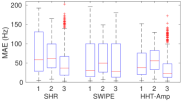


Fig. 5 and Fig. 6 illustrate the MAE results obtained for six noisy conditions with the CSTR and TIMIT databases, respectively. Each box-plot denotes the MAE values achieved with five SNR values: -15 dB, -10 dB, -5 dB, 0 dB and 5 dB. Note that again the proposed method achieved the lowest MAE values. For CSTR database, the DCNN strategy attains improvement in original F0 estimation in some cases of SHR and SWIPE, particularly for SSN, Cafeteria, and Helicopter noises. The MAE values for the TIMIT database indicate that PRO improved the F0 estimation accuracy, overcoming the DCNN baseline solution. Once again, the PRO method leads the HHT-Amp estimator to achieve best accuracy results for both databases, with exception for Volvo noise with TIMIT (Fig. 6(f)).
In summary, the proposed method leads to the best results when compared to the solution DCNN, in terms of low/high frequency separation accuracy, and improvement of fundamental frequency estimation accuracy. In addition, the combination of PRO with the HHT-Amp algorithm (PRO + HHT-Amp) attained the lowest GE and MAE scores, for both the CSTR and TIMIT databases. Furthermore, SHR baseline approach are also outperformed by the HHT-Amp. The fact that SHR adopts two F0 candidates, against the three candidates considered in HHT-Amp, can favor this last one in the true F0 selection. In contrast, baseline techniques based on the SWIPE estimation reach the highest error values. This occurs because SWIPE is very sensitive to the severe noise disturbances, which may cause expressive voiced/unvoiced detection errors. Finally, it is interesting to observe that even considering the classification errors in the estimation accuracy results, the proposed method improves F0 estimation of speech signals corrupted by different types of noise, and hence it can be used in real world applications.
| Original | DCNN | PRO | ||||||||
|---|---|---|---|---|---|---|---|---|---|---|
| SHR | SWIPE | HHT-Amp | SHR | SWIPE | HHT-Amp | SHR | SWIPE | HHT-Amp | ||
| 0.03 | 0.03 | 0.93 | 0.22 | 0.20 | 1.07 | 0.94 | 0.95 | 1.00 | ||
Table III indicates the computational complexity which refers to the normalized processing time required for each scheme evaluated for 512 samples per frame. These values are obtained with an Intel (R) Core (TM) i7-9700 CPU, 8 GB RAM, and are normalized by the execution time of the most accurate method PRO + HHT-Amp. The processing time required for the training process by DCNN is not considered here. Therefore, note that the HHT-Amp baseline scheme and the proposed method present a longer processing time, since they are based on the EEMD, and demands a relevant computational cost.
V Conclusion
This paper introduced a method for low/high frequency separation of voiced frames, in order to improve the F0 estimation accuracy. The EEMD algorithm was applied to decompose the noisy speech signal. Then, F0 estimation and selection of analyzed decomposition modes was performed to detect the low or high frequency region of the voiced frames. According to this separation, the candidates of F0 estimation techniques were corrected, improving their accuracy. Several experiments were conducted to evaluate the improvement provided by the PRO method and the DCNN based approach, with three baseline F0 estimation techniques. Two speech databases and six acoustic noises of different sources were adopted for this purpose. Results were examined considering separation accuracy, and estimation error measures GE and MAE. The proposed method attained the smallest errors in low/high frequency separation in all cases, when compared to DCNN. Furthermore, the F0 estimation metrics demonstrated that PRO leads to superior improvement in F0 estimation accuracy. Particularly, the PRO + HHT-Amp method outperformed the baseline approaches in terms of GE and MAE, with interesting accuracy in F0 detection in various noisy environments. Future research includes the investigation of the low/high frequency separation in other tasks, such as for intelligibility improvement.
References
- [1] L. Geurts and J. Wouters, “Coding of the fundamental frequency in continuous interleaved sampling processors for cochlear implants,” J. Acoust. Soc. Amer., vol. 109, no. 2, pp. 713–726, Feb. 2001.
- [2] K. N. Ross and M. Ostendorf, “A dynamical system model for generating fundamental frequency for speech synthesis,” IEEE Trans. Speech Audio Process., vol. 7, no. 3, pp. 295–309, May 1999.
- [3] M. R. Sambur, “Selection of acoustic features for speaker identification,” IEEE Trans. Acoust., Speech, Signal Process., vol. 23, no. 2, pp. 176–182, Apr. 1975.
- [4] A. Ljolj, “Speech recognition using fundamental frequency and voicing in acoustic modeling,” in Proc. Int. Conf. Spoken Lang. Process., 2002.
- [5] D. Ealey, H. Kelleher, , and D. Pearce, “Harmonic tunnelling: Tracking nonstationary noises during speech,” in Proc. 7th Eur. Conf. Speech Commun. Technol., pp. 437–440, 2001.
- [6] L. Wang and F. Chen, “Factors affecting the intelligibility of low-pass filtered speech,” in Proc. INTERSPEECH, pp. 563–566, Aug. 2017.
- [7] A. Queiroz and R. Coelho, “F0-based gammatone filtering for intelligibility gain of acoustic noisy signals,” IEEE Signal Process. Lett., vol. 28, pp. 1225–1229, 2021.
- [8] H. Traunmuller and A. Eriksson, “The perceptual evaluation of f0 excursions in speech as evidenced in liveliness estimations,” J. Acoust. Soc. Amer., vol. 97, no. 3, pp. 1905–1915, 1995.
- [9] C. Brown and S. Bacon, “Fundamental frequency and speech intelligibility in background noise,” Hear. Res., vol. 266, pp. 52–59, 2010.
- [10] L. Wang, D. Zheng, and F. Chen, “Understanding low-pass-filtered mandarin sentences: Effects of fundamental frequency contour and single-channel noise suppression,” J. Acoust. Soc. Amer., vol. 143, no. 3, pp. 141–145, 2018.
- [11] J. Dubnowski, R. Schafer, and L. Rabiner, “Real-time digital hardware pitch detector,” IEEE Trans. Acoust., Speech Signal Process., vol. 24, no. 1, pp. 2–8, 1976.
- [12] L. Rabiner, “On the use of autocorrelation analysis for pitch detection,” IEEE Trans. Acoust., Speech Signal Process., vol. 25, pp. 24–33, 1977.
- [13] A. de Cheveigné and H. Kawahara, “Yin, a fundamental frequency estimator for speech and music,” J. Acoust. Soc. Amer., vol. 111, no. 4, pp. 1917–1930, 2002.
- [14] X. Sun, “Pitch determination and voice quality analysis using subharmonic-to-harmonic ratio,” Proc. IEEE Int. Conf. Acoust., Speech, Signal Process., vol. 1, pp. I–333–I–336, 2002.
- [15] A. Camacho and J. G. Harris, “A sawtooth waveform inspired pitch estimator for speech and music,” J. Acoust. Soc. Amer., vol. 124, no. 3, pp. 1638–1652, 2008.
- [16] S. Gonzalez and M. Brookes, “A pitch estimation filter robust to high levels of noise (pefac),” Proceedings of the IEEE, pp. 451–455, 2011.
- [17] N. Yang, H. Ba, W. Cai, I. Demirkol, and W. Heinzelman, “Bana: A noise resilient fundamental frequency detection algorithm for speech and music,” IEEE/ACM Trans. Audio, Speech, Lang. Process., vol. 22, no. 12, pp. 1833–1848, 2014.
- [18] G. Aneeja and B. Yegnanarayana, “Extraction of fundamental frequency from degraded speech using temporal envelopes at high snr frequencies,” IEEE Trans. Audio, Speech, Lang. Process., vol. 25, no. 4, pp. 829–838, 2017.
- [19] Y. Liu, J. Tao, D. Zhang, and Y. Zheng, “A novel pitch extraction based on jointly trained deep blstm recurrent neural networks with bottleneck features,” Proc. IEEE Int. Conf. Acoust., Speech, Signal Process., pp. 336–340, 2017.
- [20] T. Drugman, G. Huybrechts, V. Klimkov, and A. Moinet, “Traditional machine learning for pitch detection,” IEEE Signal Process. Lett., vol. 25, no. 11, pp. 1745–1749, 2018.
- [21] J. Kim, J. Salamon, P. Li, and J. Bello, “Crepe: A convolutional representation for pitch estimation,” Proc. IEEE Int. Conf. Acoust., Speech, Signal Process., pp. 161–165, 2018.
- [22] B. Gfeller, C. Frank, D. Roblek, M. Sharifi, M. Tagliasacchi, and M. Velimirovic, “Spice: Self-supervised pitch estimation,” IEEE/ACM Trans. Audio, Speech, Lang. Process., vol. 28, pp. 1118–1128, 2020.
- [23] H. Hong, Z. Zhao, X. Wang, and Z. Tao, “Detection of dynamic structures of speech fundamental frequency in tonal languages,” IEEE Signal Process. Lett., vol. 17, no. 10, pp. 843–846, 2010.
- [24] L. Zão and R. Coelho, “On the estimation of fundamental frequency from nonstationary noisy speech signals based on hilbert-huang transform,” IEEE Signal Process. Lett., vol. 25, no. 2, pp. 248–252, 2018.
- [25] N. E. Huang, Z. Shen, S. R. Long, M. C. Wu, H. H. Shih, Q. Zheng, N. C. Yen, C. C. Tung, and H. H. Liu, “The empirical mode decomposition and the hilbert spectrum for nonlinear and non-stationary time series analysis,” Proc. Roy. Soc. London Ser. A: Math., Phys., Eng. Sci., vol. 454, no. 1971, pp. 903–995, 1998.
- [26] L. Zão, R. Coelho, and P. Flandrin, “Speech enhancement with emd and hurst-based mode selection,” IEEE/ACM Trans. Audio, Speech, Lang. Process., vol. 22, no. 5, pp. 897–909, 2014.
- [27] R. Coelho and L. Zão, “Empirical mode decomposition theory applied to speech enhancement,” in Signals and Images: Advances and Results in Speech, Estimation, Compression, Recognition, Filtering, and Processing, R.Coelho, V.Nascimento, R.Queiroz, J.Romano, and C.Cavalcante: Eds. Boca Raton, FL, USA: CRC Press, 2015.
- [28] A. Stallone, A. Cicone, and M. Materassi, “New insights and best practices for the successful use of empirical mode decomposition, iterative filtering and derived algorithms,” Nat. Sci. Rep., vol. 10, no. 15161, pp. 1–15, 2020.
- [29] D. Talkin, W. R. Kleiin, and K. K. Paliwal, “A robust algorithm for pitch tracking,” in Speech Coding and Synthsis, Elsevier, 1995.
- [30] B. Gfeller, C. Frank, D. Roblek, M. Sharifi, M. Tagliasacchi, and M. Velimirovic, “Error correction in pitch detection using a deep learning based classification,” IEEE/ACM Trans. Audio, Speech, Lang. Process., vol. 28, pp. 990–999, 2020.
- [31] M. E. Torres, M. A. Colominas, G. Schlotthauer, and P. Flandrin, “A complete ensemble empirical mode decomposition with adaptive noise,” Proc. IEEE Int. Conf. Acoust., Speech Signal Process., pp. 4144–4147, 2011.
- [32] P. Bagshaw, S. Hiller, and M. A. Jack, “Enhanced pitch tracking and the processing of f0 contours for computer aided intonation teaching,” Proc. EUROSPEECH-93., pp. 1003–1006, 1993.
- [33] J. Garofolo, L. Lamel, W. Fischer, J. Fiscus, D. Pallett, N. Dahlgren, and V. Zue, “Timit acoustic-phonetic continuous speech corpus,” in Linguist. Data Consortium, Philadelphia, PA, USA, 1993.
- [34] L. Rabiner, M. Cheng, A. Rosenberg, and C. McGonegal, “A comparative study of several pitch detection algorithms,” IEEE/ACM Trans. Acout., Speech, Signal Process., vol. 24, no. 5, pp. 399–418, 1976.
- [35] C. Willmott, S. Ackleson, R. Davis, J. Feddema, K. Klink, D. Legates, J. O’Donnell, and C. Rowe, “Statistics for the evaluation and comparison of models,” Journal of Geophysical Research, Sep. 1985.
- [36] Z. Wu and N. Huang, “Ensemble empirical mode decomposition: a noise-assisted data analysis method,” Advances in Adaptive Data Analysis, vol. 1, no. 1, pp. 1–41, 2009.
- [37] N. Huang, “Introduction to the hilbert-huang transform and its related mathematical problems,” in Hilbert-Huang Transform and its Applications, N. Huang and S. Shen: Eds. Singapore: World Sci. Publishing, 2014.
- [38] C. Medina, R. Coelho, and L. Zão, “Impulsive noise detection for speech enhancement in hht domain,” IEEE/ACM Trans. Audio, Speech, Lang. Process., vol. 29, pp. 2244–2253, 2021.
- [39] N. Chatlani and J. Soraghan, “Emd-based filtering (emdf) of low-frequency noise for speech enhancement,” IEEE Trans. Audio, Speech, Lang. Process., vol. 20, no. 4, pp. 1158–1166, 2012.
- [40] H. J. Steeneken and F. W. Geurtsen, “Description of the rsg-10 noise-database,” report IZF, vol. 3, 1988.
- [41] I. R. Titze, “Principles of voice production,” Englewood Cliffs: Prentice Hall.
- [42] K. Simonyan and A. Zisserman, “Very deep convolutional networks for large-scale image recognition,” Proc. ICLR., 2015.
- [43] S. Gonzalez, “Pitch of the core timit database set,” 2014.
- [44] J. Thiemann, N. Ito, and E. Vincent, “Demand: a collection of multi-channel recordings of acoustic noise in diverse environments,” Proc. Meetings Acoust., 2013.
- [45] R. Bachu, S. Kopparthi, B. Adapa, and B. Barkana, “Separation of voiced and unvoiced using zero crossing rate and energy of the speech signal,” ASEE Reg. Conf., pp. 1–7, 2008.