Next-to-Next-to-Leading-Order QCD Prediction for the Pion Form Factor
Abstract
We accomplish for the first time the two-loop computation of the leading-twist contribution
to the pion electromagnetic form factor by employing the effective field theory formalism rigorously.
The next-to-next-to-leading-order short-distance matching coefficient is determined by
evaluating the appropriate -point QCD amplitude with the modern multi-loop technique
and subsequently by implementing the ultraviolet renormalization and infrared subtractions
with the inclusion of evanescent operators.
The renormalization/factorization scale independence of the obtained form factor
is then validated explicitly at .
The yielding two-loop QCD correction to this fundamental quantity turns out to be numerically significant
at experimentally accessible momentum transfers.
We further demonstrate that the newly computed two-loop radiative correction is highly beneficial for
an improved determination of the leading-twist pion distribution amplitude.
I Introduction
It is generally accepted that the pion electromagnetic form factor (EMFF) is of paramount importance for probing the infrared structure of QCD scattering amplitudes of hard exclusive reactions at leading power and beyond and for unraveling the precise mechanisms that dictate the intricate nature of composite hadron systems. Advancing our understanding towards this gold-plated form factor is especially suitable for delivering deep and far-reaching insights into the delicate interplay between the emergent and Higgs mass generation mechanisms for such lightest pseudoscalar mesons as the Nambu-Goldstone modes of QCD. Historically, the systematic analysis of the pion form factor played an indispensable role in establishing the perturbative factorization formalism for the entire domain of exclusive hadronic processes with large momentum transfers Lepage and Brodsky (1979, 1980); Efremov and Radyushkin (1980a, b); Duncan and Mueller (1980a, b); Brodsky and Lepage (1989). As a consequence, the dimensional-counting rules for the power-law behaviour of numerous hard exclusive reactions on the basis of the parton model Brodsky and Farrar (1973); Matveev et al. (1973) can be placed on a solid footing within this field-theoretical framework (see Gross et al. (2023) for an overview). Additionally, the developed perturbative factorization technique has been extended to the first-principles calculations of the deeply virtual Compton scattering Ji (1997); Radyushkin (1997); Diehl et al. (1999a, b), the hard diffraction of light mesons at high energies Collins et al. (1997); Brodsky et al. (1994); Pire et al. (2021), and the exclusive heavy-to-light -meson decays at large hadronic recoil Beneke and Feldmann (2001, 2004); Bauer et al. (2001, 2003). Moreover, the time-like scalar-current pion form factors are intimately connected with the chirally-enhanced weak annihilation contributions to the flagship charmless two-body hadronic decays Beneke et al. (2001); Duraisamy and Kagan (2010); Lü et al. (2023), which provide an essential testing ground for CP violation in the Standard Model (SM) with controllable theoretical uncertainties.
Experimentally, the pion EMFF at low momentum transfers () has been measured from the elastic scattering of high-energy pions off the atomic electrons in a liquid-hydrogen target at Fermilab Dally et al. (1981, 1982) and CERN Amendolia et al. (1984, 1986). The challenging measurement of the pion form factor at intermediate momentum transfers, up to , has been further carried out at Cornell Bebek et al. (1976a, b, 1978), DESY Brauel et al. (1979); Ackermann et al. (1978) and JLab Volmer et al. (2001); Tadevosyan et al. (2007); Horn et al. (2006); Blok et al. (2008); Huber et al. (2008), by exploiting the so-called Sullivan mechanism and by extrapolating the determined longitudinal cross section at negative values of the Mandelstam variable to the pion pole at Sullivan (1972). Extracting the charged pion form factor over a wide range of the moderate momentum transfers () can be also anticipated from the E12-06-101 experiment with the upgraded JLab accelerator Arrington et al. (2022). Accessing the space-like pion form factor at yet higher momentum transfers () with high precision will be one of the key targets for the forthcoming EIC experiment at BNL Abdul Khalek et al. (2022).
According to the hard-collinear factorization theorem Lepage and Brodsky (1979, 1980); Efremov and Radyushkin (1980a, b); Duncan and Mueller (1980a, b), the leading-power contribution to the pion EMFF in the large-momentum expansion can be expressed in terms of the short-distance matching coefficient and the twist-two light-cone distribution amplitude (LCDA) for the (anti)-collinear pion state. The next-to-leading order (NLO) QCD correction to the perturbatively calculable hard function had been explicitly determined with the diagrammatic factorization approach more than forty years ago Field et al. (1981); Dittes and Radyushkin (1981); Sarmadi (1982); Khalmuradov and Radyushkin (1985); Braaten and Tse (1987) (see Melic et al. (1999) for further verification). Including the complete NLO radiative correction in the factorization analysis of the pion EMFF turns out to be extraordinarily advantageous to pin down the intrinsic theory uncertainty from varying the renormalization and factorization scales in comparison with the counterpart tree-level prediction Melic et al. (1999). Accomplishing the next-to-next-to-leading-order (NNLO) computation of the short-distance coefficient function rigorously is therefore in high demand, on the one hand, for enriching and developing the perturbative factorization formalism at an unprecedented level, and on the other hand, for improving further the resulting theory prediction of the charged pion form factor in order to match the ever-growing precision of the dedicated experimental measurements at JLab and EIC. It is our primary objective to fill such an important and longstanding gap in this Letter, by evaluating an appropriate -point partonic matrix element at with the contemporary advanced multi-loop computational strategies and by carrying out the ultraviolet (UV) renormalization and infrared (IR) subtractions in a meticulous and factorization-compatible manner CCF . Phenomenological implications of the thus determined two-loop QCD correction to the space-like pion form factor at large momentum transfers will be then explored comprehensively, by adopting four sample models for the leading-twist pion distribution amplitude at a low reference scale.
II General analysis
We first lay out the theoretical framework for constructing the hard-collinear factorization formula of the pion EMFF at leading power in an expansion in powers of , where stands for the strong interaction scale. Applying the general decomposition for the hadronic matrix element of the quark electromagnetic current enables us to write down
| (1) |
where and correspond to the four-momenta carried by the initial and final pion states, respectively. Employing the vector-current conservation condition immediately leads to , thus leaving us with a single form factor . Implementing further the charge conjugation transformation for the matrix element on the left-hand side of (1) indicates an isospin relation between the two charged pion form factors for an arbitrary value of . In addition, the electric charge conservation determines the normalization condition for the pion form factor in the forward-scattering limit (see, for instance, Khodjamirian (2020) for an elementary discussion). Here the customary notation has been employed and the quark electromagnetic current is given by
| (2) |
with and for the up and down quarks. Introducing two light-like reference vectors and with the constraints and then allows for the decomposition and at the leading-power accuracy.
Taking advantage of the modern effective theory field technique Bauer et al. (2002); Rothstein (2004), the hard-collinear factorization formula for the pion form factor at large momentum transfers can be cast in the desired form (see Li and Sterman (1992); Li et al. (2011, 2013, 2014); Li and Wang (2015) for an alternative formalism)
| (3) | |||||
which is valid to all orders in perturbation theory and at leading power in the expansion. We take the charged pion decay constant from the three-flavour FLAG average Aoki et al. (2022) with an increased uncertainty from adding an approximate charm sea-quark contribution. Apparently, the hard-scattering kernel depends on both the renormalization scale and the factorization scale , the latter of which corresponds to the resolution with which the microscopic structure of the -meson is being probed. This short-distance coefficient function can be expanded perturbatively in terms of the strong coupling constant (similarly for any other QCD quantity)
| (4) |
The leading-twist pion distribution amplitude in the factorized expression (3) can be defined by the renormalized QCD matrix element on the light-cone Braun and Filyanov (1989, 1990)
| (5) |
where is the finite-length collinear Wilson line ensuring gauge invariance. The one-loop renormalization-group (RG) equation for the light-ray operator on the left-hand side of (5) implies the conformal partial wave expansion of in terms of the Gegenbauer polynomials with multiplicatively renormalizable coefficients (see Braun et al. (2003) for an excellent overview)
| (6) |
The normalization condition has been adopted throughout this work and the odd moments vanish due to the -parity symmetry.
The short-distance matching coefficient can be routinely determined by investigating the -point QCD matrix element below
| (7) |
where the external momenta can be restricted to their leading components , , and with the “bar notation” , . We will perform the computation of the bare amplitude in dimensional regularization with , where UV and IR divergences manifest themselves as poles up to the second order in . The former divergences are evidently cancelled by the UV renormalization for the strong coupling constant in the scheme, while the latter disappear after executing the nowadays standard IR subtraction procedure.
III Next-to-next-to-leading-order QCD computation
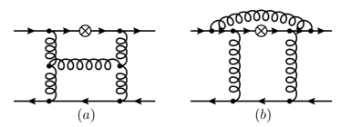
We will dedicate this section to a brief technical description of the two-loop QCD calculation for the considered partonic quantity . We start with generating the NNLO Feynman diagrams with FeynArts Hahn (2001) and, independently, by means of an in-house routine. Taking into account the observation that a subset of the two-loop diagrams yield the vanishing contribution, due to the Furry theorem and/or the zero colour (electric) charge factors, we eventually encounter non-vanishing diagrams of our interest. The two sample Feynman diagrams are depicted in Figure 1 explicitly.
All tensor integrals can be expressed in terms of scalar integrals and algebraic tensorial structures using the Passarino-Veltman decomposition Passarino and Veltman (1979). We then perform the Dirac and tensor reductions with in-house Mathematica routines, by applying further the QCD equations of motion and on-shell conditions. The large amount of two-loop scalar integrals are further reduced to an irreducible set of master integrals with the packages Apart Feng (2012) and FIRE Smirnov (2008). In total, we obtain two-loop master integrals that appear in our computation, of which appear to depend on physical scale(s). Unsurprisingly, we encounter the entire list of the one- and two-scale master integrals entering the NNLO computation of the photon-pion form factor Gao et al. (2022a, b). The evaluation of the remaining master integrals can be accomplished in an analytic fashion by employing the method of differential equations Kotikov (1991); Gehrmann and Remiddi (2000). In order to identify a suitable linear transformation such that the master integrals in the new basis satisfy a set of differential equations in an -factorized form (i.e., canonical form) Henn (2013), we take advantage of Lee’s algorithm Lee (2015) as implemented in the program Libra Lee (2021). The boundary conditions to the differential equations are determined by capitalizing on the package AMFlow Liu and Ma (2023) based upon Liu et al. (2018); Liu and Ma (2022). The yielding numerical results of the master integrals at three distinct kinematic points , with approximately digits, allow us to construct the desired boundary constants of the differential equations in terms of transcendental numbers using the PSLQ algorithm Ferguson et al. (1999, 1998). It is thus straightforward to express the master integrals through Goncharov polylogarithms (GPLs) Goncharov (1998, 2001) up to the required order in . We will present the analytic expressions for all master integrals in the forthcoming write-up.
IV Ultraviolet renormalization and infrared subtractions
We proceed to deduce the master formula for the hard-scattering kernel by performing the UV renormalization and IR subtractions in the presence of evanescent operators, whose significance in the perturbative treatment of quantum field theory has been explored at length ever since the pioneering era of dimensional regularization Breitenlohner and Maison (1977); Bonneau (1980a, b); Collins (2023). To achieve this goal, we exploit the matching equation for the interested QCD amplitude onto the effective matrix elements
| (8) |
with the following choice of the collinear operator basis
| (9) |
One can readily verify that is the only physical operator in our problem and the other two operators are evanescent, i.e., vanish algebraically in four dimensions. To reduce our notation to the essentials, we strip off the collinear Wilson lines and the position arguments of quark fields from , and represent them merely by their flavour and Dirac structure. Following the conventions of Beneke and Jager (2006), we label the collinear and anti-collinear effective fields moving into the directions of and by and , respectively, which evidently satisfy and .
We are now in a position to organize the perturbative expansion of the renormalized QCD correlation function in terms of the partonic tree-level matrix elements of the effective operators
| (10) | |||||
where the renormalization constant of the strong coupling in the standard scheme takes the form of (see Herzog et al. (2017); Luthe et al. (2017); Chetyrkin et al. (2017) for the five-loop expression). The scalar quantities in (10) represent the bare -loop on-shell QCD amplitudes. In the same vein, the UV-renormalized matrix elements of the collinear operators can be expanded according to
| (11) |
further taking into account that scaleless integrals vanish in dimensional regularization. Since the collinear fields for distinct directions already decouple at the hard scale, the renormalization constant can be therefore determined from the celebrated Efremov-Radyushkin-Brodske-Lepage (ERBL) kernel with the one- and two-loop results obtained in Lepage and Brodsky (1980); Efremov and Radyushkin (1980b) and Sarmadi (1984); Dittes and Radyushkin (1984); Katz (1985); Mikhailov and Radyushkin (1985); Belitsky et al. (1999). Substituting Eqs. (4), (10) and (11) into the matching equation (8) leads us to derive the master formulae for the short-distance coefficient function
| (12) | |||||
by comparing the coefficient of the tree-level matrix element of the physical operator . Following the prescription proposed in Dugan and Grinstein (1991); Herrlich and Nierste (1995); Buras and Weisz (1990); Jamin and Pich (1994); Buras (2023), the renormalization constants for the evanescent operators are adjusted to ensure that the IR-finite matrix elements () vanish at an arbitrary scale. Adopting the preferred collinear operator basis (9) yields the peculiar evanescent-to-physical operator mixing under the RG evolution, which turns out to be adequately captured by the finite renormalization constant at two-loop order. This justifies the essential role of introducing evanescent operators in constructing the QCD factorization formulae with dimensional regularization beyond the leading logarithmic approximation Beneke and Jager (2006, 2007); Becher and Hill (2004); Hill et al. (2004); Beneke and Yang (2006); Buchalla et al. (1996); Buras et al. (2000); Wang and Shen (2015, 2017); Gao et al. (2020, 2022a); Huang et al. (2024); Li et al. (2020); Cui et al. (2023).
Inserting the newly obtained two-loop expression of the hard-scattering kernel into the collinear factorization formula (3) and then performing the two-fold integration over and analytically with the Mathematica package PolyLogTools Duhr and Dulat (2019) in the asymptotic approximation (namely, ) results in
| (13) | |||||
where and denote the Casimir operators of the fundamental and adjoint representations of the gauge group with the standard normalization . In addition, stands for the number of active quark flavours, and represents the Riemann zeta function with , , , and Vermaseren (1999); Smirnov (2012). Including the higher conformal spin contributions from the twist-two pion LCDA leads to the lengthy results for the non-asymptotic corrections to the charged pion form factor, whose explicit expressions with the truncation of the Gegenbauer expansion are collected in the Supplemental Material for completeness. In particular, we have verified that the thus achieved NNLO QCD computation of with the perturbative factorization formula (3) is truly independent of the renormalization/factorization scale at the accuracy, by applying the two-loop evolution equation of Sarmadi (1984); Dittes and Radyushkin (1984); Katz (1985); Mikhailov and Radyushkin (1985); Belitsky et al. (1999). Taking advantage of the momentum-space RG formalism enables us to accomplish an all-order summation of the enhanced logarithms of entering the factorized expression of in the next-to-next-to-leading-logarithmic (NNLL) approximation, which necessitates an implementation of the three-loop evolution of the leading-twist pion distribution amplitude Braun et al. (2017); Strohmaier (2018).
V Numerical analysis
We are now prepared to explore the phenomenological implication of the newly determined two-loop QCD correction to the pion EMFF, with an emphasis on the detailed comparison with both the available experimental measurements and the state-of-the-art lattice QCD results. To achieve this goal, we proceed by first discussing our choice for the phenomenological models of the twist-two pion LCDA appearing in the hard-collinear factorization formula (3). The first model is motivated from the anti-de Sitter-QCD correspondence Brodsky and de Teramond (2008) with the non-perturbative parameter Khodjamirian et al. (2021) determined by matching to the updated lattice result of the second Gegenbauer moment at the reference scale Bali et al. (2019). Our second model Cheng et al. (2020) is obtained from the comparison of the light-cone sum rule for the pion EMFF Braun et al. (2000) with the experimental measurements (see Bijnens and Khodjamirian (2002); Khodjamirian et al. (2011) for the earlier construction along this line). By contrast, the numerical intervals for the two lowest conformal coefficients in model III Bakulev et al. (2001); Mikhailov et al. (2016); Stefanis (2020) are extracted from the method of QCD sum rules with non-local condensates Mikhailov and Radyushkin (1992). Furthermore, we employ an alternative model (hereafter labelled as model IV) with the first three non-vanishing Gegenbauer coefficients Cloet et al. (2024) determined from the lattice prediction for the dynamic shape of the pion distribution amplitude in the range of using large momentum effective theory Ji (2013, 2014); Ji et al. (2021) and from a simple power-law parametrization of the corresponding end-point behaviour. Additionally, we will vary the renormalization scale for the strong coupling in the interval with the central value . Following Agaev et al. (2011), the factorization scale characterizing the virtualities of quark and gluon propagators in the hard-scattering partonic process will be taken as with (see Melic et al. (1999, 2002); Stefanis (1999); Mojaza et al. (2013); He et al. (2006); Lu et al. (2009); Wang and Shen (2016, 2017); Di Giustino et al. (2024) for an elaborate discussion on the renormalization/factorization scale setting).
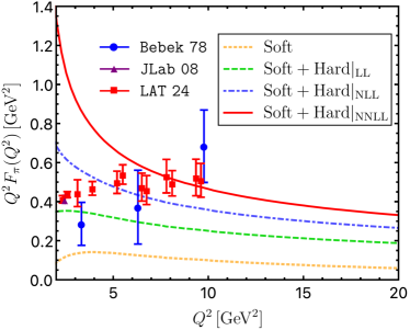
In order to facilitate an in-depth exploration of the dynamical pattern dictating the pion form factor, we display explicitly in Figure 2 the obtained theory predictions for the leading-power hard-gluon-exchange contributions at leading-logarithmic (LL), NLL, and NNLL accuracy accomplished in this Letter as well as the subleading power corrections arising from I) an atypical “end-point” configuration of twist-two in the one-loop approximation and II) the higher-twist pion distribution amplitudes up to the twist-six accuracy with the dispersion technique Braun et al. (2000), by adopting model I of the pion distribution amplitude as our default choice. Inspecting the distinctive feature for a variety of higher-order corrections in Figure 2 implies that the newly determined two-loop QCD correction to the hard-scattering contribution based upon the hard-collinear factorization theorem can substantially enhance the corresponding NLL prediction of the pion form factor at intermediate and large momentum transfers: numerically at the level of . In analogy to the QCD anatomy of the radiative leptonic decay with an energetic photon Braun and Khodjamirian (2013); Wang (2016); Wang and Shen (2018); Beneke et al. (2018); Khodjamirian et al. (2024), the soft non-factorizable correction to the charged pion form factor can constantly shift the NNLL resummation improved leading-power contribution by approximately an amount of in the kinematic domain . We are then led to conclude that an ironclad and fully analytical extraction of the two-loop short-distance coefficient function in the factorized expression (3) is evidently vital for obtaining the robust and accurate theory prediction of the flagship hadron form factor and for advancing further the QCD factorization programme targeting at the high-precision computation of hard exclusive reactions. It remains interesting to observe that the very inclusion of the NNLO QCD correction to the pion EMFF turns out to be especially beneficial for better accommodating the benchmark lattice simulation results at intermediate momentum transfers Ding et al. (2024).
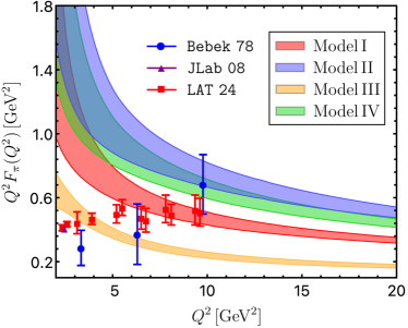
We now turn to present in Figure 3 our final theory predictions for the pion form factor with the four different phenomenological models of the twist-two pion LCDA discussed above, confronting with the two experimental measurements Bebek 78 Bebek et al. (1978) and JLab 08 Huber et al. (2008) at four distinct kinematic points of . It can then be observed that the yielding numerical prediction with the anti-de Sitter-QCD inspired model fulfilling an additional constraint from the lattice determination of Bali et al. (2019) (i.e., our model I) provides us with the most optimized description of the available experimental data points and the model-independent lattice QCD results Ding et al. (2024) simultaneously. The extraordinary snapshot of the well-separated uncertainty bands for the first three sample models due to the variations of the renormalization/factorization scales in the preferred intervals is particularly encouraging to acquire new insights on the intricate behaviour of the leading-twist pion distribution amplitude, in combination with the envisaged precision measurements at JLab and EIC. In contrast with the NNLL QCD computation for the photon-pion transition form factor Gao et al. (2022a); Braun et al. (2021), our two-loop prediction of the pion EMFF based upon the hard-collinear factorization prescription approaches the desired scaling behaviour in the formal limit rather slowly. This intriguing pattern can be attributed to the fact that the determined hierarchy between the subleading conformal spin effect and the counterpart asymptotic contribution grows steadily with the increasing loop order at realistic momentum transfers accessible in the current and forthcoming experimental facilities, thus postponing the onset of the asymptotic regime to an enormously higher value of (see Braun et al. (2002, 2006); Anikin et al. (2013); Huang et al. (2024) for further discussions in the context of the nucleon electromagnetic form factors).
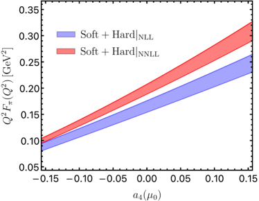
We finally address the genuine benefit of the full two-loop QCD calculation of the charged pion form factor on the model-independent extraction of the shape parameters dictating the twist-two pion distribution amplitude on the light-cone. To this end, we proceed to explore the intrinsic sensitivity of the exclusive form factor on the currently poorly constrained conformal coefficient by combining the achieved NNLL prediction of the leading-twist contribution with the previously determined subleading power corrections in the expansion. It is evident from Figure 4 that taking into account the newly obtained two-loop QCD correction to the pion EMFF form factor will indeed be advantageous to enhance the sensitivity of extracting the key shape parameter in anticipation of the prospective precision EIC measurements Abdul Khalek et al. (2022), complementary to an alternative strategy on the basis of the factorization analysis of the photon-pion form factor Gao et al. (2022a).
VI Conclusions
In conclusion, we have endeavored to accomplish for the first time the rigorous two-loop QCD computation of the pion form factor in an analytical fashion, by applying the modern effective field theory formalism that enables us to implement the UV renormalization and IR subtractions of evanescent operators systematically. Crucially, we have demonstrated that the thus determined NNLO QCD correction to the short-distance coefficient function can bring about an enormous impact on the pion form factor over a wide range of momentum transfers, by employing the four phenomenologically acceptable models of the leading-twist pion distribution amplitude. In particular, the very inclusion of the two-loop radiative correction allowed for an improved extraction of the essential shape parameters dictating the intricate profile of the pion distribution amplitude, when confronted with the encouraging measurements from the upcoming EIC experiment. Extending and developing further our factorization prescription to the charged kaon form factor and to the more challenging transition form factors Böer (2018); Bell and Feldmann (2007); Bell (2006); Böer et al. (2024) will be highly beneficial for deepening our understanding towards the diverse facets of the strong interaction dynamics encoded in the hard-scattering processes.
Acknowledgements.
Acknowledgements
It is our pleasure to thank Yong-Kang Huang for illuminating discussions. The research of Y.J. was supported in part by the Deutsche Forschungsgemeinschaft (DFG, German Research Foundation) through the Sino-German Collaborative Research Center TRR110 “Symmetries and the Emergence of Structure in QCD” (DFG Project-ID 196253076, NSFC Grant No. 12070131001, - TRR 110). J.W. is supported by the National Natural Science Foundation of China with Grant No. 12005117, No. 12321005, and No. 12375076, and the Taishan Scholar Foundation of Shandong province with Grant No. TSQN201909011. The work of Y.F.W. is supported in part by the National Natural Science Foundation of China with Grant No. 12405117. Y.M.W. acknowledges support from the National Natural Science Foundation of China with Grant No. 12075125 and No. 2475097.
Appendix A SUPPLEMENTAL MATERIAL
Here we collect the general expression for the derived two-loop pion electromagnetic form factor with the inclusion of the non-asymptotic corrections
| (14) | |||||
by inserting the Gegenbauer expansion of the pion distribution amplitude (6) into the hard-collinear factorization formula (3) and then by evaluating the double convolution integrals over the quark momentum fractions analytically. We can readily verify that the two coefficient matrices and coincide with the one- and two-loop anomalous dimensions (apart from an overall minus sign) of the flavour-octet local operators defining the conformal moments of the twist-two distribution amplitude . The explicit expressions of these anomalous dimensions are given by Mueller (1994)
| (15) |
where we have introduced the following definitions and conventions Braun et al. (2017); Strohmaier (2018); Belitsky and Radyushkin (2005)
| (18) |
It is straightforward to express the diagonal two-loop anomalous dimensions in terms of the preceding harmonic sums
| (19) | |||||
The non-trivial matrix arises from the one-loop conformal anomaly Braun et al. (2017)
| (20) |
where
| (21) |
We now turn to present the desired expressions for the scattering kernels and by truncating the Gegenbauer expansion (6) at (which is sufficient for practical purposes)
| (22) | ||||||
| (23) |
and
| (24) | ||||
| (25) |
It remains important to point out the interesting relations and on account of the charge-conjugation symmetry of the pion form factor.
References
- Lepage and Brodsky (1979) G. P. Lepage and S. J. Brodsky, Phys. Lett. B 87, 359 (1979).
- Lepage and Brodsky (1980) G. P. Lepage and S. J. Brodsky, Phys. Rev. D 22, 2157 (1980).
- Efremov and Radyushkin (1980a) A. V. Efremov and A. V. Radyushkin, Theor. Math. Phys. 42, 97 (1980a).
- Efremov and Radyushkin (1980b) A. V. Efremov and A. V. Radyushkin, Phys. Lett. B 94, 245 (1980b).
- Duncan and Mueller (1980a) A. Duncan and A. H. Mueller, Phys. Rev. D 21, 1636 (1980a).
- Duncan and Mueller (1980b) A. Duncan and A. H. Mueller, Phys. Lett. B 90, 159 (1980b).
- Brodsky and Lepage (1989) S. J. Brodsky and G. P. Lepage, Adv. Ser. Direct. High Energy Phys. 5, 93 (1989).
- Brodsky and Farrar (1973) S. J. Brodsky and G. R. Farrar, Phys. Rev. Lett. 31, 1153 (1973).
- Matveev et al. (1973) V. A. Matveev, R. M. Muradian, and A. N. Tavkhelidze, Lett. Nuovo Cim. 7, 719 (1973).
- Gross et al. (2023) F. Gross et al., Eur. Phys. J. C 83, 1125 (2023), arXiv:2212.11107 [hep-ph] .
- Ji (1997) X.-D. Ji, Phys. Rev. D 55, 7114 (1997), arXiv:hep-ph/9609381 .
- Radyushkin (1997) A. V. Radyushkin, Phys. Rev. D 56, 5524 (1997), arXiv:hep-ph/9704207 .
- Diehl et al. (1999a) M. Diehl, T. Feldmann, R. Jakob, and P. Kroll, Phys. Lett. B 460, 204 (1999a), arXiv:hep-ph/9903268 .
- Diehl et al. (1999b) M. Diehl, T. Feldmann, R. Jakob, and P. Kroll, Eur. Phys. J. C 8, 409 (1999b), arXiv:hep-ph/9811253 .
- Collins et al. (1997) J. C. Collins, L. Frankfurt, and M. Strikman, Phys. Rev. D 56, 2982 (1997), arXiv:hep-ph/9611433 .
- Brodsky et al. (1994) S. J. Brodsky, L. Frankfurt, J. F. Gunion, A. H. Mueller, and M. Strikman, Phys. Rev. D 50, 3134 (1994), arXiv:hep-ph/9402283 .
- Pire et al. (2021) B. Pire, K. Semenov-Tian-Shansky, and L. Szymanowski, Phys. Rept. 940, 1 (2021), arXiv:2103.01079 [hep-ph] .
- Beneke and Feldmann (2001) M. Beneke and T. Feldmann, Nucl. Phys. B 592, 3 (2001), arXiv:hep-ph/0008255 .
- Beneke and Feldmann (2004) M. Beneke and T. Feldmann, Nucl. Phys. B 685, 249 (2004), arXiv:hep-ph/0311335 .
- Bauer et al. (2001) C. W. Bauer, S. Fleming, D. Pirjol, and I. W. Stewart, Phys. Rev. D 63, 114020 (2001), arXiv:hep-ph/0011336 .
- Bauer et al. (2003) C. W. Bauer, D. Pirjol, and I. W. Stewart, Phys. Rev. D 67, 071502 (2003), arXiv:hep-ph/0211069 .
- Beneke et al. (2001) M. Beneke, G. Buchalla, M. Neubert, and C. T. Sachrajda, Nucl. Phys. B 606, 245 (2001), arXiv:hep-ph/0104110 .
- Duraisamy and Kagan (2010) M. Duraisamy and A. L. Kagan, Eur. Phys. J. C 70, 921 (2010), arXiv:0812.3162 [hep-ph] .
- Lü et al. (2023) C.-D. Lü, Y.-L. Shen, C. Wang, and Y.-M. Wang, Nucl. Phys. B 990, 116175 (2023), arXiv:2202.08073 [hep-ph] .
- Dally et al. (1981) E. B. Dally et al., Phys. Rev. D 24, 1718 (1981).
- Dally et al. (1982) E. B. Dally et al., Phys. Rev. Lett. 48, 375 (1982).
- Amendolia et al. (1984) S. R. Amendolia et al., Phys. Lett. B 146, 116 (1984).
- Amendolia et al. (1986) S. R. Amendolia et al. (NA7), Nucl. Phys. B 277, 168 (1986).
- Bebek et al. (1976a) C. J. Bebek, C. N. Brown, M. Herzlinger, S. D. Holmes, C. A. Lichtenstein, F. M. Pipkin, S. Raither, and L. K. Sisterson, Phys. Rev. D 13, 25 (1976a).
- Bebek et al. (1976b) C. J. Bebek et al., Phys. Rev. Lett. 37, 1326 (1976b).
- Bebek et al. (1978) C. J. Bebek et al., Phys. Rev. D 17, 1693 (1978).
- Brauel et al. (1979) P. Brauel, T. Canzler, D. Cords, R. Felst, G. Grindhammer, M. Helm, W. D. Kollmann, H. Krehbiel, and M. Schadlich, Z. Phys. C 3, 101 (1979).
- Ackermann et al. (1978) H. Ackermann, T. Azemoon, W. Gabriel, H. D. Mertiens, H. D. Reich, G. Specht, F. Janata, and D. Schmidt, Nucl. Phys. B 137, 294 (1978).
- Volmer et al. (2001) J. Volmer et al. (Jefferson Lab F(pi)), Phys. Rev. Lett. 86, 1713 (2001), arXiv:nucl-ex/0010009 .
- Tadevosyan et al. (2007) V. Tadevosyan et al. (Jefferson Lab F(pi)), Phys. Rev. C 75, 055205 (2007), arXiv:nucl-ex/0607007 .
- Horn et al. (2006) T. Horn et al. (Jefferson Lab F(pi)-2), Phys. Rev. Lett. 97, 192001 (2006), arXiv:nucl-ex/0607005 .
- Blok et al. (2008) H. P. Blok et al. (Jefferson Lab), Phys. Rev. C 78, 045202 (2008), arXiv:0809.3161 [nucl-ex] .
- Huber et al. (2008) G. M. Huber et al. (Jefferson Lab), Phys. Rev. C 78, 045203 (2008), arXiv:0809.3052 [nucl-ex] .
- Sullivan (1972) J. D. Sullivan, Phys. Rev. D 5, 1732 (1972).
- Arrington et al. (2022) J. Arrington et al., Prog. Part. Nucl. Phys. 127, 103985 (2022), arXiv:2112.00060 [nucl-ex] .
- Abdul Khalek et al. (2022) R. Abdul Khalek et al., Nucl. Phys. A 1026, 122447 (2022), arXiv:2103.05419 [physics.ins-det] .
- Field et al. (1981) R. D. Field, R. Gupta, S. Otto, and L. Chang, Nucl. Phys. B 186, 429 (1981).
- Dittes and Radyushkin (1981) F. M. Dittes and A. V. Radyushkin, Sov. J. Nucl. Phys. 34, 293 (1981).
- Sarmadi (1982) M. H. Sarmadi, The asymptotic pion form factor to the leading order and beyond, Ph.d. thesis (1982).
- Khalmuradov and Radyushkin (1985) R. S. Khalmuradov and A. V. Radyushkin, Sov. J. Nucl. Phys. 42, 289 (1985).
- Braaten and Tse (1987) E. Braaten and S.-M. Tse, Phys. Rev. D 35, 2255 (1987).
- Melic et al. (1999) B. Melic, B. Nizic, and K. Passek, Phys. Rev. D 60, 074004 (1999), arXiv:hep-ph/9802204 .
- (48) We note that an earlier attempt to carry out the two-loop QCD computation of the pion electromagnetic form factor at leading power in the expansion was made in the work Chen et al. (2024), by applying the light-cone projections on the leading-twist (anti)-collinear operators before performing the UV renormalization for the bare -point QCD matrix element. As extensively discussed in the factorization analysis of exclusive heavy-quark hadron decays Beneke and Jager (2006, 2007); Becher and Hill (2004); Hill et al. (2004); Beneke and Yang (2006), such projections do not necessarily commute with the renormalization for the considered bare QCD amplitude. Consequently, the practical prescription implemented in Chen et al. (2024) cannot be rigorously justified in the perturbative factorization framework (see Buchalla et al. (1996); Buras et al. (2000); Wang and Shen (2015, 2017); Gao et al. (2020, 2022a); Huang et al. (2024); Li et al. (2020); Cui et al. (2023); Aebischer et al. (2023); Buchoff and Wagman (2016) for additional discussions). In particular, it is insufficient to provide the results of the short-distance matching coefficients in the operator-product-expansion programme without specifying the very definition of evanescent operators, as already emphasized in the comprehensive textbooks Buras (2020); Collins (2023). Moreover, these authors failed to demonstrate the renormalization/factorization scale independence of the obtained pion form factor at two-loop order, since they did not take into account the UV renormalization of the strong coupling constant in an appopriate manner in the published version of Chen et al. (2024). In the revised preprint version https://arxiv.org/pdf/2312.17228, the authors explicitly admitted that they made this mistake in extracting the renormalized hard matching coefficient at , thus affecting the obtained numerical prediction for the two-loop QCD correction to the pion form factor substantially.
- Khodjamirian (2020) A. Khodjamirian, Hadron Form Factors: From Basic Phenomenology to QCD Sum Rules (CRC Press, 2020).
- Bauer et al. (2002) C. W. Bauer, S. Fleming, D. Pirjol, I. Z. Rothstein, and I. W. Stewart, Phys. Rev. D 66, 014017 (2002), arXiv:hep-ph/0202088 .
- Rothstein (2004) I. Z. Rothstein, Phys. Rev. D 70, 054024 (2004), arXiv:hep-ph/0301240 .
- Li and Sterman (1992) H.-n. Li and G. F. Sterman, Nucl. Phys. B 381, 129 (1992).
- Li et al. (2011) H.-n. Li, Y.-L. Shen, Y.-M. Wang, and H. Zou, Phys. Rev. D 83, 054029 (2011), arXiv:1012.4098 [hep-ph] .
- Li et al. (2013) H.-N. Li, Y.-L. Shen, and Y.-M. Wang, JHEP 02, 008 (2013), arXiv:1210.2978 [hep-ph] .
- Li et al. (2014) H.-N. Li, Y.-L. Shen, and Y.-M. Wang, JHEP 01, 004 (2014), arXiv:1310.3672 [hep-ph] .
- Li and Wang (2015) H.-n. Li and Y.-M. Wang, JHEP 06, 013 (2015), arXiv:1410.7274 [hep-ph] .
- Aoki et al. (2022) Y. Aoki et al. (Flavour Lattice Averaging Group (FLAG)), Eur. Phys. J. C 82, 869 (2022), arXiv:2111.09849 [hep-lat] .
- Braun and Filyanov (1989) V. M. Braun and I. E. Filyanov, Z. Phys. C 44, 157 (1989).
- Braun and Filyanov (1990) V. M. Braun and I. E. Filyanov, Z. Phys. C 48, 239 (1990).
- Braun et al. (2003) V. M. Braun, G. P. Korchemsky, and D. Müller, Prog. Part. Nucl. Phys. 51, 311 (2003), arXiv:hep-ph/0306057 .
- Hahn (2001) T. Hahn, Comput. Phys. Commun. 140, 418 (2001), arXiv:hep-ph/0012260 .
- Passarino and Veltman (1979) G. Passarino and M. J. G. Veltman, Nucl. Phys. B 160, 151 (1979).
- Feng (2012) F. Feng, Comput. Phys. Commun. 183, 2158 (2012), arXiv:1204.2314 [hep-ph] .
- Smirnov (2008) A. V. Smirnov, JHEP 10, 107 (2008), arXiv:0807.3243 [hep-ph] .
- Gao et al. (2022a) J. Gao, T. Huber, Y. Ji, and Y.-M. Wang, Phys. Rev. Lett. 128, 062003 (2022a), arXiv:2106.01390 [hep-ph] .
- Gao et al. (2022b) J. Gao, T. Huber, Y. Ji, and Y.-M. Wang, SciPost Phys. Proc. 7, 022 (2022b), arXiv:2110.14776 [hep-ph] .
- Kotikov (1991) A. V. Kotikov, Phys. Lett. B 254, 158 (1991).
- Gehrmann and Remiddi (2000) T. Gehrmann and E. Remiddi, Nucl. Phys. B 580, 485 (2000), arXiv:hep-ph/9912329 .
- Henn (2013) J. M. Henn, Phys. Rev. Lett. 110, 251601 (2013), arXiv:1304.1806 [hep-th] .
- Lee (2015) R. N. Lee, JHEP 04, 108 (2015), arXiv:1411.0911 [hep-ph] .
- Lee (2021) R. N. Lee, Comput. Phys. Commun. 267, 108058 (2021), arXiv:2012.00279 [hep-ph] .
- Liu and Ma (2023) X. Liu and Y.-Q. Ma, Comput. Phys. Commun. 283, 108565 (2023), arXiv:2201.11669 [hep-ph] .
- Liu et al. (2018) X. Liu, Y.-Q. Ma, and C.-Y. Wang, Phys. Lett. B 779, 353 (2018), arXiv:1711.09572 [hep-ph] .
- Liu and Ma (2022) X. Liu and Y.-Q. Ma, Phys. Rev. D 105, L051503 (2022), arXiv:2107.01864 [hep-ph] .
- Ferguson et al. (1999) H. Ferguson, D. Bailey, and S. Arno, Mathematics of Computation 68, 351 (1999).
- Ferguson et al. (1998) H. R. Ferguson, D. H. Bailey, and P. Kutler, A polynomial time, numerically stable integer relation algorithm, Tech. Rep. (1998).
- Goncharov (1998) A. B. Goncharov, Math. Res. Lett. 5, 497 (1998), arXiv:1105.2076 [math.AG] .
- Goncharov (2001) A. B. Goncharov, (2001), arXiv:math/0103059 .
- Breitenlohner and Maison (1977) P. Breitenlohner and D. Maison, Commun. Math. Phys. 52, 11 (1977).
- Bonneau (1980a) G. Bonneau, Nucl. Phys. B 167, 261 (1980a).
- Bonneau (1980b) G. Bonneau, Nucl. Phys. B 171, 477 (1980b).
- Collins (2023) J. C. Collins, Renormalization, Cambridge Monographs on Mathematical Physics, Vol. 26 (Cambridge University Press, Cambridge, 2023).
- Beneke and Jager (2006) M. Beneke and S. Jager, Nucl. Phys. B 751, 160 (2006), arXiv:hep-ph/0512351 .
- Herzog et al. (2017) F. Herzog, B. Ruijl, T. Ueda, J. A. M. Vermaseren, and A. Vogt, JHEP 02, 090 (2017), arXiv:1701.01404 [hep-ph] .
- Luthe et al. (2017) T. Luthe, A. Maier, P. Marquard, and Y. Schroder, JHEP 10, 166 (2017), arXiv:1709.07718 [hep-ph] .
- Chetyrkin et al. (2017) K. G. Chetyrkin, G. Falcioni, F. Herzog, and J. A. M. Vermaseren, JHEP 10, 179 (2017), [Addendum: JHEP 12, 006 (2017)], arXiv:1709.08541 [hep-ph] .
- Sarmadi (1984) M. H. Sarmadi, Phys. Lett. B 143, 471 (1984).
- Dittes and Radyushkin (1984) F. M. Dittes and A. V. Radyushkin, Phys. Lett. B 134, 359 (1984).
- Katz (1985) G. R. Katz, Phys. Rev. D 31, 652 (1985).
- Mikhailov and Radyushkin (1985) S. V. Mikhailov and A. V. Radyushkin, Nucl. Phys. B 254, 89 (1985).
- Belitsky et al. (1999) A. V. Belitsky, D. Mueller, and A. Freund, Phys. Lett. B 461, 270 (1999), arXiv:hep-ph/9904477 .
- Dugan and Grinstein (1991) M. J. Dugan and B. Grinstein, Phys. Lett. B 256, 239 (1991).
- Herrlich and Nierste (1995) S. Herrlich and U. Nierste, Nucl. Phys. B 455, 39 (1995), arXiv:hep-ph/9412375 .
- Buras and Weisz (1990) A. J. Buras and P. H. Weisz, Nucl. Phys. B 333, 66 (1990).
- Jamin and Pich (1994) M. Jamin and A. Pich, Nucl. Phys. B 425, 15 (1994), arXiv:hep-ph/9402363 .
- Buras (2023) A. J. Buras, Phys. Rept. 1025 (2023), 10.1016/j.physrep.2023.07.002, arXiv:1102.5650 [hep-ph] .
- Beneke and Jager (2007) M. Beneke and S. Jager, Nucl. Phys. B 768, 51 (2007), arXiv:hep-ph/0610322 .
- Becher and Hill (2004) T. Becher and R. J. Hill, JHEP 10, 055 (2004), arXiv:hep-ph/0408344 .
- Hill et al. (2004) R. J. Hill, T. Becher, S. J. Lee, and M. Neubert, JHEP 07, 081 (2004), arXiv:hep-ph/0404217 .
- Beneke and Yang (2006) M. Beneke and D. Yang, Nucl. Phys. B 736, 34 (2006), arXiv:hep-ph/0508250 .
- Buchalla et al. (1996) G. Buchalla, A. J. Buras, and M. E. Lautenbacher, Rev. Mod. Phys. 68, 1125 (1996), arXiv:hep-ph/9512380 .
- Buras et al. (2000) A. J. Buras, M. Misiak, and J. Urban, Nucl. Phys. B 586, 397 (2000), arXiv:hep-ph/0005183 .
- Wang and Shen (2015) Y.-M. Wang and Y.-L. Shen, Nucl. Phys. B 898, 563 (2015), arXiv:1506.00667 [hep-ph] .
- Wang and Shen (2017) Y.-M. Wang and Y.-L. Shen, JHEP 12, 037 (2017), arXiv:1706.05680 [hep-ph] .
- Gao et al. (2020) J. Gao, C.-D. Lü, Y.-L. Shen, Y.-M. Wang, and Y.-B. Wei, Phys. Rev. D 101, 074035 (2020), arXiv:1907.11092 [hep-ph] .
- Huang et al. (2024) Y.-K. Huang, B.-X. Shi, Y.-M. Wang, and X.-C. Zhao, (2024), arXiv:2407.18724 [hep-ph] .
- Li et al. (2020) H.-D. Li, C.-D. Lü, C. Wang, Y.-M. Wang, and Y.-B. Wei, JHEP 04, 023 (2020), arXiv:2002.03825 [hep-ph] .
- Cui et al. (2023) B.-Y. Cui, Y.-K. Huang, Y.-M. Wang, and X.-C. Zhao, Phys. Rev. D 108, L071504 (2023), arXiv:2301.12391 [hep-ph] .
- Duhr and Dulat (2019) C. Duhr and F. Dulat, JHEP 08, 135 (2019), arXiv:1904.07279 [hep-th] .
- Vermaseren (1999) J. A. M. Vermaseren, Int. J. Mod. Phys. A 14, 2037 (1999), arXiv:hep-ph/9806280 .
- Smirnov (2012) V. A. Smirnov, Analytic tools for Feynman integrals, Vol. 250 (2012).
- Braun et al. (2017) V. M. Braun, A. N. Manashov, S. Moch, and M. Strohmaier, JHEP 06, 037 (2017), arXiv:1703.09532 [hep-ph] .
- Strohmaier (2018) M. Strohmaier, Conformal symmetry breaking and evolution equations in Quantum Chromodynamics, Ph.D. thesis, Regensburg U. (2018).
- Brodsky and de Teramond (2008) S. J. Brodsky and G. F. de Teramond, Phys. Rev. D 77, 056007 (2008), arXiv:0707.3859 [hep-ph] .
- Khodjamirian et al. (2021) A. Khodjamirian, B. Melić, Y.-M. Wang, and Y.-B. Wei, JHEP 03, 016 (2021), arXiv:2011.11275 [hep-ph] .
- Bali et al. (2019) G. S. Bali, V. M. Braun, S. Bürger, M. Göckeler, M. Gruber, F. Hutzler, P. Korcyl, A. Schäfer, A. Sternbeck, and P. Wein (RQCD), JHEP 08, 065 (2019), [Addendum: JHEP 11, 037 (2020)], arXiv:1903.08038 [hep-lat] .
- Cheng et al. (2020) S. Cheng, A. Khodjamirian, and A. V. Rusov, Phys. Rev. D 102, 074022 (2020), arXiv:2007.05550 [hep-ph] .
- Braun et al. (2000) V. M. Braun, A. Khodjamirian, and M. Maul, Phys. Rev. D 61, 073004 (2000), arXiv:hep-ph/9907495 .
- Bijnens and Khodjamirian (2002) J. Bijnens and A. Khodjamirian, Eur. Phys. J. C 26, 67 (2002), arXiv:hep-ph/0206252 .
- Khodjamirian et al. (2011) A. Khodjamirian, T. Mannel, N. Offen, and Y. M. Wang, Phys. Rev. D 83, 094031 (2011), arXiv:1103.2655 [hep-ph] .
- Bakulev et al. (2001) A. P. Bakulev, S. V. Mikhailov, and N. G. Stefanis, Phys. Lett. B 508, 279 (2001), [Erratum: Phys.Lett.B 590, 309–310 (2004)], arXiv:hep-ph/0103119 .
- Mikhailov et al. (2016) S. V. Mikhailov, A. V. Pimikov, and N. G. Stefanis, Phys. Rev. D 93, 114018 (2016), arXiv:1604.06391 [hep-ph] .
- Stefanis (2020) N. G. Stefanis, Phys. Rev. D 102, 034022 (2020), arXiv:2006.10576 [hep-ph] .
- Mikhailov and Radyushkin (1992) S. V. Mikhailov and A. V. Radyushkin, Phys. Rev. D 45, 1754 (1992).
- Cloet et al. (2024) I. Cloet, X. Gao, S. Mukherjee, S. Syritsyn, N. Karthik, P. Petreczky, R. Zhang, and Y. Zhao, (2024), arXiv:2407.00206 [hep-lat] .
- Ji (2013) X. Ji, Phys. Rev. Lett. 110, 262002 (2013), arXiv:1305.1539 [hep-ph] .
- Ji (2014) X. Ji, Sci. China Phys. Mech. Astron. 57, 1407 (2014), arXiv:1404.6680 [hep-ph] .
- Ji et al. (2021) X. Ji, Y.-S. Liu, Y. Liu, J.-H. Zhang, and Y. Zhao, Rev. Mod. Phys. 93, 035005 (2021), arXiv:2004.03543 [hep-ph] .
- Agaev et al. (2011) S. S. Agaev, V. M. Braun, N. Offen, and F. A. Porkert, Phys. Rev. D 83, 054020 (2011), arXiv:1012.4671 [hep-ph] .
- Melic et al. (2002) B. Melic, B. Nizic, and K. Passek, Phys. Rev. D 65, 053020 (2002), arXiv:hep-ph/0107295 .
- Stefanis (1999) N. G. Stefanis, Eur. Phys. J. direct 1, 7 (1999), arXiv:hep-ph/9911375 .
- Mojaza et al. (2013) M. Mojaza, S. J. Brodsky, and X.-G. Wu, Phys. Rev. Lett. 110, 192001 (2013), arXiv:1212.0049 [hep-ph] .
- He et al. (2006) X.-G. He, T. Li, X.-Q. Li, and Y.-M. Wang, Phys. Rev. D 74, 034026 (2006), arXiv:hep-ph/0606025 .
- Lu et al. (2009) C.-D. Lu, Y.-M. Wang, H. Zou, A. Ali, and G. Kramer, Phys. Rev. D 80, 034011 (2009), arXiv:0906.1479 [hep-ph] .
- Wang and Shen (2016) Y.-M. Wang and Y.-L. Shen, JHEP 02, 179 (2016), arXiv:1511.09036 [hep-ph] .
- Di Giustino et al. (2024) L. Di Giustino, S. J. Brodsky, P. G. Ratcliffe, X.-G. Wu, and S.-Q. Wang, Prog. Part. Nucl. Phys. 135, 104092 (2024), arXiv:2307.03951 [hep-ph] .
- Ding et al. (2024) H.-T. Ding, X. Gao, A. D. Hanlon, S. Mukherjee, P. Petreczky, Q. Shi, S. Syritsyn, R. Zhang, and Y. Zhao, Phys. Rev. Lett. 133, 181902 (2024), arXiv:2404.04412 [hep-lat] .
- Braun and Khodjamirian (2013) V. M. Braun and A. Khodjamirian, Phys. Lett. B 718, 1014 (2013), arXiv:1210.4453 [hep-ph] .
- Wang (2016) Y.-M. Wang, JHEP 09, 159 (2016), arXiv:1606.03080 [hep-ph] .
- Wang and Shen (2018) Y.-M. Wang and Y.-L. Shen, JHEP 05, 184 (2018), arXiv:1803.06667 [hep-ph] .
- Beneke et al. (2018) M. Beneke, V. M. Braun, Y. Ji, and Y.-B. Wei, JHEP 07, 154 (2018), arXiv:1804.04962 [hep-ph] .
- Khodjamirian et al. (2024) A. Khodjamirian, B. Melić, and Y.-M. Wang, Eur. Phys. J. ST 233, 271 (2024), arXiv:2311.08700 [hep-ph] .
- Braun et al. (2021) V. M. Braun, A. N. Manashov, S. Moch, and J. Schoenleber, Phys. Rev. D 104, 094007 (2021), arXiv:2106.01437 [hep-ph] .
- Braun et al. (2002) V. M. Braun, A. Lenz, N. Mahnke, and E. Stein, Phys. Rev. D 65, 074011 (2002), arXiv:hep-ph/0112085 .
- Braun et al. (2006) V. M. Braun, A. Lenz, and M. Wittmann, Phys. Rev. D 73, 094019 (2006), arXiv:hep-ph/0604050 .
- Anikin et al. (2013) I. V. Anikin, V. M. Braun, and N. Offen, Phys. Rev. D 88, 114021 (2013), arXiv:1310.1375 [hep-ph] .
- Böer (2018) P. Böer, QCD Factorisation in Exclusive Semileptonic Decays: New Applications and Resummation of Rapidity Logarithms, Ph.D. thesis, Siegen U. (2018).
- Bell and Feldmann (2007) G. Bell and T. Feldmann, Nucl. Phys. B Proc. Suppl. 164, 189 (2007), arXiv:hep-ph/0509347 .
- Bell (2006) G. Bell, Higher order QCD corrections in exclusive charmless decays, Ph.D. thesis, Munich U. (2006), arXiv:0705.3133 [hep-ph] .
- Böer et al. (2024) P. Böer, G. Bell, T. Feldmann, D. Horstmann, and V. Shtabovenko, PoS RADCOR2023, 086 (2024), arXiv:2309.08410 [hep-ph] .
- Mueller (1994) D. Mueller, Phys. Rev. D 49, 2525 (1994).
- Belitsky and Radyushkin (2005) A. V. Belitsky and A. V. Radyushkin, Phys. Rept. 418, 1 (2005), arXiv:hep-ph/0504030 .
- Chen et al. (2024) L.-B. Chen, W. Chen, F. Feng, and Y. Jia, Phys. Rev. Lett. 132, 201901 (2024), arXiv:2312.17228 [hep-ph] .
- Aebischer et al. (2023) J. Aebischer, A. J. Buras, and J. Kumar, Phys. Rev. D 107, 075007 (2023), arXiv:2202.01225 [hep-ph] .
- Buchoff and Wagman (2016) M. I. Buchoff and M. Wagman, Phys. Rev. D 93, 016005 (2016), [Erratum: Phys.Rev.D 98, 079901 (2018)], arXiv:1506.00647 [hep-ph] .
- Buras (2020) A. Buras, Gauge Theory of Weak Decays (Cambridge University Press, 2020).