Next-to-leading order QCD corrections to
Abstract
It has been found that at a high luminosity collider, sizable and events can be produced when it works around the peak. In this paper, we calculate the decay widths of and up to next-to-leading order (NLO) accuracy. We find that the NLO corrections are significant in these two processes. After including the NLO corrections, the decay widths of and are enhanced by about and for the case of , and are enhanced by about and for the case of , respectively. The differential decay widths , and for these two decay processes are also analyzed.
I Introduction
Heavy quarkonium production presents an ideal laboratory for the study of the interplay between the perturbative and nonperturbative effects of QCD; it has been a focus of theoretical and experimental interest since the discovery of in 1974. In order to describe the quarkonium production, the color-evaporation model (CEM) Fritzsch:1977ay ; Halzen:1977rs , the color-singlet model (CSM) Chang:1979nn ; Berger:1980ni ; Matsui:1986dk , and the nonrelativistic QCD (NRQCD) effective theory nrqcd have been proposed. Among them, the NRQCD effective theory provides a systematic way of separating the short-distance and long-distance effects in the quarkonium production, and has achieved great success in describing the experimental data of the quarkonium production, especially for the unpolarized cross section of the hadroproduction ybook1 ; Andronic:2015wma ; Lansberg:2019adr ; Chen:2021tmf . However, there are still challenges to NRQCD. For instance, the hadroproduction cross section of measured by the LHCb experiments Aaij:2014bga can be well described by the color-singlet contribution, i.e., the color-octet contribution should be very small Butenschoen:2014dra . This seems inconsistent with the heavy-quark spin symmetry (HQSS) relation between the long-distance matrix elements (LDMEs) of and .111References Han:2014jya ; Zhang:2014ybe pointed out that the hadroproduction data of and can be simultaneously described by one set of LDMEs. However, theoretical predictions based on this set of LDMEs fail to describe the production data from annihilation at the B-factory Belle:2009bxr ; Li:2014fya . It is important to study more processes involving the charmonium for testing the NRQCD factorization.
It has been found that the heavy quarkonium production through boson decays can provide a good platform for studying the production mechanism of quarkonia, which has attracted great attention Guberina:1980dc ; Keung:1980ev ; Abraham:1989ri ; Barger:1989cq ; Hagiwara:1991mt ; Braaten:1993mp ; Fleming:1993fq ; Cheung:1995ka ; Cho:1995vv ; Ernstrom:1996aa ; Schuler:1997is ; JXWang ; Liao:2015vqa ; Huang:2014cxa ; Likhoded:2017jmx ; Bodwin:2017pzj ; Sun:2018hpb ; Chung:2019ota ; jpsiFFNLO ; Sun:2020yrb ; Sun:2021avu ; Zheng:2021jyd ; Sun:2022iir . A large number of boson events can be accumulated at the LHC or a future high-luminosity collider running around the pole. At the LHC, there are about bosons to be produced per year Liao:2015vqa . It is well known that several proposed high-luminosity colliders, such as the ILC Baer:2013cma , FCC-ee FCC:2018byv , CEPC CEPCStudyGroup:2018ghi , and Super Factory zfactory , are planned to run at the pole for a period of time. When the collider runs at the pole and with a luminosity of , there are about bosons to be produced per year Erler:2000jg . These colliders will open new opportunities for studying the quarkonium production through boson decays.
Most studies on the heavy quarkonium production through the boson decays focus on the spin-triplet and production, while few studies are for the spin-singlet ( or ) production. In our recent work Zheng:2021jyd , we studied the inclusive production of the via the boson decays up to order within the framework of NRQCD, in which the leading color-singlet () and color-octet (, , and ) Fock states are considered. The study found that there are many interesting features in these production processes. An important channel contributing to the inclusive production is . Experimentally, its decay width can be measured separately through the heavy-flavor tagging technology. Therefore, it is helpful to do a precise theoretical study on this channel. In this paper, we devote ourselves to studying the decay , which starts at order , up to NLO QCD accuracy. We will use the CSM, which is the leading-order (LO) contribution (in , where is the velocity of the heavy quark or the heavy antiquark in the quarkonium rest frame, for the and for the Buchmuller:1980su ) of NRQCD,222The next-order relativistic correction to the color-singlet contribution is suppressed by order , while the color-octet contribution is suppressed by order . It is noted that the short-distance factor of the color-octet contribution may be enhanced compared to that of the color-singlet contribution. In this work, we assume the color-octet contribution is very small, and focus on the color-singlet contribution. to calculate the decay width of .
The NLO QCD corrections to have recently been finished through the CSM Sun:2022iir . The authors there found that the NLO corrections are significant due to the fragmentation diagrams appearing at the NLO level.333The large fragmentation contribution in the NLO corrections of can be calculated through the fragmentation-function approach, where the large logarithms of in higher-order corrections can be resummed through the Dokshitzer-Gribov-Lipatov-Altarelli-Parisi (DGLAP) evolution of the fragmentation functions Zheng:2021mqr . Reference Sun:2022iir and the present paper give a complete study on the production through boson decays up to NLO QCD accuracy under the CSM.
The remaining parts of the paper are organized as follows. In Sec.II, we briefly present useful formulas for the process at the LO accuracy. In Sec.III, we present the formulas for calculating the NLO QCD corrections to the process . In Sec.IV, numerical results and discussions are presented. Section V is reserved as a summary.
II LO decay width
Under the NRQCD factorization, the decay width for can be written as
| (1) |
where are short-distance coefficients (SDCs) and are LDMEs. The sum extends over all of the intermediate color-singlet and color-octet states . In the lowest-order nonrelativistic approximation (i.e., the CSM), only the color-singlet contribution with needs to be considered.
In the practical calculation, we first calculate the decay width for a free on-shell pair with quantum number , i.e., . Then the decay width for the meson can be obtained from through replacing by .
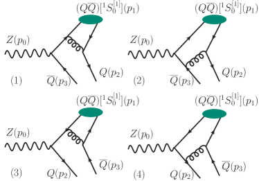
At the LO level, there are four Feynman diagrams for the decay process , which are shown in Fig.1. Corresponding to the four Feynman diagrams, the LO amplitude for this process can be written as , where
| (2) | |||||
| (3) | |||||
| (4) | |||||
| (5) | |||||
Here, and are vector and axial electroweak couplings, respectively. More explicitly, , , and . is the projector for -wave spin-singlet state
| (6) |
and is the color projector for color-singlet state
| (7) |
where 1 is the unit matrix of the group.
With these amplitudes, the LO decay width for the pair can be calculated through
| (8) |
where denotes the sum over the spin and color states of initial and final particles. is the differential phase space for the three-body final state, and
| (9) |
where is the number of the space-time dimensions. With these formulas, the LO decay width for can be calculated directly.
III NLO corrections
At the NLO level, the virtual and real corrections need to be calculated. There are ultraviolet (UV) and infrared (IR) divergences in virtual correction, and IR divergence in real correction. The conventional dimensional regularization with is employed to regularize both UV and IR divergences throughout this paper. In dimensional regularization, the problem is notorious, and we adopt a practical prescription proposed in Ref.Korner:1991sx . In the following subsections, we explain our main steps in calculating the virtual and real corrections.
III.1 Virtual NLO correction
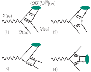
The virtual correction at the NLO level comes from the interference of the one-loop Feynman diagrams and the LO Feynman diagrams. Four typical one-loop Feynman diagrams are shown in Fig.2. It is noted that, compared to the case JXWang , there are new type Feynman diagrams, in which the pair is produced from two virtual gluons, need to be calculated in the case. These new type Feynman diagrams do not contribute to the case. One of the new type diagrams is shown by the fourth diagram in Fig.2.
The virtual correction to the decay width of the process can be calculated through
| (10) |
where is the amplitude for the virtual correction, and is the differential three-body phase space, which has been presented in Eq.(9).
In order to take the lowest-order nonrelativistic approximation, we need to expand the amplitude in (the relative momentum between the quark and antiquark in the pair). In the actual calculation, we expand the amplitude in (it is equivalent to taking here) before performing the loop integration. In the language of method of region region , this amounts to directly calculating the contributions from the hard region. The Coulomb divergence, which is power IR divergence, will vanish in the calculation under dimensional regularization.
There are UV and IR divergences in the loop integrals. The IR divergences from the virtual correction will be canceled by the IR divergences from the real correction. The UV divergences need to be removed through renormalization. The renormalization scheme is taken as follows: For the renormalization of the heavy quark field, the heavy quark mass and the gluon field, the on-mass-shell (OS) scheme is adopted, while for the renormalization of the strong coupling constant, the modified minimal subtraction () scheme is adopted. With this renormalization scheme, the quantities can be derived Klasen:2004tz
| (11) |
where is the renormalization scale, is the Euler constant. is the one-loop coefficient of the QCD function, in which is the number of active quark flavors. and is the number of light-quark flavors. When , we consider the charm-quark loop in the gluon self-energy but neglect the bottom-quark and top-quark loops in the gluon self-energy, i.e. ; when , we consider the charm-quark and bottom-quark loops in the gluon self-energy but neglect the top-quark loop in the gluon self-energy, i.e. . For group, , and .
In the calculations, the package FeynArts feynarts is employed to generate Feynman diagrams and amplitudes, the package FeynCalc feyncalc1 ; feyncalc2 is employed to carry out the color and Dirac traces, the packages $Apart apart and FIRE fire are employed to conduct partial fraction and integration-by-parts (IBP) reduction. After the IBP reduction, all one-loop integrals are reduced into master integrals, and the master integrals are calculated by the package LoopTools looptools numerically. The final phase-space integrations are calculated with the help of the package Vegas vegas .
III.2 Real NLO correction
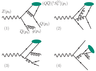
The real correction to the process comes from the process . Four typical Feynman diagrams are shown in Fig.3. Compared to the case, we need to deal with new type Feynman diagrams, in which the pair is produced from the gluon fragmentation, such as the fourth diagram of Fig.3.
Using these Feynman diagrams, the amplitude () for the real correction can be written down directly. Then the differential decay width for the real correction can be calculated through
| (12) |
where is the differential four-body phase space,
| (13) |
There are IR divergences in the real correction, which come from the phase-space integration over the region where the momentum of the final gluon is close to zero. We employ the two-cutoff phase-space slicing method twocutoff to isolate the IR divergences in the real correction. Due to the fact that there is no collinear divergence in the present process, we only need to introduce one cutoff parameter . Then the phase space for the real correction is divided into two regions: The soft region with and the hard region with . Here, we define the gluon energy in the rest frame of the initial boson. More explicitly, the real correction can be divided into two parts
| (14) |
where
| (15) |
and
| (16) |
Applying the eikonal approximation to the amplitude in the soft region twocutoff ; Bassetto:1983mvz , we obtain
| (17) |
Up to corrections, the differential phase space for the soft region can be factorized as twocutoff
| (18) |
where denotes the differential three-body phase space without emitting a gluon, whose expression has been shown in Eq.(9).
Inserting Eqs.(17) and (18) into Eq.(15), and carrying out the integration over Denner:1991kt ; Beenakker:2002nc , we obtain
where
where and are also defined in the rest frame of the initial boson.
Due to the constraint for the hard region, the contribution from the hard region is finite, then can be numerically calculated in four dimensions. The real correction can be obtained by summing the contributions from the hard and soft regions easily. Both the contributions from the soft and hard regions are separately dependent on the cutoff parameter , while the sum of these two contributions should be independent to the choice of ( should be small enough.). Verifying this independence is an important test of the correctness of the calculation. We have checked the independence, and have found that the results are independent of within the error of the numerical integration when varies from to .
The net NLO corrections can be obtained through summing the virtual and real corrections. After summing the virtual and real corrections, the UV and IR divergences are exactly canceled, and the finite results are obtained. The decay width can be obtained from by multiplying a factor , where is radial wave function at the origin, which can be calculated by using the potential model pot .
IV Numerical results and discussions
The input parameters for the numerical calculation are taken as follows Workman:2022ynf :
| (20) |
where and are the pole masses, is the electromagnetic coupling constant at . For the running strong coupling constant, we use the two-loop formula
| (21) |
where is the two-loop coefficient of the QCD function. According to Workman:2022ynf , we obtain and . With the values for , the strong coupling constant at any scale can be directly calculated through Eq.(21). For the radial wave functions at the origin, we adopt the values from the potential-model calculation pot , i.e.,
| (22) |
IV.1 Integrated decay widths
In this subsection, we give the integrated decay widths for the decay channel up to the NLO level.
| 0.245 | 62.7 | 84.3 | 1.34 | |
| 0.118 | 14.5 | 30.8 | 2.12 |
| 0.180 | 10.8 | 13.8 | 1.28 | |
| 0.118 | 4.65 | 8.49 | 1.83 |
In order to have a glance on the size of the NLO corrections, we first present the decay widths when the input quark masses are taken as their central values (i.e., and ), an analysis of the uncertainties of these decay widths will be presented later. The decay widths of up to the NLO level are given in Tables 1 and 2, where denotes the sum of the LO contribution and the NLO corrections. The renormalization scales are set as two energy scales involved in the processes, i.e., and . Tables 1 and 2 show that the NLO corrections contribute significantly to the decay widths in both cases. The NLO corrections increase the decay width of by for and for ; and they increase the decay width of by for and for .
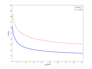
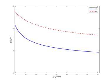
In Figs.4 and 5, the dependence of the decay widths on the renormalization scale is shown. After including the NLO corrections, the dependence of the decay widths on the renormalization scale is weakened. For , the decay width decreases by () at LO, and by () at NLO when varies from to . However, this dependence is still strong even including the NLO corrections.
Now, let us estimate the theoretical uncertainties for these decay widths. The main uncertainty sources include the renormalization scale, the heavy quark masses and the radial wave functions at the origin 444The Monte Carlo numerical integration in the calculation would lead to an error. However, the error of the numerical integration is on the order of for the case, and for the case in our calculation. Thus, the error from the numerical integration is negligible.. For the uncertainties caused by the renormalization scale, we estimate them by varying the renormalization scale between two physical energy scales involved in the processes, i.e. and . Furthermore, we take the average values of the decay widths under the two choices of the renormalization scale as their central values. For the uncertainties caused by the heavy quark masses, we estimate them by varying the heavy quark masses in the ranges given in Eq.(20), i.e., and . For the radial wave functions at the origin, the authors of Ref.pot did not give an error estimate. Since the potential used in Ref.pot does not include the spin effect, the wave functions calculated in this way are accurate up to corrections of relative order . Therefore, we estimate the uncertainties by attaching an error of of the central value for , and of the central value for . More explicitly, we take and . Then we obtain
| (23) |
and
| (24) |
Here, the first error is caused by the renormalization scale, the second error is caused by the heavy quark mass, and the last error is caused by the radial wave function at the origin. From Eqs.(23) and (24), we can see that the largest error arises from the renormalization scale uncertainty for both and cases. Furthermore, we find that although the K factors are sensitive to the renormalization scale, they are insensitive to the heavy quark mass, e.g., when we vary the charm (bottom) quark mass from () to (), the K factor changes from () to () for the () case.
Adding the uncertainties in quadrature, we obtain
| (25) |
and
| (26) |
IV.2 Differential decay widths
The differential distributions contain more information than the integrated decay widths, which can be used to test the current theory. Therefore, it is interesting to see the differential distributions of the two boson decay processes.
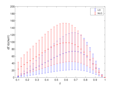
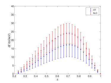
The energy fraction carrying by or in the processes can be defined as . The LO and NLO differential decay widths for the processes and are shown in Figs. 6 and 7, respectively. Figs. 6 and 7 confirm the importance of the NLO corrections. For the production, the magnitude of is increased obviously at small and moderate values and decreased slightly at higher values. And for the production, the magnitude of is increased at all values. The uncertainties for are also shown in the figures, which are obtained by combining the uncertainties of the renormalization scale, the heavy quark mass and the wave function at the origin.
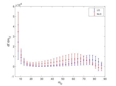
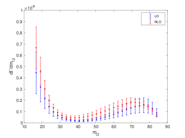
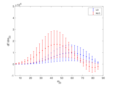
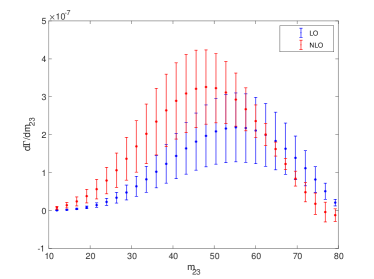
The momenta of heavy quarks in the final state can be determined experimentally using the heavy-flavor tagging technology. Therefore, the differential decay widths and can be measured experimentally, where and are invariant masses of two final-state particles. We present the LO and NLO differential decay widths and for and in Figs. 8, 9, 10 and 11, respectively. The uncertainties for these differential decay widths are also shown in these figures. From the figures, we can see that the differential decay widths and are changed significantly after including the NLO corrections, especially for the decay . Moreover, it is found that the NLO differential decay widths and are negative at the large or for . This indicates that the NLO corrections are negative and larger than LO contribution in these phase space regions. In the boundary regions of the phase space, some large logarithmic terms often appear in the coefficients of the perturbation expansion, which may spoil the convergence of the perturbation series. In these boundary regions, it is necessary to resum these large logarithmic terms so as to obtain precise theoretical results. Because of these large logarithmic terms, if we calculate to a certain order (e.g. NLO) in these regions, we may obtain nonphysical negative results. Fortunately, in the considered processes, the absolute values of the negative contributions of these regions are not large. Thus, we believe that the differential decay widths for most regions of the phase space and the integrated decay widths, which are obtained in this paper, are reliable.
V Summary
In the present paper, we have studied the decays and up to NLO QCD accuracy. Integrated and differential decay widths of both decay processes are obtained, and the uncertainties for them are estimated. We find that the NLO corrections to the decay widths for and are significant. The dependence of the decay widths on the renormalization scale is very strong although the dependence is weakened after including the NLO corrections. This brings a big uncertainty to the theoretical predictions under the conventional renormalization scale setting. The higher-order corrections can reduce the uncertainty caused by the renormalization scale. However, it is very difficult to calculate the higher-order corrections beyond the NLO for these processes at present. In the literature, the principle of maximum conformality (PMC) scale-setting approach pmc1 ; pmc2 ; pmc4 ; pmc5 has been suggested to eliminate such scale uncertainty, whose key idea is to determine the correct momentum flow of the process by using the nonconformal -terms that govern the running behavior with the help of renormalization group equation. As a comparison, we also calculate the integrated decay widths under the PMC scale setting. Following the standard PMC procedures to the decay width of , we obtain and . Here, the PMC predictions of the decay width are independent to the choices of , and the errors come from the uncertainties of the heavy quark masses and the wave functions at the origin.
The cross sections for at the pole 555The -exchange contribution is negligibly small at the pole, which can be safely neglected. can be derived from the decay widths through the formulas derived in the Appendix A1 of Ref.Zheng:2017xgj , i.e.,
| (27) | |||||
Then we obtain
| (28) | |||||
| (29) |
If the luminosity of a factory can be up to zfactory , there are about events and events to be produced per operation year. Moreover, the background of the Z factory is clean. Therefore, the two production processes may be studied at a high luminosity factory.
Acknowledgments: This work was supported in part by the Natural Science Foundation of China under Grants No. 12005028, No. 12175025, No. 12147116 and No. 12147102, by the China Postdoctoral Science Foundation under Grant No. 2021M693743, by the Fundamental Research Funds for the Central Universities under Grant No. 2020CQJQY-Z003, and by the Chongqing Graduate Research and Innovation Foundation under Grant No. ydstd1912.
References
- (1) H. Fritzsch, Producing Heavy Quark Flavors in Hadronic Collisions: A Test of Quantum Chromodynamics, Phys. Lett. B 67, 217-221 (1977).
- (2) F. Halzen, Cvc for Gluons and Hadroproduction of Quark Flavors, Phys. Lett. B 69, 105-108 (1977).
- (3) C. H. Chang, Hadronic Production of Associated With a Gluon, Nucl. Phys. B 172, 425-434 (1980).
- (4) E. L. Berger and D. L. Jones, Inelastic Photoproduction of J/psi and Upsilon by Gluons, Phys. Rev. D 23, 1521-1530 (1981).
- (5) T. Matsui and H. Satz, Suppression by Quark-Gluon Plasma Formation, Phys. Lett. B 178, 416-422 (1986).
- (6) G.T. Bodwin, E. Braaten and G.P. Lepage, Rigorous QCD analysis of inclusive annihilation and production of heavy quarkonium, Phys. Rev. D 51, 1125 (1995) [Erratum-ibid. D 55, 5853 (1997)].
- (7) N. Brambilla, et al. Heavy quarkonium: progress, puzzles, and opportunities, Eur. Phys. J. C 71, 1534 (2011) and references therein.
- (8) A. Andronic, F. Arleo, R. Arnaldi, A. Beraudo, E. Bruna, D. Caffarri, Z. C. del Valle, J. G. Contreras, T. Dahms and A. Dainese, et al. Heavy-flavour and quarkonium production in the LHC era: from proton–proton to heavy-ion collisions, Eur. Phys. J. C 76, no.3, 107 (2016).
- (9) J. P. Lansberg, New Observables in Inclusive Production of Quarkonia, Phys. Rept. 889, 1-106 (2020).
- (10) A. P. Chen, Y. Q. Ma and H. Zhang, A short theoretical review of charmonium production, arXiv:2109.04028 [hep-ph].
- (11) R. Aaij et al. [LHCb Collabration], Measurement of the production cross-section in proton-proton collisions via the decay , Eur. Phys. J. C 75, 311 (2015).
- (12) M. Butenschoen, Z. G. He and B. A. Kniehl, production at the LHC challenges nonrelativistic-QCD factorization, Phys. Rev. Lett. 114, 092004 (2015).
- (13) H. Han, Y. Q. Ma, C. Meng, H. S. Shao and K. T. Chao, production at LHC and indications on the understanding of production, Phys. Rev. Lett. 114, 092005 (2015).
- (14) H. F. Zhang, Z. Sun, W. L. Sang and R. Li, Impact of hadroproduction data on charmonium production and polarization within NRQCD framework, Phys. Rev. Lett. 114, 092006 (2015).
- (15) P. Pakhlov et al. [Belle], Measurement of the cross section at GeV, Phys. Rev. D 79, 071101 (2009).
- (16) Y. J. Li, G. Z. Xu, P. P. Zhang, Y. J. Zhang and K. Y. Liu, Study of Color Octet Matrix Elements Through Production in Annihilation, Eur. Phys. J. C 77, 597 (2017).
- (17) B. Guberina, J. H. Kuhn, R. D. Peccei and R. Ruckl, Rare Decays of the , Nucl. Phys. B 174, 317-334 (1980).
- (18) W. Y. Keung, Off Resonance Production of Heavy Vector Quarkonium States in Annihilation, Phys. Rev. D 23, 2072 (1981).
- (19) K. J. Abraham, Bottonium production at LEP, Z. Phys. C 44, 467-469 (1989).
- (20) V. D. Barger, K. m. Cheung and W. Y. Keung, Z-boson decays to heavy quarkonium, Phys. Rev. D 41, 1541 (1990).
- (21) K. Hagiwara, A. D. Martin and W. J. Stirling, J / psi production from gluon jets at LEP, Phys. Lett. B 267, 527-531 (1991).
- (22) E. Braaten, K. m. Cheung and T. C. Yuan, decay into charmonium via charm quark fragmentation, Phys. Rev. D 48, 4230-4235 (1993).
- (23) S. Fleming, Electromagnetic production of quarkonium in decay, Phys. Rev. D 48, 1914-1916 (1993).
- (24) K. m. Cheung, W. Y. Keung and T. C. Yuan, Color octet quarkonium production at the pole, Phys. Rev. Lett. 76, 877-880 (1996).
- (25) P. L. Cho, Prompt upsilon and psi production at LEP, Phys. Lett. B 368, 171-178 (1996).
- (26) P. Ernstrom, L. Lonnblad and M. Vanttinen, Evolution effects in fragmentation into charmonium, Z. Phys. C 76, 515-521 (1997).
- (27) G. A. Schuler, Quarkonium production: Velocity scaling rules and long distance matrix elements, Int. J. Mod. Phys. A 12, 3951-3964 (1997).
- (28) R. Li and J. X. Wang, Next-to-leading-order QCD correction to inclusive production in decay, Phys. Rev. D 82, 054006 (2010).
- (29) Q. L. Liao, Y. Yu, Y. Deng, G. Y. Xie and G. C. Wang, Excited heavy quarkonium production via Z0 decays at a high luminosity collider, Phys. Rev. D 91, 114030 (2015).
- (30) T. C. Huang and F. Petriello, Rare exclusive decays of the Z-boson revisited, Phys. Rev. D 92, 014007 (2015).
- (31) A. K. Likhoded and A. V. Luchinsky, Double Charmonia Production in Exclusive Boson Decays, Mod. Phys. Lett. A 33, 1850078 (2018).
- (32) G. T. Bodwin, H. S. Chung, J. H. Ee and J. Lee, -boson decays to a vector quarkonium plus a photon, Phys. Rev. D 97, 016009 (2018).
- (33) Z. Sun and H. F. Zhang, Next-to-leading-order QCD corrections to the decay of boson into , Phys. Rev. D 99, 094009 (2019).
- (34) H. S. Chung, J. H. Ee, D. Kang, U. R. Kim, J. Lee and X. P. Wang, Pseudoscalar Quarkonium+gamma Production at NLL+NLO accuracy, JHEP 10, 162 (2019).
- (35) X. C. Zheng, C. H. Chang and X. G. Wu, NLO fragmentation functions of heavy quarks into heavy quarkonia, Phys. Rev. D 100, 014005 (2019).
- (36) Z. Sun, The studies on at the next-to-leading-order QCD accuracy, Eur. Phys. J. C 80, 311 (2020).
- (37) Z. Sun and H. F. Zhang, Comprehensive studies of inclusive production in Z boson decay, JHEP 06, 152 (2021).
- (38) X. C. Zheng, C. H. Chang, X. G. Wu, X. D. Huang and G. Y. Wang, Inclusive production of heavy quarkonium Q via Z boson decays within the framework of nonrelativistic QCD, Phys. Rev. D 104, 054044 (2021).
- (39) Z. Sun, X. Luo and Y. Z. Jiang, Impact of on the inclusive meson yield in Z-boson decay, Phys. Rev. D 106, 034001 (2022).
- (40) H. Baer, T. Barklow, K. Fujii, Y. Gao, A. Hoang, S. Kanemura, J. List, H. E. Logan, A. Nomerotski and M. Perelstein, et al. The International Linear Collider Technical Design Report - Volume 2: Physics, arXiv:1306.6352 [hep-ph].
- (41) A. Abada et al. [FCC], FCC Physics Opportunities: Future Circular Collider Conceptual Design Report Volume 1, Eur. Phys. J. C 79, no.6, 474 (2019).
- (42) J. B. Guimarães da Costa et al. [CEPC Study Group], CEPC Conceptual Design Report: Volume 2 - Physics & Detector, arXiv:1811.10545 [hep-ex].
- (43) J. P. Ma and Z. X. Zhang (The super Z-factory group), Preface, Sci. China: Phys., Mech. Astron. 53, 1947 (2010).
- (44) J. Erler, S. Heinemeyer, W. Hollik, G. Weiglein and P. M. Zerwas, Physics impact of GigaZ, Phys. Lett. B 486, 125-133 (2000).
- (45) W. Buchmuller and S. H. H. Tye, Quarkonia and Quantum Chromodynamics, Phys. Rev. D 24, 132 (1981).
- (46) X. C. Zheng, Z. Y. Zhang and X. G. Wu, Fragmentation functions for a quark into a spin-singlet quarkonium: Different flavor case, Phys. Rev. D 103, no.7, 074004 (2021).
- (47) J. G. Korner, D. Kreimer and K. Schilcher, A Practicable gamma(5) scheme in dimensional regularization, Z. Phys. C 54, 503-512 (1992).
- (48) M. Beneke and V.A. Smirnov, Asymptotic expansion of Feynman integrals near threshold, Nucl. Phys. B522, 321 (1998).
- (49) M. Klasen, B. A. Kniehl, L. N. Mihaila and M. Steinhauser, plus jet associated production in two-photon collisions at next-to-leading order, Nucl. Phys. B 713, 487-521 (2005).
- (50) T. Hahn, Generating Feynman diagrams and amplitudes with FeynArts 3, Comput. Phys. Commun 140, 418 (2001).
- (51) R. Mertig, M. Bohm and A. Denner, Feyn Calc - Computer-algebraic calculation of Feynman amplitudes, Comput. Phys. Commun 64, 345 (1991).
- (52) V. Shtabovenko, R. Mertig and F. Orellana, New Developments in FeynCalc 9.0, Comput. Phys. Commun 207, 432 (2016).
- (53) F. Feng, $Apart: A Generalized Mathematica Apart Function, Comput. Phys. Commun 183, 2158 (2012).
- (54) A.V. Smirnov, Algorithm FIRE - Feynman Integral REduction, J. High Energy Phys. 0810, 107 (2008).
- (55) T. Hahn and M. Perez-Victoria, Automatized one loop calculations in four-dimensions and D-dimensions, Comput. Phys. Commun 118, 153 (1999).
- (56) G. P. Lepage, A new algorithm for adaptive multidimensional integration, J. Comp. Phys. 27, 192 (1978).
- (57) B.W. Harris and J.F. Owens, The Two cutoff phase space slicing method, Phys. Rev. D 65, 094032 (2001).
- (58) A. Bassetto, M. Ciafaloni and G. Marchesini, Jet Structure and Infrared Sensitive Quantities in Perturbative QCD, Phys. Rept. 100, 201-272 (1983).
- (59) A. Denner, Techniques for calculation of electroweak radiative corrections at the one loop level and results for W physics at LEP-200, Fortsch. Phys. 41, 307-420 (1993).
- (60) W. Beenakker, S. Dittmaier, M. Kramer, B. Plumper, M. Spira and P. M. Zerwas, NLO QCD corrections to t anti-t H production in hadron collisions, Nucl. Phys. B 653, 151-203 (2003).
- (61) E.J. Eichten and C. Quigg, Mesons with beauty and charm: Spectroscopy, Phys.Rev. D49, 5845 (1994).
- (62) R. L. Workman [Particle Data Group], Review of Particle Physics, PTEP 2022, 083C01 (2022).
- (63) S. J. Brodsky and X.-G. Wu, Scale Setting Using the Extended Renormalization Group and the Principle of Maximum Conformality: the QCD Coupling Constant at Four Loops, Phys. Rev. D 85, 034038 (2012).
- (64) S. J. Brodsky and X.-G. Wu, Eliminating the Renormalization Scale Ambiguity for Top-Pair Production Using the Principle of Maximum Conformality, Phys. Rev. Lett. 109, 042002 (2012).
- (65) M. Mojaza, S. J. Brodsky, and X.-G. Wu, Systematic All-Orders Method to Eliminate Renormalization-Scale and Scheme Ambiguities in Perturbative QCD, Phys. Rev. Lett. 110, 192001 (2013).
- (66) S. J. Brodsky, M. Mojaza, and X.-G. Wu, Systematic Scale-Setting to All Orders: The Principle of Maximum Conformality and Commensurate Scale Relations, Phys. Rev. D 89, 014027 (2014).
- (67) X. C. Zheng, C. H. Chang, T. F. Feng and Z. Pan, NLO QCD corrections to Bc(B*c) production around the Z pole at an e+ e- collider, Sci. China Phys. Mech. Astron. 61, 031012 (2018).