New Results in Sona Drawing: Hardness and TSP Separation
Abstract
Given a set of point sites, a sona drawing is a single closed curve, disjoint from the sites and intersecting itself only in simple crossings, so that each bounded region of its complement contains exactly one of the sites. We prove that it is NP-hard to find a minimum-length sona drawing for given points, and that such a curve can be longer than the TSP tour of the same points by a factor . When restricted to tours that lie on the edges of a square grid, with points in the grid cells, we prove that it is NP-hard even to decide whether such a tour exists. These results answer questions posed at CCCG 2006.
In memoriam Godfried Toussaint (1944–2019)
1 Introduction
In April 2005, Godfried Toussaint visited the second author at MIT, where he proposed a computational geometric analysis of the “sona” sand drawings of the Tshokwe people in the West Central Bantu area of Africa. Godfried encountered sona drawings, in particular the ethnomathematical work of Ascher [1] and Gerdes [7], during his research into African rhythms. Together with his then-student Perouz Taslakian, we came up with a formal model of sona drawing of a set of point sites — a closed curve drawn in the plane such that
-
1.
wherever the curve touches itself, it crosses itself;
-
2.
each crossing involves only two arcs of the curve;
-
3.
exactly one site is in each bounded face formed by the curve; and
-
4.
no sites lie on the curve or within its outside face.
Our first paper on sona drawings appeared at BRIDGES 2006 [5], detailing the related cultural practices, proving and computing combinatorial results and drawings, and posing several open problems. In early 2006, we brought these open problems to Godfried’s Bellairs Winter Workshop on Computational Geometry, where a much larger group tackled sona drawings, resulting in a CCCG 2006 paper later the same year [4]. Next we highlight some of the key prior results and open problems as they relate to the results of this paper.
Sona vs. TSP.
Every TSP tour can be easily converted into a sona drawing of roughly the same length: instead of visiting a site, loop around it, except for one site that we place slightly interior to the tour [5, Lemma 11]. Conversely, every sona drawing can be converted into a TSP tour of length at most a factor larger [4, Theorem 12], settling [5, Open Problem 6]. Is this constant tight? The best previous lower bound was a four-site example proving a TSP/sona separation factor of [5, Lemma 12]. In Section 2, we construct a recursive family of examples proving a much larger TSP/sona separation factor of . We also study and metrics, where we prove that the worst-case TSP/sona separation factor is exactly .
Length minimization.
Grid drawings.
The last variant we consider is when the sona drawing is restricted to lie along the edges of a unit-square grid, while sites are at the centers of cells of the grid. Not all point sets admit a grid sona drawing; however, if we scale the sites’ coordinates by a factor of , then they always do [4, Proposition 10]. A natural remaining question [4, Open Problem 3] is which point sets admit grid sona drawings. In Section 4, we prove that this question is in fact NP-hard.
2 Separation from TSP Tour
We first show an example which gives a large TSP/sona separation factor under the metric in the plane.
Theorem 2.1.
There exists a set of sites for which the length of the minimum-length TSP tour is times the length of the minimum-length sona drawing.


The full proof can be found in Appendix A.
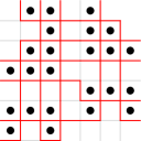
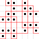
Sketch of Proof. We construct a problem instance whose minimum-length TSP tour is longer than its minimum-length sona drawing by a factor within of . Our construction is illustrated in Figure 1 and follows a fractal approach with levels (for simplicity, we assume that is an integer).
-
1.
We start by defining a few auxiliary points:
-
(a)
The initial set of auxiliary points is the intersection between a slightly shifted integer lattice and the ball of radius centered at the origin. That is, . In Figure 1(a), the auxiliary points are exactly the intersections of solid red lines.
-
(b)
Then, in Step (starting with ), for each auxiliary point , we add five points to : itself, and four new points at distance from in each of the four cardinal directions. Let . By construction, we have and . We note that set contains auxiliary points (not sites). These points will not be part of the instance.
-
(a)
-
2.
We now use the auxiliary points to create some sites (the isolated black points of Figure 1):
-
(a)
For any we define set of sites as follows: for each auxiliary point we add the four sites whose and coordinates each differ from by . We note that all the added sites are distinct sites.
-
(b)
We define as the set of integer lattice points in . Equivalently, for each auxiliary point we add the sites whose and coordinates each differ from by , but we do not add sites that lie outside , which affects sites (out of sites of ).
In this case, the sites created by different auxiliary points may lie in the same spot. In total, contains only one site per auxiliary point of (except for auxiliary points near the boundary). Thus, (for ) and .
Let .
-
(a)
-
3.
Next, we place additional sona sites packing line segments and/or curves. Whenever we pack any curve, we place sites spaced at a distance small enough that the length of the shortest path that passes within of all of them is within a factor of the length of the curve.
-
(a)
Solid lines as drawn in red in Figure 1(a): for each , we pack the vertical line segment with endpoints and , and analogously with for the horizontal line segments.
-
(b)
In Step of the above recursive definition (starting with ), when we create four new auxiliary points of from a point , we also pack the boundary of the region within Euclidean distance of the square whose vertices are the four auxiliary points of . Note that this boundary region forms a square with rounded corners as in Figure 1(b). With these extra points we preserve the invariant that the auxiliary points are exactly the intersections of packed curves.
-
(a)
Let be the set of sites created in Step 3 in our construction, and . This is a complete description of the construction.
In the full proof we show that the length of the packed curves is a -approximation of the total length of the minimum-length sona drawing of . Careful calculations then yield that the length of the minimum-length sona drawing is We then argue that the minimum-length TSP has an additional length of . Thus, the TSP/sona separation factor for the construction is, ignoring lower-order terms, .
We have presented a construction for the metric in the plane showing that the ratio between the lengths of the minimum-length TSP and the minimum-length sona drawing can be strictly greater than 1.5. Our next result shows that this cannot be the case for the and metrics in the plane.
Theorem 2.2.
For the Manhattan () and the Chebyshev () metrics, the minimum-length TSP tour for a set of sites has length at most times that of the minimum-length sona drawing for . Moreover, this bound is tight for both metrics.
Proof 2.3.
The proof of the upper bound on the length of the minimum-length TSP tour follows the lines of the (unpublished) proof of [4, Theorem 12]. Let be a set of sites, the minimum-length sona drawing for , and the minimum-length TSP tour for . The sona drawing must have bounded faces, each containing a site of . Let be the face of containing the site . In this proof, for an edge-weighted graph , denotes the sum of the weights/lengths of all the edges of . In particular, denotes the length of the sona drawing .
For each site , let be the closest point in to and the distance between and . By the definition of , the open disk centered at and with radius does not intersect . This implies that the length of the boundary of is at least the perimeter of a disk with radius , that for both the and the metrics is . That is, . Moreover, the sum of the lengths of all the faces is , so since we do not sum the length of the unbounded face.
We define a multigraph whose vertex set is the union of the set of sites , the set of vertices of , and . The edge set of is the union of the set of edges of and two parallel edges for each . The weight of each edge is its length in the drawing. By the observations above, .
To obtain the desired upper bound on it remains to show that . By construction, since is Eulerian, so is . An Euler tour of defines a TSP tour for the vertices of by skipping vertices that were already visited (as in the Christofides 1.5-approximation algorithm for TSP on instances where the distances form a metric space [3]). This TSP tour has length at most and can be shortcut so that it only visits the sites of . By the triangle inequality, the length of the tour does not increase with these shortcuts. Thus, we have that .
The construction for the matching this bound is similar to the one in the proof of Theorem 2.1, but simpler. An illustration can be found in Figure 1(a). For every we construct a set of sites (the set of TSP vertices/sona sites) such that .
We fix . The set of sites includes every integer lattice point such that . Consider drawing resulting from the union of the axis-aligned unit squares centered at these sites. It is easy to see, for example by rotating the construction, that so far we have added sites to and that the length of is . Straightforward computations show that . Thus, a dense-enough packing of sites along yields the desired result.
We next consider sona drawings on the sphere. By the definition of sona drawings in the plane, the unbounded face contains no sites. For the sphere we consider the following analogue: if there is a face that contains in its interior a half-sphere then this face contains no sites. Note that there is at most one such face. The following theorem shows a tight upper bound on the TSP/sona separation factor for drawings on the sphere. (We consider the usual metric inherited from the Euclidean metric in .)
Theorem 2.4.
For drawings on the sphere, the length of the minimum-length TSP tour for a set of sites is at most times the length of the minimum-length sona drawing for . Moreover, this bound is tight.
Proof 2.5.
The proof of the upper bound on the length of the minimum-length TSP tour again follows the lines of the (unpublished) proof of [4, Theorem 12]. It only differs slightly from the first part of the the proof of Theorem 2.2. Using the same notation, in this case, the distance between a site and its closest point in corresponds to the length of the shortest arc on the great circle through and . The open disk centered at and with radius is an open spherical cap that does not intersect . Assuming that the sphere has radius , the boundary of this cap has length . Since the face containing a site cannot contain a half-sphere in its interior we have that . The function in the interval is decreasing. Thus, . This implies that . Thus, the face of containing the site has length . Moreover, . With the same arguments and defining the same multigraph as in the proof of Theorem 2.2 we obtain that .
The construction showing that this bound is tight places two sites on the north and south poles of the sphere and packs the equator densely with sites. Then the minimum-length sona drawing goes along the equator while the minimum-length TSP must reach both poles, yielding a TSP/sona separation factor.
3 Complexity of Length Minimization
In this section and Appendix B, we prove that finding a sona drawing of minimum length for given sites is NP-hard, even when the sites lie on a polynomially sized grid. The complexity of minimum-length sona drawing was posed as an open problem in 2006 by Damian et al. [4, Open Problem 4]. We use a reduction from the problem of finding a Hamiltonian cycle in a grid graph (a graph whose vertices are a subset of the points in an integer grid, and whose edges are the unit-length line segments between pairs of vertices), proven NP-complete by Itai, Papadimitriou, and Szwarcfiter [8].
Let be the set of vertices in a hard instance for Hamiltonian cycle in grid graphs. If is a yes instance, its Hamiltonian cycle forms a Euclidean traveling salesman tour with length exactly . If it is a no instance, the shortest Euclidean traveling salesman tour through its vertices has length at least for every grid edge, and length at least for at least one edge that is not a grid edge (as this is the shortest distance between grid points that are non-adjacent), so its total length is at least . For the distance, the increase in length is larger, at least . Our reduction replaces each point of by two points, close enough together to make the increase in length from converting a TSP to a sona drawing negligible with respect to this gap in tour length.
Theorem 3.1.
It is NP-hard to find a sona drawing for a given set of sites whose length is less than a given threshold , for any of the , , and metrics.
4 Complexity of Grid Drawing Existence
While minimizing the length of sona drawings in general is hard, if we restrict the drawing to lie on a grid, then even determining the existence of a sona drawing is hard.
Given sites at the centers of some cells in the unit-square grid, a grid sona drawing is a sona drawing whose edges are drawn as polygonal lines along the orthogonal grid lines (like orthogonal graph drawing).
We show that finding a grid sona drawing for a given set of sites is NP-hard by a reduction from Planar CNF SAT [9].
4.1 Construction
In this section we view the grid as a graph, thus by edge we mean a unit segment of a grid line, and by vertex we mean a grid vertex — these terms are distinct from “sona edge” etc. We say that an edge is either on or off according to as it belongs in the sona drawing. The subgraph of the grid that is on is the path graph. Observe that two grid-adjacent sites always require the edge between them to be on; otherwise both would be in the same sona face (connected). Also, every vertex must have even degree in the path graph.
Here we are concerned with internal properties of the gadgets. Their exteriors are lined with unconnected edges; we will show later how to connect them.


Wire.
The wire gadget is shown in Figure 4. One of edges and must be on, otherwise two sites would be connected. Assume without loss of generality that is on. Now, suppose is off. Then must be too, to preserve even vertex degree. Then, and must both be on to prevent sites from being connected, but this is impossible with off. Therefore and are on. The same reasoning shows that the entire line , , etc. is on, as well as edges , , etc. Then must be off to prevent an empty face, and thus the entire line , , etc. is off. The wire thus has two states: the upper line can be on and the lower off, or vice-versa. We can extend a wire as long as necessary. An unconnected wire end serves as a variable.
Constant.
The gadget shown in Figure 4 forces the attached wire to be in the up state: the edge between the two left sites must be on, forcing the rest.
Turn / Split / Invert.
The gadget shown in Figure 4 is multi-purpose. If we view the left wire as the input, then the upper and lower outputs represent turned signals, and the right output represents an inverted signal. (Unused outputs can be left unattached, thus unconstrained.)
Any wire state forces all the others. Given that the left wire is in the up state, suppose the right wire is also up. Then the top wire and bottom wire must be in the same left/right state, otherwise we will have degree-three vertices in the middle. But this would leave the central site connected to another site, so the right wire is forced down. Then, if the (top, bottom) wires are not in the (left, right) states, again the central site will be connected to another one. (This figure contains multiple loops, but these will be eliminated in the final configuration by adding more edges.)


OR.
Figure 5 shows the OR gadget. The upper wire is interpreted as an output, with the left state representing true; the other wires are inputs, with true represented as down on the left wire and up on the right wire. (We can easily adjust truth representations between gadgets with inverters.) If either input is true, then the output may be set true, as shown. If both inputs are false, the output may be set false. 5(e) shows that setting the output to true when both inputs are false is not possible: all marked edge states are forced by the wire properties, but two sites are left connected.
4.2 Hardness
Theorem 4.1.
It is NP-hard to find a grid sona drawing for a given set of sites at the centers of grid cells.
Proof 4.2.
Given a CNF Boolean formula with a planar incidence graph, we connect the above gadgets to represent this graph: unconstrained wire ends represent variables, and are connected to splitters and inverters to reach clause constructions. A clause is implemented with chained OR gadgets, with the final output constrained to be true with a constant gadget. By the gadget properties described above, we will be able to consistently choose wire states if and only if the formula is satisfiable.
We must still show that all edges can be joined together into a single closed loop, while retaining the sona properties. Our basic strategy for connecting loose ends is to border each gadget with “crenellations”, as shown in Figure 6. This figure also shows how to pass pairs of path segments across a wire without affecting its internal properties, which we will use to help form a single loop.


Adding crenellations to the other gadgets is straightforward, and we defer explicit figures to Appendix C, with one exception. (The crenellations do add a parity constraint when wiring gadgets together; we show in the appendix how to shift parity.) When we use the gadget in Figure 4 to turn a wire, it will be useful to use the crenellated version in Figure 7. With the connections to other gadgets on the left and top, the right and bottom portions are unconstrained. We can place edges as shown, so that they leave the gadget identically regardless of which state it is in. Then, all paths entering from the left or the top leave on the bottom or the right as loose edges, except that in 7(a), one path connects the left to the top. If we connect a right turn to the top port, this path will also terminate in an unconnected edge. If every wire contains a left turn and matching right turn, then every path in the sona graph must end in two unconnected edges in turn gadgets, because there are no internal loops in any of the gadgets.
The space occupied by the loose ends of a turn lies either in an internal face of the wiring graph, or on its exterior. We route the interior ends to pass-through pairs as shown in Figure 6, so all unconnected edges wind up on the outer border of the graph. Because the terminal edges are placed identically in Figures 7(a) and 7(b), we can plan their routing without knowing the wire states. As a result, we can place additional sites as required for the property that a single site lies in each internal sona face. (We can lengthen the wires as needed to create additional routing space in the internal faces.)
Now we are in a state where all paths end on the exterior of the construction. If we join these paths together without crossing, the number of extra sites needed in the outer face is just the number of paths. We place that many sites in a widely spaced grid (spacing proportional to number of paths) surrounding the inner construction. Then, we can complete the path greedily by repeatedly connecting one outer path end to one of its neighboring path ends, surrounding one of the added sites. Only one of its two neighboring path ends can come from the same path, so there’s always another one to connect to. The wide grid spacing of the outer sites means there is always room to route the connection.
Acknowledgments
Thanks to Godfried Toussaint for introducing us (and computational geometry) to sona drawings. This research was initiated during the Virtual Workshop on Computational Geometry held March 20–27, 2020, which would have been the 35th Bellairs Winter Workshop on Computational Geometry co-organized by E. Demaine and G. Toussaint if not for other circumstances. We thank the other participants of that workshop for helpful discussions and providing an inspiring atmosphere.
References
- [1] Marcia Ascher. Mathematics Elsewhere: An Exploration of Ideas Across Cultures. Princeton University Press, 2002.
- [2] Molly Baird, Sara C. Billey, Erik D. Demaine, Martin L. Demaine, David Eppstein, Sándor Fekete, Graham Gordon, Sean Griffin, Joseph S. B. Mitchell, and Joshua P. Swanson. Existence and hardness of conveyor belts. Electronic preprint arXiv:1908.07668, 2019. URL: https://arXiv.org/abs/1908.07668.
- [3] Nicos Christofides. Worst-case analysis of a new heuristic for the travelling salesman problem. Technical report, Graduate School of Industrial Administration, Carnegie Mellon University, 1976.
- [4] Mirela Damian, Erik D. Demaine, Martin L. Demaine, Vida Dujmović, Dania El-Khechen, Robin Flatland, John Iacono, Stefan Langerman, Henk Meijer, Suneeta Ramaswami, Diane L. Souvaine, Perouz Taslakian, and Godfried T. Toussaint. Curves in the sand: Algorithmic drawing. In Proceedings of the 18th Annual Canadian Conference on Computational Geometry (CCCG 2006), pages 11–14, Kingston, Ontario, August 2006. URL: https://cccg.ca/proceedings/2006/cccg4.pdf.
- [5] Erik D. Demaine, Martin L. Demaine, Perouz Taslakian, and Godfried T. Toussaint. Sand drawings and Gaussian graphs. Journal of Mathematics and The Arts, 1(2):125–132, June 2007. Originally at BRIDGES 2006. doi:10.1080/17513470701413451.
- [6] Erik D. Demaine, Joseph S. B. Mitchell, and Joseph O’Rourke. Problem 33: Sum of Square Roots. In The Open Problems Project. Smith College, September 19 2017. URL: https://cs.smith.edu/~jorourke/TOPP/P33.html.
- [7] Paulus Gerdes. The ‘sona’ sand drawing tradition and possibilities for its educational use. In Geometry From Africa: Mathematical and Educational Explorations, pages 156–205. The Mathematical Association of America, 1999.
- [8] Alon Itai, Christos H. Papadimitriou, and Jayme Luiz Szwarcfiter. Hamilton paths in grid graphs. SIAM Journal on Computing, 11(4):676–686, 1982. doi:10.1137/0211056.
- [9] David Lichtenstein. Planar formulae and their uses. SIAM Journal on Computing, 11(2):329–343, 1982. URL: https://doi.org/10.1137/0211025, doi:10.1137/0211025.
- [10] Joseph O’Rourke. Advanced problem 6369. American Mathematical Monthly, 88(10):769, 1981. doi:10.2307/2321488.
Appendix A Separation from TSP Tour under the Metric
Theorem 2.1.
There exists a set of sites for which the length of the minimum-length TSP tour is times the length of the minimum-length sona drawing.
Proof A.1.
We construct a problem instance whose minimum-length TSP tour is longer than its minimum-length sona drawing by a factor within of . Our construction is illustrated in Figure 1 and follows a fractal approach with levels (for simplicity, we assume that is an integer).
-
1.
We start by defining a few auxiliary points:
-
(a)
The initial set of auxiliary points is the intersection between a slightly shifted integer lattice and the ball of radius centered at the origin. That is, . In Figure 1(a), the auxiliary points are exactly the intersections of solid red lines.
-
(b)
Then, in Step (starting with ), for each auxiliary point , we add five points to : itself, and four new points at distance from in each of the four cardinal directions. Let . By construction, we have and . We note that set contains auxiliary points (not sites). These points will not be part of the instance.
-
(a)
-
2.
We now use the auxiliary points to create some sites (the isolated black points of Figure 1):
-
(a)
For any we define set of sites as follows: for each auxiliary point we add the four sites whose and coordinates each differ from by . We note that all the added sites are distinct sites.
-
(b)
We define as the set of integer lattice points in . Equivalently, for each auxiliary point we add the sites whose and coordinates each differ from by , but we do not add sites that lie outside , which affects sites (out of sites of ).
In this case, the sites created by different auxiliary points may lie in the same spot. In total, contains only one site per auxiliary point of (except for auxiliary points near the boundary). Thus, (for ) and .
Let .
-
(a)
-
3.
Next, we place additional sona sites packing line segments and/or curves. Whenever we pack any curve, we place sites spaced at a distance small enough that the length of the shortest path that passes within of all of them is within a factor of the length of the curve.
-
(a)
Solid lines as drawn in red in Figure 1(a): for each , we pack the vertical line segment with endpoints and , and analogously with for the horizontal line segments.
-
(b)
In Step of the above recursive definition (starting with ), when we create four new auxiliary points of from a point , we also pack the boundary of the region within Euclidean distance of the square whose vertices are the four auxiliary points of . Note that this boundary region forms a square with rounded corners as in Figure 1(b). With these extra points we preserve the invariant that the auxiliary points are exactly the intersections of packed curves.
-
(a)
Let be the set of sites created in Step 3 in our construction, and . This is a complete description of the construction.
We now find the minimum-length sona drawing of . Each pair of consecutive points in a packed curve must be in a separate sona region, so any sona drawing must pass between them; in particular, any sona drawing must pass within of each of them, and so the length of any valid sona drawing is at least times the length of the packed curves. Also, there’s a valid sona drawing that’s at most times the length of the packed curves: follow all the packed curves exactly, adding small loops around the sona sites of the packed curves as necessary (loops small enough to lengthen the curve by a factor of at most ). The graph of packed curves is Eulerian (because it’s defined as a union of boundaries of regions, which are cycles), so the TSP tour can follow an Eulerian circuit through it. At an intersection of packed curves, we have two options for the sona drawing (as shown in the inset images of Figure 1). We can have one sona path cross over the other in the Eulerian circuit (by including every site of the packed curve in a small loop). Alternatively, we can have one sona path cross over the other in two places and at the intersection, and leaving one sona site of the packed curve out of a small loop to be the sona site of the extra region between and . In either case, we conclude that there is a valid sona path that follows an Eulerian circuit of the packed curves within . Note that, although our description focused in the sites of , this is a valid sona tour for since the sites of lie in different faces.
The total length of the packed curves is hence a -approximation of the total length of the minimum-length sona drawing.
The total length of the packed segments of (the square lattice) is , since the area of the region and the number of lattice points in it are each .
Now we bound the length of the packed curves (rounded squares). In Step of the construction (starting with ), we added a packed curve that is the boundary of the region within Euclidean distance of a square of side length (with a total length of ).
Recall that we added one such curve for each of the points of and that . Thus, the total length of the sona drawings introduced at Step is .
For small, this series is well-approximated by an infinite geometric series with sum , and adding in the length of the packed segments of (the square lattice) gives
We have approximated the minimum length of a valid sona drawing; now we approximate the minimum length of a TSP tour.
Any TSP tour must also come within of every point on every packed curve, which requires a length at least as above. Also, the TSP tour must visit each site of . We observe some properties of this set:
-
•
Set is defined so that sites are far from each other. Specifically, the Euclidean ball centered at any site of radius does not contain other sona sites. This means that we must include at least in the length of the TSP tour for each point in , for the part of the tour that passes from the boundary of this ball to and then back to the boundary.
-
•
There are sites in (for ) and sites in .
When tends to zero, the additional length needed in the TSP tour is
So, the total length of the TSP tour is at least . Hence the ratio of the length of the TSP tour to the length of the sona drawing is, ignoring lower-order terms, .
Appendix B Complexity of Length Minimization
Theorem 3.1.
It is NP-hard to find a sona drawing for a given set of sites whose length is less than a given threshold , for any of the , , and metrics.
Proof B.1.
Let be the set of vertices in a hard instance for finding a Hamiltonian cycle in grid graphs. We may form a hard instance of the minimum-length sona drawing problem for or distances by replacing each vertex in by a pair of sites, one at the original vertex position and the other at distance less than from it, where is chosen to be small enough that . We set . For distance, we use a hard instance for distance, rotated by .

If is a yes-instance for Hamiltonian cycle, let be a Hamiltonian cycle of length for . We may form a sona drawing of length less than by modifying within a neighborhood of each pair of sites so that, for all but one of these pairs, it makes two loops, one surrounding each site (Figure 8), and so that for the remaining pair it makes one loop around one of the two sites and surrounds the other point by the face formed by itself. In this way, each face of the modified curve surrounds a single site of our instance. Each of these local modifications to may be performed using additional length less than , so the total length of the resulting sona drawing is less than .
If is a no instance for Hamiltonian cycle, let be any sona drawing for the resulting instance of the minimum-length sona drawing problem. Then must pass between each pair of sites in the instance, and by making a local modification of length at most near each pair, we can cause it to touch the point in the pair that belongs to itself. Thus, we have a curve of length touching all points of . Because is a no instance, the length of this curve must be at least , from which it follows that the length of is at least .
By scaling the sites by a factor of we may obtain a hard instance of the minimum-length sona drawing problem in which all sites lie in an integer grid whose bounding box has side length .
It is possible to represent a minimum-length sona drawing combinatorially, as a conveyor belt [2] formed by bitangents and arcs of infinitesimally small disks centered at each site, and to verify in polynomial time that a representation of this form is a valid sona drawing. However, this does not suffice to prove that the decision version of the minimum-length sona drawing problem belongs to NP. The reason is that, when the sites have integer coordinates, the limiting length of a sona drawing, represented combinatorially in this way, is a sum of square roots (distances between pairs of given points) and we do not know the computational complexity of testing inequalities involving sums of square roots [10, 6]. (Euclidean TSP has the same issue.)
Appendix C Crenellations for Grid Drawing
Figures 9, 10, and 11 show how to add crenellations to the Constant gadget, an unconstrained wire end (variable), and the OR gadget, respectively. The crenellated Split / Invert is the same as in Figure 7, extended in the obvious way for ports that are used. In no case do the crenellations affect the internal properties described in the main text; these figures simply show that it is possible to add the crenellations appropriately.
As mentioned in the main text, the crenellations do add a parity constraint when connecting gadgets with wires; we can no longer make wires of arbitrary length, but must match the crenellations to the gadgets at each end. In order to do that we need one additional gadget, an inverting turn, shown in Figure 12. Unlike in Figure 7, the wire state is switched during the turn. Observe that in Figure 7, turning does not change crenellation parity, but the straight-through path, which would invert if not terminated, does change crenellation parity. The inverting turn also does not change crenellation parity. Therefore, to change the crenellation parity of a wire, we can invert it (straight through), changing the parity, and add a sequence left inverting turn, right turn, right turn, left turn to restore the original line of the wire.