Anyang, Henan 455000, Chinabbinstitutetext: Institute of Particle Physics and Key Laboratory of Quark and Lepton Physics (MOE),
Central China Normal University, Wuhan, Hubei 430079, China
New physics in the angular distribution of decay
Abstract
In decay, the three-momentum cannot be determined accurately due to the decay products of inevitably include an undetected . As a consequence, the angular distribution of this decay cannot be measured. In this work, we construct a measurable angular distribution by considering the subsequent decay . The full cascade decay is , in which the three-momenta , , and can be measured. The five-fold differential angular distribution containing all Lorentz structures of the new physics (NP) effective operators can be written in terms of twelve angular observables . Integrating over the energy of pion , we construct twelve normalized angular observables and two lepton-flavor-universality ratios . Based on the form factors calculated by the latest lattice QCD and sum rule, we predict the distribution of all and both within the Standard Model and in eight NP benchmark points. We find that the benchmark BP2 (corresponding to the hypothesis of tensor operator) has the greatest effect on all and , except . The ratios are more sensitive to the NP with pseudo-scalar operators than the . Finally, we discuss the symmetries in the angular observables and present a model-independent method to determine the existence of tensor operators.
1 Introduction
Exploring new physics (NP) beyond the Standard Model (SM) has been one of the most important tasks in high energy physics, especially since the discovery of Higgs boson Aad:2012tfa ; Chatrchyan:2012ufa ; Aad:2015zhl . In recent years, the existence of NP that breaks the universality of lepton flavour in transition has been implied by the anomalous measurements Lees:2012xj ; Lees:2013uzd ; Aaij:2015yra ; Huschle:2015rga ; Hirose:2016wfn ; Aaij:2017uff ; Hirose:2017dxl ; Aaij:2017deq ; Belle:2019rba on decays. Moreover, the averaging results performed by the Heavy Flavor Averaging Group (HFLAV) Amhis:2019ckw show that the measurements of () deviate about Amhis:2019up from the predicted values within the SM.111The recent ref. Bordone:2019vic finds in the SM. Since the HFLAV average does not include this value, the actual deviation from the SM prediction is larger than . Very recently, the review Bernlochner:2021vlv revisits the world averages by investigating the correlations between the systematic uncertainties of all measurements, and shows that their averages lead to an increased tension of about with respect to the SM. Motivated by this deviation and using the available data on transition, a number of global fitting analyses have been carried out Alok:2017qsi ; Hu:2018veh ; Alok:2019uqc ; Murgui:2019czp ; Blanke:2018yud ; Blanke:2019qrx ; Shi:2019gxi ; Cheung:2020sbq ; Kumbhakar:2020jdz , finding that some different combinations of NP coupling parameters can well explain the anomaly. At the same time, a large number of works have been completed in some specific NP models, such as leptoquarks Tanaka:2012nw ; Sakaki:2013bfa ; Bauer:2015knc ; Fajfer:2015ycq ; Li:2016vvp ; Crivellin:2017zlb ; Becirevic:2018afm ; Angelescu:2018tyl ; Bansal:2018nwp ; Iguro:2018vqb ; Crivellin:2019dwb , -parity violating supersymetric models Deshpand:2016cpw ; Altmannshofer:2017poe ; Hu:2018lmk ; Hu:2020yvs ; Altmannshofer:2020axr , charged Higgses Tanaka:2012nw ; Crivellin:2012ye ; Celis:2012dk ; Ko:2012sv ; Celis:2016azn ; Iguro:2017ysu ; Iguro:2018qzf , charged vector bosons Asadi:2018wea ; Greljo:2018ogz ; Babu:2018vrl , and Pati-Salam Model Blanke:2018sro ; Iguro:2021kdw . These NP effects also affect other semileptonic decay modes, such as Aaij:2017tyk ; Harrison:2020nrv ; Harrison:2020gvo ; Watanabe:2017mip ; Wei:2018vmk ; Tran:2018kuv ; Issadykov:2018myx ; Cohen:2018vhw ; Cohen:2018dgz ; Huang:2018nnq ; Wang:2018duy ; Leljak:2019eyw ; Hu:2019qcn ; Azizi:2019aaf ; Penalva:2020ftd , Wei:2018vmk ; Tran:2018kuv ; Issadykov:2018myx ; Berns:2018vpl ; Murphy:2018sqg ; Wang:2018duy ; Leljak:2019eyw ; Hu:2019qcn ; Azizi:2019aaf ; Penalva:2020ftd , Dutta:2015ueb ; Li:2016pdv ; Hu:2018veh ; DiSalvo:2018ngq ; Ray:2018hrx ; Penalva:2019rgt ; Mu:2019bin ; Gutsche:2015mxa ; Shivashankara:2015cta ; Boer:2019zmp ; Ferrillo:2019owd ; Hu:2020axt , Dutta:2018zqp ; Faustov:2018ahb ; Zhang:2019jax ; Zhang:2019xdm , Rajeev:2019ktp ; Sheng:2020drc , and Rajeev:2019ktp ; Sheng:2020drc .
Particularly, the LHCb collaboration released a value of the ratio Aaij:2017tyk . Using the model-dependent calculations of transition form factors Kiselev:1999sc ; Ivanov:2000aj ; Ebert:2003cn ; Hernandez:2006gt ; Ivanov:2006ni ; Wang:2008xt ; Qiao:2012vt ; Wen-Fei:2013uea ; Rui:2016opu ; Dutta:2017xmj ; Watanabe:2017mip ; Tran:2018kuv ; Issadykov:2018myx ; Leljak:2019eyw ; Hu:2019qcn , the SM prediction of lies in the range 0.23–0.30. The model-independent bound on Cohen:2018dgz ; Wang:2018duy is also obtained by constraining the form factors through a combination of dispersive relations, heavy-quark relations at zero-recoil, and the limited existing form-factor determinations from lattice QCD Colquhoun:2016osw ; Lytle:2016ixw , resulting in Cohen:2018dgz . Very recently, the HPQCD collaboration present the first lattice QCD determination of the vector and axial-vector form factors of the transition for the full range Harrison:2020gvo , and find Harrison:2020nrv within the SM, which is the most accurate prediction and in tension with the LHCb result at level. The transition form factors from lattice QCD make the theoretical calculations more accurate, which makes it interesting to revisit the NP effects in decay.
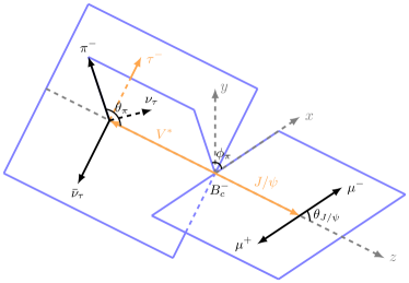
In order to distinguish between the SM and NP scenarios, and further characterise the underlying effects of NP, besides considering the total decay rate, the full angular distribution of and decays should also be taken into account sometimes, see for instance refs. Cohen:2018vhw ; Leljak:2019eyw ; Harrison:2020nrv . However, as pointed out in refs. Nierste:2008qe ; Tanaka:2010se ; Hagiwara:2014tsa ; Bordone:2016tex ; Alonso:2016gym ; Alonso:2017ktd ; Asadi:2018sym ; Alonso:2018vwa ; Bhattacharya:2020lfm ; Asadi:2020fdo ; Hu:2020axt ; Ligeti:2016npd , the information of the polar and azimuthal angles of the emitted cannot be determined precisely because the decay products of inevitably contain an undetected . This means that the observables depending on the polar or azimuthal angle of , such as the corresponding coefficients of the angular distribution and the forward-backward asymmetry of , cannot be directly measured. Therefore, in this work, we construct a measurable angular distribution by further considering the subsequent decay . The full cascade decay is , which includes three visible final-state particles , , and whose three-momenta can be measured. We first calculate the full five-fold differential angular distribution including all Lorentz structures of the NP effective operators, and then carefully study the NP effects in the angular distribution from many aspects.
Our paper is organized as follows. In section 2, after defining the effective Hamiltonian, we give the analytical results of the independent transversity amplitudes and the measurable angular distribution of the five-body decay. Definitions of the integrated observables are included in section 3. In section 4, we show the numerical results of the entire set of normalized angular observables and the lepton-flavor-universality ratios and . A model-independent method for determining the existence of tensor operator is given in section 5. Our conclusions are finally made in section 6. In the appendices A and B, we present the detailed procedures related to the calculations of angular distribution and dependence relations, respectively.
2 Analytical results
In this section, after giving some necessary definitions, we directly list the analytical results of angular distribution. The more detailed calculations, including some useful conventions, can be found in appendix A.
2.1 Effective Hamiltonian
Assuming that the NP scale is higher than the electroweak scale, one can integrate out the possible NP particles as well as the SM heavy particles — the , , the top quark, and the Higgs boson, thus obtaining the effective Hamiltonian suitable for describing the transition222Neutrinos are assumed to be left-handed in this work. The effective Hamiltonian containing right-handed neutrinos can be found in refs. Dutta:2013qaa ; Ligeti:2016npd ; Mandal:2020htr . It can be derived from the identity that the operator is absent. We use the convention .
| (1) |
where is the Fermi constant, is the CKM matrix element, , and denotes the field of left-handed neutrino. The NP effects are encoded in the Wilson coefficients , which are defined at the typical energy scale . In the SM, and .
2.2 Transversity amplitudes
In the calculation, the hadronic matrix elements contain the nonperturbative QCD effects and can be parameterized as the Lorentz invariant form factors. The vector and axial-vector current matrix elements can be written as the following four form factors Beneke:2000wa ; Sakaki:2013bfa ; Harrison:2020gvo
| (2) | ||||
| (3) |
where , denotes the polarization vector of meson. In our numerical analysis, we will use the vector and axial-vector form factors computed in lattice QCD Harrison:2020gvo ; Harrison:2020nrv .
Using the equation of motion, the scalar and pseudo-scalar matrix elements can be obtained by
| (4) | ||||
| (5) |
Based on the above four form factors and , one can define four independent transversity amplitudes as follows
| (6) | ||||
| (7) | ||||
| (8) | ||||
| (9) |
with
| (10) |
where and are the current quark masses evaluated at the scale , and .
The tensor matrix element can be parameterized as Beneke:2000wa ; Sakaki:2013bfa ; Leljak:2019eyw
| (11) |
and . In the presence of the tensor operators, we find three additional independent transversity amplitudes as follows
| (12) | ||||
| (13) | ||||
| (14) |
where the superscript indicates that an amplitude appears only when one considers the tensor operators.
2.3 Angular distribution
The measurable angular distribution of the five-body decay can be written as
| (15) |
where denotes the magnitude of three-momentum of the meson in the rest frame. and are the branching fractions of and decays, respectively. Here is the invariant mass squared of the pair; denotes the polar angle of in the rest frame; , , and represent the energy, polar angle, and azimuthal angle of in the center-of-mass frame, respectively. A more intuitive definition of the angles is shown in figure 1. The function can be decomposed into a set of trigonometric functions as follows
| (16) |
The twelve angular observables can be completely expressed in terms of the seven transversity amplitudes defined in subsection 2.2 and the dimensionless factors listed in appendix A.3. Explicitly, we have
| (17) | ||||
| (18) | ||||
| (19) | ||||
| (20) | ||||
| (21) | ||||
| (22) | ||||
| (23) | ||||
| (24) | ||||
| (25) | ||||
| (26) | ||||
| (27) | ||||
| (28) |
In the SM, the angular observables , , and are vanishing. Therefore, in future measurements, a non-vanishing , , or would be a solid signal of NP, which induces a complex contribution to the amplitude.
3 Integrated observables
3.1 -integrated angular observables
The differential decay rate (2.3) depends on five parameters , , , and , and a complete experimental analysis may be limited by statistics. Integrating over the and after a proper normalization, we can get the following angular function
| (29) |
with the twelve normalized angular observables defined as
| (30) |
Our choice of the normalization in eq. (3.1) results the relationship . The cancellations through normalization to the decay rate lead to the observation that the observables have less theoretical uncertainty to facilitate the discussion of the NP effects. In section 4, we will analyze numerically the entire set of observables within the SM and in some NP benchmark points.
The forward-backward asymmetry of meson as a function of can be defined as
| (31) |
This asymmetry observable only exists in channel, and specifically for the decay. Obviously, it can be expressed linearly in terms of angular observables .
By integrating over the lepton-side parameters , , , one can obtain the two-fold differential decay rate as follows
| (32) |
where
| (33) |
are the longitudinal and transverse polarization fractions of the meson, respectively. The differential decay rates for the longitudinally and transversely polarized intermediate state are given, respectively, by
| (34) | ||||
| (35) |
with the factor
| (36) |
The polarization observables constructed above are not affected by decay dynamics since we have integrated over all the lepton-side kinematic parameters, so they are also applicable to light leptons and . We denote and as extraction from and decays respectively, and define the following ratios to probe the universality of lepton flavor
| (37) |
The distribution of the decay rate can be obtained by adding up eqs. (34) and (35) as follows
| (38) |
Our (apart from ) is consistent with that in refs. Harrison:2020nrv ; Sakaki:2013bfa .
3.2 Tau asymmetries in from the visible kinematics
After integrating over the variables and , one has
| (39) |
This three-fold differential decay rate can be used to indirectly reveal the information of asymmetries in decay Kiers:1997zt ; Nierste:2008qe ; Tanaka:2010se ; Sakaki:2012ft ; Ivanov:2017mrj ; Alonso:2017ktd ; Asadi:2020fdo . The following discussion of this subsection will follow closely refs. Alonso:2017ktd ; Asadi:2020fdo , which give a detailed analysis of the properties in decays using .
The eq. (3.2) can be rewritten as
| (40) |
with
| (41) | ||||
| (42) | ||||
| (43) |
Here, are the Legendre functions, the and the following and are defined in eq. (111). The asymmetries , , , , , , and are defined in the section 2 of ref. Asadi:2020fdo . We find that the functions are given, respectively, by
| (44) | ||||||||
where is the cosine of the - opening angle in the center-of-mass frame Hu:2020axt , and
| (45) | ||||
| (46) | ||||
| (47) |
Neglecting the mass, our results are in agreement with those in refs. Alonso:2017ktd ; Asadi:2020fdo . The sign difference in is due to the different choice of reference direction. It should be pointed out that in the absence of , the differential forward-backward asymmetry (i.e. ) cannot be expressed in terms of and as given by eq. (16) of ref. Alonso:2017ktd .
4 Numerical results
4.1 The form factors
The transition form factors are the main source of theoretical uncertainties. For the vector and axial-vector form factors, and , we use the latest high-precision lattice QCD calculation results given in ref. Harrison:2020gvo . Since the tensor form factors are not included in ref. Harrison:2020gvo , we will adopt the calculated in the QCD sum rule method Leljak:2019eyw .333We are very grateful to Domagoj Leljak for providing us with the variances and correlation matrix of -expansion parameters of tensor form factors. These form factors are parameterized in a simplified expansion to extend to the full range.
4.2 The NP benchmark points
The model-independent analyses of NP effects in decays have been completed in many previous works Alok:2017qsi ; Hu:2018veh ; Alok:2019uqc ; Murgui:2019czp ; Blanke:2018yud ; Blanke:2019qrx ; Shi:2019gxi ; Cheung:2020sbq ; Kumbhakar:2020jdz . In order to show the influences of these NP effects on the angular distribution of decay, we select various best-fit values as the NP benchmark points. These best-fit values are usually performed on a set of chiral base, which is equivalent to Eq. (2.1) by the following relations
| (48) | |||||||
According to the following steps, we select a total of eight NP benchmark points under seven different NP hypotheses.
Switching one coupling at a time, there are five NP hypotheses. The hypothesis of a single can resolve the anomalies well, but there is no effect on the normalized observables defined in section 3, so we should not choose it. The hypothesis of a single or is ruled out by the decay rate of decay Li:2016vvp ; Celis:2016azn ; Alonso:2016oyd . We take a benchmark point from each of the two remaining NP hypotheses as follows Cheung:2020sbq
The corresponding complex-conjugated fitting values and are marked as BP1∗ and BP2∗, respectively. Although BP1 (BP2) and BP1∗ (BP2∗) are formally different benchmark points, they produce the same results for angular observables and opposite results for . Observables can distinguish between the NP benchmark point and its complex conjugate partner very well. In the following analysis, we do not consider BP1∗ and BP2∗, and the same treatment is also applicable to the following BP6∗, which is the complex conjugate of the benchmark point BP6.
Considering the combinations induced by specific UV models, we choose the best-fit points in the following four different NP hypotheses as our NP benchmark points (the remaining are set to zero in each case) Blanke:2019qrx
| BP3: | |||
| BP4: | |||
| BP5: | |||
| BP6: |
where the Wilson coefficients are given at the NP scale 1TeV, and we should run them down to the scale Blanke:2018yud .
Finally, taking into account all NP Wilson coefficients, except which is explicitly lepton-flavor universal in the standard model effective field theory formalism up to contributions of Hu:2018veh , we choose a set of values labelled “Min 1b” in table 8 of ref. Murgui:2019czp as our NP benchmark point BP7
We adopt the same treatment as in many literatures (e.g. Becirevic:2019tpx ; Boer:2019zmp ; Asadi:2020fdo ; Harrison:2020nrv ; Alguero:2020ukk ), that is, only the central value of best-fit result is considered as the benchmark point to qualitatively discuss the influence of the NP effect.
4.3 Angular observables
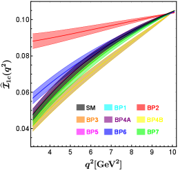
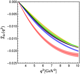

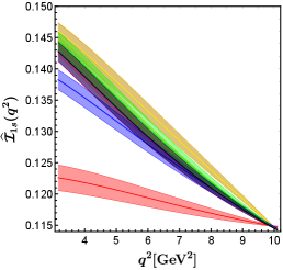
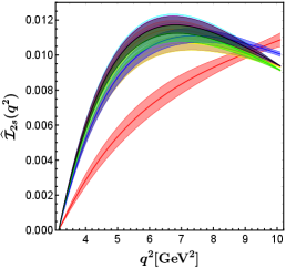

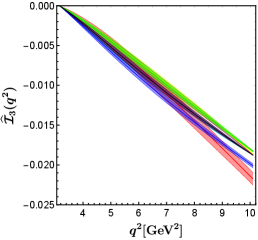
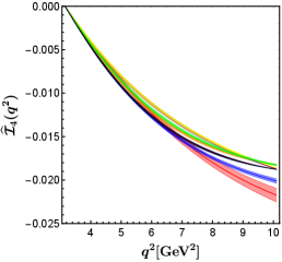

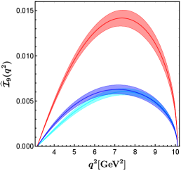
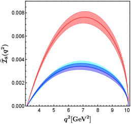
In figure 2, we show the predictions for the entire set of angular observables within the SM and in eight NP benchmark points. It is easy to see that the BP2 (corresponding to the red band in figure 2) has the greatest effect on all except . The value of in BP2 is almost the same as that in the SM. The NP corresponding to BP2 even makes the angular observables negative, which is not present in the SM and in other NP benchmark points.
In the BP6 (corresponding to the blue band in figure 2), the contributions of NP to all except are in the same direction as in BP2, but the impacts are smaller than that in BP2. The BP6 can obviously decrease the value of . Observables sensitive to BP6 can be used to study specific UV models, such as the scalar doublet (also called ) leptoquark Becirevic:2018afm , which can produce the relationship at the NP scale.
As we expected, only BP1, BP2, and BP6 which can provide complex phases can produce nonzero angular observables . The BP1 (corresponding to the cyan band in figure 2) makes decrease slightly, and hardly contributes to . The results of all predicted by BP4A and BP4B (corresponding to the purple and yellow bands in figure 2, respectively) coincide almost completely with each other. This indicates that cannot be used to distinguish the two best-fit points of NP hypothesis , which is motivated by models with extra charged Higgs. This is different from the situation in the angular observables of decay, which can distinguish between BP4A and BP4B very well Hu:2020axt . The BP4A and BP4B make decrease slightly and increase slightly. The NP effects of BP3, BP5, and BP7 have little impact on .
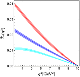
4.4 Lepton-flavor-universality ratios and
The distribution of lepton-flavor-universality ratios is shown in figure 3, which includes the results within the SM and in eight NP benchmark points. All NP benchmark points except BP5 and BP1 can be distinguished by , especially in the small region. The results of predicted by BP4A and BP4B coincide almost completely with each other. The longitudinal polarization ratio is decreased by benchmarks BP2 and BP6, and increased by benchmarks BP4A, BP4B, BP7, and BP3. Especially, the NP effect of BP2 makes the ratio significantly less than 1. The transverse polarization ratio is increased by benchmarks BP2 and BP6, and decreased by benchmarks BP4A, BP4B, BP7, and BP3. The NP effect of BP2 makes the ratio significantly greater than 1.
All of the NP benchmark points can increase the ratio . does not use the channel for normalization, so the contribution of BP3, BP5, and BP7 can be seen. The predicted values of are shown as follows
| (49) | ||||||||
5 Symmetries in the angular observables without tensor operators
In the absence of tensor operators, the twelve angular observables defined in section 2.3 are not independent. These angular observables change to
| (50) | ||||
| (51) | ||||
| (52) | ||||
| (53) | ||||
| (54) | ||||
| (55) | ||||
| (56) | ||||
| (57) | ||||
| (58) | ||||
| (59) | ||||
| (60) | ||||
| (61) |
We can consider these angular observables as being bilinear in
| (62) |
Generally, the experimental and theoretical degrees of freedom can be matched by the following formula Egede:2010zc ; Matias:2012xw ; Hofer:2015kka ; Alguero:2020ukk
| (63) |
where is the number of angular observables ; is the number of dependencies between the different observables , which can be obtained by the difference between the number of observables and the dimension of the space given by the gradient vectors (with the derivatives taken with respect to the various elements of ); is the number of transversity amplitudes (each is complex and therefore has two degrees of freedom); is the number of continuous symmetries.
Without tensor operators, there are still twelve angular observables but only four amplitudes . So and . In this case, the only continuous symmetry that can be found is
| (64) |
Only 7 of the 12 angular observables are independent and 5 dependencies are found. We present the dependence relations directly here and provide the detailed derivation in appendix B:
| (65) | ||||
| (66) | ||||
| (67) | ||||
| (68) | ||||
| (69) |
with
| (70) | ||||
| (71) |
Eqs. (65)–(69) can be used as a model-independent method to determine the existence of tensor operators. The “model-independent method” here not only means that it does not depend on the NP models, but also means that it does not depend on the calculation of transition form factors.
6 Conclusions
Inspired by the anomalies, the angular distribution of or decay has been used to explore possible NP patterns in transition in many previous works. However, angular observables depending on the solid angle of final-state are unmeasurable theoretically, since the decay products of inevitably contain an undetected and the solid angle of cannot be determined precisely. Therefore, in this work, we study the measurable angular distribution of the five-body decay , which includes three visible final-state particles , , and , with their three-momenta all being measured.
The five-fold differential decay rate containing all NP effective operators can be expressed in terms of twelve angular observables , which can be completely expressed by seven independent transversity amplitudes and some dimensionless factors. As long as one of the angular observables , and is nonzero, this will be an unquestionable sign of NP, and indicates that the NP can cause extra weak phases. Integrating the five-fold differential decay rate over the and normalized by , we can construct twelve normalized angular observables . By integrating over all lepton-side parameters, we find that there are only two angular observables whose determination can be obtained without reconstruction of the dilepton solid angle. The are not affected by the lepton dynamics, so they can be used to construct the ratios to probe the universality of lepton flavor. Based on our five-fold differential decay rate, we show how to extract the complete set of asymmetries in decay from the visible final-state kinematics.
Using the vector and axial-vector form factors calculated by the latest lattice QCD and the tensor form factors calculated by the QCD sum rule, we predict the distribution of the twelve normalized angular observables and the two lepton-flavor-universality ratios both within the SM and in eight NP benchmark points, which are a variety of best-fit points in seven different NP hypotheses. We find that the benchmark BP2 (corresponding to the hypothesis of tensor operator) has the greatest effect on all and , except . Especially for the observables and , BP2 makes their predictions very different from those in the SM and other benchmark points. The results of all and predicted by the two best-fit points (i.e. BP4A and BP4B) of NP hypothesis , which is motivated by models with extra charged Higgs, coincide almost completely with each other. This is different from the situation in the angular observables of the baryonic counterparts, which can distinguish between BP4A and BP4B very well. In addition to the benchmarks BP2, BP4A, and BP4B, the BP1, BP6, and BP7 can also have some influence on the observables. Compared with the , the ratios are more sensitive to the NP with pseudo-scalar operator. All NP benchmark points can improve the value of , which makes it closer to the experimental measurement.
We discuss the symmetries in the angular observables without tensor operators, and present five dependence relations. Once all twelve angular observables are measured, these five relations will be a very useful way to determine the existence of tensor operators. If these relations are not fulfilled, it means that there must be tensor operators. This method is completely independent of any assumptions on the details of the NP model and transition form factors.
The cascade decay provides a good prospect for measurement by the LHCb experiment, because it has excellent final-state signatures with a strongly peaking spectrum and a well identification. Additionally, the lifetime of meson is almost three times shorter than that of mesons, which can be used to improve the separation of decay from decays, thus providing an extra handle to distinguish the large background that derives from the mesons Aaij:2017tyk ; Bernlochner:2021vlv . One possible background is the very rare decay Aaij:2015nea , which has about one-tenth the number of events as the signal decay. This background can also be distinguished from the signal by the kinematic properties of the visible final-state particles. Future precise measurements of the angular observables in decay, especially precise measurements of the normalized ones, would be very helpful to provide a more definite answer concerning the anomalies observed in transition, restricting further or even deciphering the NP models.
Acknowledgements.
This work is supported by the National Natural Science Foundation of China under Grant Nos. 11947083, 12075097, 11675061 and 11775092, as well as by the CCNU-QLPL Innovation Fund (QLPL2020P01). X.L. is also supported by the Fundamental Research Funds for the Central Universities under Grant No. CCNU20TS007.Appendix A The calculation of the angular distribution
In the appendix of ref. Hu:2020axt , we have given the detailed calculation procedures for the similar five-body cascade decay of unpolarized baryon. The calculation of part is exactly the same as that in this work. Therefore, in this section, we mainly present some important definitions and conventions, and calculate the decay. At the end of this section, the dimensionless factors are listed for the sake of completeness of this paper.
A.1 Definitions and conventions
The differential decay rate of cascade decay can be written as
| (73) |
where
| (74) | ||||
| (75) | ||||
| (76) | ||||
| (77) |
The and respectively represent the helicity of final-state particles and , as well as the and respectively represent the helicity of intermediate state and . The stands for the two-body phase space. denotes the helicity amplitude related to decay. are the hadronic helicity amplitudes describing the transition with different Lorentz structures.
| (78) | ||||
| (79) | ||||
| (80) |
where denotes the polarization vector of the virtual vector boson with helicity . The modified leptonic helicity amplitudes are , which can be obtained directly from the appendix of ref. Hu:2020axt .
In the rest frame, the polarization vector of meson can be written as Auvil:1966eao ; Haber:1994pe
| (81) | ||||
| (82) |
with and . The polarization vector of virtual can be written as Auvil:1966eao ; Haber:1994pe
| (83) | ||||
| (84) | ||||
| (85) |
with and . Eqs. (83)–(85) satisfy the completeness relation
| (86) |
where and .
For scalar and pseudo-scalar operators, there is only one nonzero hadronic helicity amplitude
| (87) |
For vector and axial-vector operators, there are four nonzero hadronic helicity amplitudes listed as follows
| (88) |
For the tensor operators, there are twelve nonzero hadronic helicity amplitudes listed as follows
| (89) |
A.2 Calculating decay
The decay should be calculated in the rest frame. In this reference frame, the transverse polarization vector of meson does not change, i.e., , but its longitudinal polarization vector changes to . For massless and leptons, their spinors can be written as Auvil:1966eao ; Haber:1994pe
| (90) | ||||
| (91) | ||||
| (92) | ||||
| (93) |
where the Jacob-Wick second particle convention has been used Jacob:1959at .
As the decay is dominated by electromagnetic interaction, we can write the helicity amplitude as follows
| (94) |
where , is the decay constant of meson, is the fine-structure constant. There are six nonzero helicity amplitudes as follows
| (95) | ||||
| (96) | ||||
| (97) |
and one can obtain that the total decay rate is
| (98) |
A.3 Dimensionless factors
The dimensionless factors induced in the calculation of are as follows Hu:2020axt
| (99) | ||||
| (100) | ||||
| (101) | ||||
| (102) | ||||
| (103) | ||||
| (104) | ||||
| (105) | ||||
| (106) | ||||
| (107) | ||||
| (108) | ||||
| (109) | ||||
| (110) |
where the three dimensionless parameters are defined as
| (111) |
In the limit , the -integrated factors are given, respectively, by
| (112) | ||||
| (113) | ||||
| (114) | ||||
| (115) | ||||
| (116) | ||||
| (117) | ||||
| (118) | ||||
| (119) | ||||
| (120) | ||||
| (121) | ||||
| (122) | ||||
| (123) |
We provide the full analytical results for these factors electronically in the supplementary material.
Appendix B The detailed derivation of the dependence relations
In this section we provide the detailed derivation of the dependence relations among the angular observables . It is useful to re-express , , and as
| (124) | ||||
| (125) | ||||
| (126) | ||||
| (127) |
Therefore, the twelve angular observables (50)–(61) can be seen as functions of 4 real variables , , , and 3 complex variables , , . The advantage of this view is that it implies the continuous symmetry (64). There are only seven independent real variables due to the following three relationships
| (128) | ||||
| (129) | ||||
| (130) |
Inverting the eqs. (51)–(60), one can rewrite the variables in terms of the angular observables as follows
| (131) | ||||
| (132) | ||||
| (133) | ||||
| (134) | ||||
| (135) | ||||
| (136) | ||||
| (137) | ||||
| (138) | ||||
| (139) | ||||
| (140) |
with and defined in eqs. (70) and (71), respectively. Substituting them into eqs. (50), (61), and (128)–(130), we can obtain the final form of the 5 dependence relations (65)–(69).
References
- (1) ATLAS collaboration, Observation of a new particle in the search for the Standard Model Higgs boson with the ATLAS detector at the LHC, Phys. Lett. B 716 (2012) 1 [1207.7214].
- (2) CMS collaboration, Observation of a New Boson at a Mass of 125 GeV with the CMS Experiment at the LHC, Phys. Lett. B 716 (2012) 30 [1207.7235].
- (3) ATLAS, CMS collaboration, Combined Measurement of the Higgs Boson Mass in Collisions at and 8 TeV with the ATLAS and CMS Experiments, Phys. Rev. Lett. 114 (2015) 191803 [1503.07589].
- (4) BaBar collaboration, Evidence for an excess of decays, Phys. Rev. Lett. 109 (2012) 101802 [1205.5442].
- (5) BaBar collaboration, Measurement of an Excess of Decays and Implications for Charged Higgs Bosons, Phys. Rev. D 88 (2013) 072012 [1303.0571].
- (6) LHCb collaboration, Measurement of the ratio of branching fractions , Phys. Rev. Lett. 115 (2015) 111803 [1506.08614].
- (7) Belle collaboration, Measurement of the branching ratio of relative to decays with hadronic tagging at Belle, Phys. Rev. D 92 (2015) 072014 [1507.03233].
- (8) Belle collaboration, Measurement of the lepton polarization and in the decay , Phys. Rev. Lett. 118 (2017) 211801 [1612.00529].
- (9) LHCb collaboration, Measurement of the ratio of the and branching fractions using three-prong -lepton decays, Phys. Rev. Lett. 120 (2018) 171802 [1708.08856].
- (10) Belle collaboration, Measurement of the lepton polarization and in the decay with one-prong hadronic decays at Belle, Phys. Rev. D 97 (2018) 012004 [1709.00129].
- (11) LHCb collaboration, Test of Lepton Flavor Universality by the measurement of the branching fraction using three-prong decays, Phys. Rev. D 97 (2018) 072013 [1711.02505].
- (12) Belle collaboration, Measurement of and with a semileptonic tagging method, Phys. Rev. Lett. 124 (2020) 161803 [1910.05864].
- (13) HFLAV collaboration, Averages of -hadron, -hadron, and -lepton properties as of 2018, 1909.12524.
- (14) HFLAV collaboration, Online update for averages of and for Spring 2019 at https://hflav-eos.web.cern.ch/hflav-eos/semi/spring19/html/RDsDsstar/RDRDs.html, .
- (15) M. Bordone, M. Jung and D. van Dyk, Theory determination of form factors at , Eur. Phys. J. C 80 (2020) 74 [1908.09398].
- (16) F.U. Bernlochner, M.F. Sevilla, D.J. Robinson and G. Wormser, Semitauonic -hadron decays: A lepton flavor universality laboratory, 2101.08326.
- (17) A.K. Alok, D. Kumar, J. Kumar, S. Kumbhakar and S.U. Sankar, New physics solutions for and , JHEP 09 (2018) 152 [1710.04127].
- (18) Q.-Y. Hu, X.-Q. Li and Y.-D. Yang, transitions in the standard model effective field theory, Eur. Phys. J. C 79 (2019) 264 [1810.04939].
- (19) A.K. Alok, D. Kumar, S. Kumbhakar and S. Uma Sankar, Solutions to - in light of Belle 2019 data, Nucl. Phys. B 953 (2020) 114957 [1903.10486].
- (20) C. Murgui, A. Peñuelas, M. Jung and A. Pich, Global fit to transitions, JHEP 09 (2019) 103 [1904.09311].
- (21) M. Blanke, A. Crivellin, S. de Boer, T. Kitahara, M. Moscati, U. Nierste et al., Impact of polarization observables and on new physics explanations of the anomaly, Phys. Rev. D 99 (2019) 075006 [1811.09603].
- (22) M. Blanke, A. Crivellin, T. Kitahara, M. Moscati, U. Nierste and I. Nišandžić, Addendum to “Impact of polarization observables and on new physics explanations of the anomaly”, 1905.08253.
- (23) R.-X. Shi, L.-S. Geng, B. Grinstein, S. Jäger and J. Martin Camalich, Revisiting the new-physics interpretation of the data, JHEP 12 (2019) 065 [1905.08498].
- (24) K. Cheung, Z.-R. Huang, H.-D. Li, C.-D. Lü, Y.-N. Mao and R.-Y. Tang, Revisit to the transition: In and beyond the SM, Nucl. Phys. B 965 (2021) 115354 [2002.07272].
- (25) S. Kumbhakar, Signatures of complex new physics in transitions, Nucl. Phys. B 963 (2021) 115297 [2007.08132].
- (26) M. Tanaka and R. Watanabe, New physics in the weak interaction of , Phys. Rev. D 87 (2013) 034028 [1212.1878].
- (27) Y. Sakaki, M. Tanaka, A. Tayduganov and R. Watanabe, Testing leptoquark models in , Phys. Rev. D 88 (2013) 094012 [1309.0301].
- (28) M. Bauer and M. Neubert, Minimal Leptoquark Explanation for the R , RK , and Anomalies, Phys. Rev. Lett. 116 (2016) 141802 [1511.01900].
- (29) S. Fajfer and N. Košnik, Vector leptoquark resolution of and puzzles, Phys. Lett. B 755 (2016) 270 [1511.06024].
- (30) X.-Q. Li, Y.-D. Yang and X. Zhang, Revisiting the one leptoquark solution to the anomalies and its phenomenological implications, JHEP 08 (2016) 054 [1605.09308].
- (31) A. Crivellin, D. Müller and T. Ota, Simultaneous explanation of and : the last scalar leptoquarks standing, JHEP 09 (2017) 040 [1703.09226].
- (32) D. Bečirević, I. Doršner, S. Fajfer, N. Košnik, D.A. Faroughy and O. Sumensari, Scalar leptoquarks from grand unified theories to accommodate the -physics anomalies, Phys. Rev. D 98 (2018) 055003 [1806.05689].
- (33) A. Angelescu, D. Bečirević, D. Faroughy and O. Sumensari, Closing the window on single leptoquark solutions to the -physics anomalies, JHEP 10 (2018) 183 [1808.08179].
- (34) S. Bansal, R.M. Capdevilla and C. Kolda, Constraining the minimal flavor violating leptoquark explanation of the anomaly, Phys. Rev. D 99 (2019) 035047 [1810.11588].
- (35) S. Iguro, T. Kitahara, Y. Omura, R. Watanabe and K. Yamamoto, D∗ polarization vs. anomalies in the leptoquark models, JHEP 02 (2019) 194 [1811.08899].
- (36) A. Crivellin, D. Müller and F. Saturnino, Flavor Phenomenology of the Leptoquark Singlet-Triplet Model, JHEP 06 (2020) 020 [1912.04224].
- (37) N. Deshpande and X.-G. He, Consequences of R-parity violating interactions for anomalies in and , Eur. Phys. J. C 77 (2017) 134 [1608.04817].
- (38) W. Altmannshofer, P. Bhupal Dev and A. Soni, anomaly: A possible hint for natural supersymmetry with -parity violation, Phys. Rev. D 96 (2017) 095010 [1704.06659].
- (39) Q.-Y. Hu, X.-Q. Li, Y. Muramatsu and Y.-D. Yang, R-parity violating solutions to the anomaly and their GUT-scale unifications, Phys. Rev. D 99 (2019) 015008 [1808.01419].
- (40) Q.-Y. Hu, Y.-D. Yang and M.-D. Zheng, Revisiting the -physics anomalies in -parity violating MSSM, Eur. Phys. J. C 80 (2020) 365 [2002.09875].
- (41) W. Altmannshofer, P.B. Dev, A. Soni and Y. Sui, Addressing R, R, muon and ANITA anomalies in a minimal -parity violating supersymmetric framework, Phys. Rev. D 102 (2020) 015031 [2002.12910].
- (42) A. Crivellin, C. Greub and A. Kokulu, Explaining , and in a 2HDM of type III, Phys. Rev. D 86 (2012) 054014 [1206.2634].
- (43) A. Celis, M. Jung, X.-Q. Li and A. Pich, Sensitivity to charged scalars in and decays, JHEP 01 (2013) 054 [1210.8443].
- (44) P. Ko, Y. Omura and C. Yu, and in chiral models with flavored multi Higgs doublets, JHEP 03 (2013) 151 [1212.4607].
- (45) A. Celis, M. Jung, X.-Q. Li and A. Pich, Scalar contributions to transitions, Phys. Lett. B 771 (2017) 168 [1612.07757].
- (46) S. Iguro and K. Tobe, in a general two Higgs doublet model, Nucl. Phys. B 925 (2017) 560 [1708.06176].
- (47) S. Iguro and Y. Omura, Status of the semileptonic decays and muon g-2 in general 2HDMs with right-handed neutrinos, JHEP 05 (2018) 173 [1802.01732].
- (48) P. Asadi, M.R. Buckley and D. Shih, It’s all right(-handed neutrinos): a new model for the anomaly, JHEP 09 (2018) 010 [1804.04135].
- (49) A. Greljo, D.J. Robinson, B. Shakya and J. Zupan, from and right-handed neutrinos, JHEP 09 (2018) 169 [1804.04642].
- (50) K. Babu, B. Dutta and R.N. Mohapatra, A theory of anomaly with right-handed currents, JHEP 01 (2019) 168 [1811.04496].
- (51) M. Blanke and A. Crivellin, Meson Anomalies in a Pati-Salam Model within the Randall-Sundrum Background, Phys. Rev. Lett. 121 (2018) 011801 [1801.07256].
- (52) S. Iguro, J. Kawamura, S. Okawa and Y. Omura, TeV-scale vector leptoquark from Pati-Salam unification with vectorlike families, 2103.11889.
- (53) LHCb collaboration, Measurement of the ratio of branching fractions , Phys. Rev. Lett. 120 (2018) 121801 [1711.05623].
- (54) LATTICE-HPQCD collaboration, and Lepton Flavor Universality Violating Observables from Lattice QCD, Phys. Rev. Lett. 125 (2020) 222003 [2007.06956].
- (55) HPQCD collaboration, form factors for the full range from lattice QCD, Phys. Rev. D 102 (2020) 094518 [2007.06957].
- (56) R. Watanabe, New Physics effect on in relation to the anomaly, Phys. Lett. B 776 (2018) 5 [1709.08644].
- (57) J. Zhu, B. Wei, J.-H. Sheng, R.-M. Wang, Y. Gao and G.-R. Lu, Probing the R-parity violating supersymmetric effects in and decays, Nucl. Phys. B 934 (2018) 380 [1801.00917].
- (58) C.-T. Tran, M.A. Ivanov, J.G. Körner and P. Santorelli, Implications of new physics in the decays , Phys. Rev. D 97 (2018) 054014 [1801.06927].
- (59) A. Issadykov and M.A. Ivanov, The decays and in covariant confined quark model, Phys. Lett. B 783 (2018) 178 [1804.00472].
- (60) T.D. Cohen, H. Lamm and R.F. Lebed, Tests of the standard model in , and , Phys. Rev. D 98 (2018) 034022 [1807.00256].
- (61) T.D. Cohen, H. Lamm and R.F. Lebed, Model-independent bounds on , JHEP 09 (2018) 168 [1807.02730].
- (62) Z.-R. Huang, Y. Li, C.-D. Lu, M.A. Paracha and C. Wang, Footprints of New Physics in Transitions, Phys. Rev. D 98 (2018) 095018 [1808.03565].
- (63) W. Wang and R. Zhu, Model independent investigation of the and ratios of decay widths of semileptonic decays into a P-wave charmonium, Int. J. Mod. Phys. A 34 (2019) 1950195 [1808.10830].
- (64) D. Leljak, B. Melic and M. Patra, On lepton flavour universality in semileptonic decays, JHEP 05 (2019) 094 [1901.08368].
- (65) X.-Q. Hu, S.-P. Jin and Z.-J. Xiao, Semileptonic decays in the ”PQCD + Lattice” approach, Chin. Phys. C 44 (2020) 023104 [1904.07530].
- (66) K. Azizi, Y. Sarac and H. Sundu, Lepton flavor universality violation in semileptonic tree level weak transitions, Phys. Rev. D 99 (2019) 113004 [1904.08267].
- (67) N. Penalva, E. Hernández and J. Nieves, , and semileptonic decays including new physics, Phys. Rev. D 102 (2020) 096016 [2007.12590].
- (68) A. Berns and H. Lamm, Model-Independent Prediction of , JHEP 12 (2018) 114 [1808.07360].
- (69) C.W. Murphy and A. Soni, Model-Independent Determination of Form Factors, Phys. Rev. D 98 (2018) 094026 [1808.05932].
- (70) R. Dutta, decays within standard model and beyond, Phys. Rev. D 93 (2016) 054003 [1512.04034].
- (71) X.-Q. Li, Y.-D. Yang and X. Zhang, decay in scalar and vector leptoquark scenarios, JHEP 02 (2017) 068 [1611.01635].
- (72) E. Di Salvo, F. Fontanelli and Z. Ajaltouni, Detailed Study of the Decay , Int. J. Mod. Phys. A 33 (2018) 1850169 [1804.05592].
- (73) A. Ray, S. Sahoo and R. Mohanta, Probing new physics in semileptonic decays, Phys. Rev. D 99 (2019) 015015 [1812.08314].
- (74) N. Penalva, E. Hernández and J. Nieves, Further tests of lepton flavour universality from the charged lepton energy distribution in semileptonic decays: The case of , Phys. Rev. D 100 (2019) 113007 [1908.02328].
- (75) X.-L. Mu, Y. Li, Z.-T. Zou and B. Zhu, Investigation of effects of new physics in decay, Phys. Rev. D 100 (2019) 113004 [1909.10769].
- (76) T. Gutsche, M.A. Ivanov, J.G. Körner, V.E. Lyubovitskij, P. Santorelli and N. Habyl, Semileptonic decay in the covariant confined quark model, Phys. Rev. D 91 (2015) 074001 [1502.04864].
- (77) S. Shivashankara, W. Wu and A. Datta, Decay in the Standard Model and with New Physics, Phys. Rev. D 91 (2015) 115003 [1502.07230].
- (78) P. Böer, A. Kokulu, J.-N. Toelstede and D. van Dyk, Angular Analysis of , JHEP 12 (2019) 082 [1907.12554].
- (79) M. Ferrillo, A. Mathad, P. Owen and N. Serra, Probing effects of new physics in decays, JHEP 12 (2019) 148 [1909.04608].
- (80) Q.-Y. Hu, X.-Q. Li, Y.-D. Yang and D.-H. Zheng, The measurable angular distribution of decay, JHEP 02 (2021) 183 [2011.05912].
- (81) R. Dutta, Phenomenology of decays, Phys. Rev. D 97 (2018) 073004 [1801.02007].
- (82) R. Faustov and V. Galkin, Relativistic description of the baryon semileptonic decays, Phys. Rev. D 98 (2018) 093006 [1810.03388].
- (83) J. Zhang, J. Su and Q. Zeng, Contributions of vector leptoquark to decay, Nucl. Phys. B 938 (2019) 131.
- (84) J. Zhang, X. An, R. Sun and J. Su, Probing new physics in semileptonic decays, Eur. Phys. J. C 79 (2019) 863.
- (85) N. Rajeev, R. Dutta and S. Kumbhakar, Implication of anomalies on semileptonic decays of and baryons, Phys. Rev. D 100 (2019) 035015 [1905.13468].
- (86) J.-H. Sheng, J. Zhu, X.-N. Li, Q.-Y. Hu and R.-M. Wang, Probing new physics in semileptonic and decays, Phys. Rev. D 102 (2020) 055023 [2009.09594].
- (87) V.V. Kiselev, A.K. Likhoded and A.I. Onishchenko, Semileptonic meson decays in sum rules of QCD and NRQCD, Nucl. Phys. B569 (2000) 473 [hep-ph/9905359].
- (88) M.A. Ivanov, J.G. Korner and P. Santorelli, The Semileptonic decays of the meson, Phys. Rev. D63 (2001) 074010 [hep-ph/0007169].
- (89) D. Ebert, R.N. Faustov and V.O. Galkin, Weak decays of the meson to charmonium and mesons in the relativistic quark model, Phys. Rev. D68 (2003) 094020 [hep-ph/0306306].
- (90) E. Hernandez, J. Nieves and J.M. Verde-Velasco, Study of exclusive semileptonic and non-leptonic decays of - in a nonrelativistic quark model, Phys. Rev. D74 (2006) 074008 [hep-ph/0607150].
- (91) M.A. Ivanov, J.G. Körner and P. Santorelli, Exclusive semileptonic and nonleptonic decays of the meson, Phys. Rev. D73 (2006) 054024 [hep-ph/0602050].
- (92) W. Wang, Y.-L. Shen and C.-D. Lu, Covariant Light-Front Approach for transition form factors, Phys. Rev. D79 (2009) 054012 [0811.3748].
- (93) C.-F. Qiao and R.-L. Zhu, Estimation of semileptonic decays of meson to S-wave charmonia with nonrelativistic QCD, Phys. Rev. D87 (2013) 014009 [1208.5916].
- (94) W.-F. Wang, Y.-Y. Fan and Z.-J. Xiao, Semileptonic decays in the perturbative QCD approach, Chin. Phys. C37 (2013) 093102 [1212.5903].
- (95) Z. Rui, H. Li, G.-x. Wang and Y. Xiao, Semileptonic decays of meson to S-wave charmonium states in the perturbative QCD approach, Eur. Phys. J. C76 (2016) 564 [1602.08918].
- (96) R. Dutta and A. Bhol, semileptonic decays within the standard model and beyond, Phys. Rev. D96 (2017) 076001 [1701.08598].
- (97) HPQCD collaboration, decays from highly improved staggered quarks and NRQCD, PoS LATTICE2016 (2016) 281 [1611.01987].
- (98) A. Lytle, B. Colquhoun, C. Davies, J. Koponen and C. McNeile, Semileptonic decays from full lattice QCD, PoS BEAUTY2016 (2016) 069 [1605.05645].
- (99) U. Nierste, S. Trine and S. Westhoff, Charged-Higgs effects in a new differential decay distribution, Phys. Rev. D 78 (2008) 015006 [0801.4938].
- (100) M. Tanaka and R. Watanabe, Tau longitudinal polarization in and its role in the search for charged Higgs boson, Phys. Rev. D 82 (2010) 034027 [1005.4306].
- (101) K. Hagiwara, M.M. Nojiri and Y. Sakaki, violation in using multipion tau decays, Phys. Rev. D 89 (2014) 094009 [1403.5892].
- (102) M. Bordone, G. Isidori and D. van Dyk, Impact of leptonic decays on the distribution of decays, Eur. Phys. J. C 76 (2016) 360 [1602.06143].
- (103) R. Alonso, A. Kobach and J. Martin Camalich, New physics in the kinematic distributions of , Phys. Rev. D 94 (2016) 094021 [1602.07671].
- (104) R. Alonso, J. Martin Camalich and S. Westhoff, Tau properties in from visible final-state kinematics, Phys. Rev. D 95 (2017) 093006 [1702.02773].
- (105) P. Asadi, M.R. Buckley and D. Shih, Asymmetry Observables and the Origin of Anomalies, Phys. Rev. D 99 (2019) 035015 [1810.06597].
- (106) R. Alonso, J. Martin Camalich and S. Westhoff, Tau Polarimetry in B Meson Decays, SciPost Phys. Proc. 1 (2019) 012 [1811.05664].
- (107) B. Bhattacharya, A. Datta, S. Kamali and D. London, A measurable angular distribution for decays, JHEP 07 (2020) 194 [2005.03032].
- (108) P. Asadi, A. Hallin, J. Martin Camalich, D. Shih and S. Westhoff, Complete framework for tau polarimetry in decays, Phys. Rev. D 102 (2020) 095028 [2006.16416].
- (109) Z. Ligeti, M. Papucci and D.J. Robinson, New Physics in the Visible Final States of , JHEP 01 (2017) 083 [1610.02045].
- (110) R. Dutta, A. Bhol and A.K. Giri, Effective theory approach to new physics in and leptonic and semileptonic decays, Phys. Rev. D 88 (2013) 114023 [1307.6653].
- (111) R. Mandal, C. Murgui, A. Peñuelas and A. Pich, The role of right-handed neutrinos in anomalies, JHEP 08 (2020) 022 [2004.06726].
- (112) M. Beneke and T. Feldmann, Symmetry breaking corrections to heavy to light B meson form-factors at large recoil, Nucl. Phys. B 592 (2001) 3 [hep-ph/0008255].
- (113) K. Kiers and A. Soni, Improving constraints on tan Beta / m() using anti-neutrino, Phys. Rev. D 56 (1997) 5786 [hep-ph/9706337].
- (114) Y. Sakaki and H. Tanaka, Constraints on the charged scalar effects using the forward-backward asymmetry on , Phys. Rev. D 87 (2013) 054002 [1205.4908].
- (115) M.A. Ivanov, J.G. Körner and C.-T. Tran, Probing new physics in using the longitudinal, transverse, and normal polarization components of the tau lepton, Phys. Rev. D 95 (2017) 036021 [1701.02937].
- (116) R. Alonso, B. Grinstein and J. Martin Camalich, Lifetime of Constrains Explanations for Anomalies in , Phys. Rev. Lett. 118 (2017) 081802 [1611.06676].
- (117) D. Bečirević, M. Fedele, I. Nišandžić and A. Tayduganov, Lepton Flavor Universality tests through angular observables of decay modes, 1907.02257.
- (118) M. Algueró, S. Descotes-Genon, J. Matias and M. Novoa-Brunet, Symmetries in angular observables, JHEP 06 (2020) 156 [2003.02533].
- (119) U. Egede, T. Hurth, J. Matias, M. Ramon and W. Reece, New physics reach of the decay mode , JHEP 10 (2010) 056 [1005.0571].
- (120) J. Matias, F. Mescia, M. Ramon and J. Virto, Complete Anatomy of and its angular distribution, JHEP 04 (2012) 104 [1202.4266].
- (121) L. Hofer and J. Matias, Exploiting the symmetries of P and S wave for , JHEP 09 (2015) 104 [1502.00920].
- (122) LHCb collaboration, First measurement of the differential branching fraction and asymmetry of the decay, JHEP 10 (2015) 034 [1509.00414].
- (123) P. Auvil and J. Brehm, Wave Functions for Particles of Higher Spin, Phys. Rev. 145 (1966) 1152.
- (124) H.E. Haber, Spin formalism and applications to new physics searches, in 21st Annual SLAC Summer Institute on Particle Physics: Spin Structure in High-energy Processes (School: 26 Jul - 3 Aug, Topical Conference: 4-6 Aug) (SSI 93), pp. 231–272, 4, 1994 [hep-ph/9405376].
- (125) M. Jacob and G.C. Wick, On the General Theory of Collisions for Particles with Spin, Annals Phys. 7 (1959) 404.