YITP-20-74
New measures to test modified gravity cosmologies
Abstract
The observed accelerated expansion of the Universe may be explained by dark energy or the breakdown of general relativity (GR) on cosmological scales. When the latter case, a modified gravity scenario, is considered, it is often assumed that the background evolution is the same as the CDM model but the density perturbation evolves differently. In this paper, we investigate more general classes of modified gravity, where both the background and perturbation evolutions are deviated from those in the CDM model. We introduce two phase diagrams, and diagrams; is the expansion rate, is a combination of the growth rate of the Universe and the normalization of the density fluctuation which is directly constrained by redshift-space distortions, and is a parameter which characterizes the deviation of gravity from GR and can be probed by gravitational lensing. We consider several specific examples of Horndeski’s theory, which is a general scalar-tensor theory, and demonstrate how deviations from the CDM model appears in the and diagrams. The predicted deviations will be useful for future large-scale structure observations to exclude some of the modified gravity models.
1 Introduction
The accelerated expansion of the current Universe has been clarified by the observations of type Ia supernovae in the late 1990s [1, 2] and supported by observations of cosmic microwave background radiation (CMB) [3, 4, 5] and baryon acoustic oscillations (BAO) [6, 7, 8, 9, 10, 11, 12]. Broadly speaking, there are two approaches to explain the accelerating Universe; (i) introducing an additional energy component, called dark energy, to the total energy budget and (ii) modifying the action of gravity from the one predicted by Einstein’s theory of relativity. In dark energy models, one adopts the Einstein-Hilbert action and introduces a fluid matter with the equation-of-state parameter , where corresponds to a cosmological constant. The simplest dark energy model is CDM, and more generally, the CDM or quintessence model has been considered [13, 14, 15, 16]. On the other hand, the Einstein-Hilbert action itself is modified in the models of modified gravity theories. The models include gravity [17, 18, 19, 20, 21, 22], massive gravity [23, 24, 25], and Horndeski’s theory [26].
The differences of the models appear both in the background equations and in the linear perturbation equations. While CDM is consistent with most of the observations, a tension between the values of the Hubble constant, , constrained from early universe and late universe started to be recognized after the Planck mission reported the first results [4]. The descrepancy in the values between local observarions and CMB observations was first reported using Cepheid variables [27, 28, 29], and it has also been seen in the observations of strong lensing time delay and so on [30, 31, 32, 33, 34, 35]. Moreover, there is another tension in a parameter, , where is the growth rate of the universe and is the normalization of the density fluctuation amplitude. This parameter can be directly constrained through peculiar velocities of galaxies in galaxy redshift surveys, known as redshift-space distortions (RSD) [36, 37], and is used to distinguish modified gravity models [38, 39, 40, 41, 42]. However, the values observed so far at are systematically lower than the prediction of the best-fitting CDM model from the Planck result [43, 44, 45, 46, 47, 48], as pointed out by, e.g., Refs. [49, 50]. Therefore, the importance of reconsidering the dynamics of the Universe in modified gravity models is increasing.
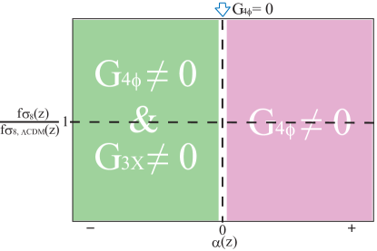
Modified gravity theories, in general, have too many degrees of freedom to be completely analyzed. Consequently, the observables of perturbation quantities (e.g. growth rate of the matter density perturbation) have been investigated only for simple models or for phenomenologically parametrized models. Moreover, the background evolution in modified gravity models is often assumed to be the same as that in the CDM model. In this paper we take account of both the variations of background dynamics and those of perturbation quantities. For this purpose, we introduce new phase diagrams; the and diagrams. Similar diagrams can be found in Refs. [51, 52, 53, 54, 55]. Here describes the effect on gravitational lensing and is defined in Eq. (2.4) below in terms of the deflection potential , and in the case of general relativity (e.g., [56, 57, 58, 59, 60, 61]). Thus, these diagrams will enable us to investigate how each of the two key observations of large-scale structures, RSD and gravitational lensing, can constrain a given modified gravity model.
In this paper, we consider Horndeski’s theory, which is a general scalar-tensor theory. We do not adopt phenomenological parameterizations which have been commonly used in the literature. We focus several specific examples of Horndeski’s gravity and demonstrate how deviations from the CDM model appear in the and diagrams.
The contents of the paper are as follows. We briefly overview how models of dark energy and modified gravity behave on the and diagrams in Sec. 2. For this purpose we present the former and latter diagrams for the simple representative cases of dark energy and modified gravity, the CDM and gravity models, respectively. Then we describe Horndeski’s theory in Sec. 3, and considering its typical examples, we present their and diagrams in Sec. 4. Our concluding remarks are given in Sec. 5. A more detailed description of Horndeski’s theory is presented in Appendix A. A short note on the possibility of having negative is given in Appendix B.
Throughout this paper, we adopt Natural units, , and the gravitational constant is denoted by with the Planck mass of GeV.
2 Dark energy and modified gravity
In models in which dark energy is given by a matter field, commonly its energy momentum tensor is decoupled from the other matter components. In this case, the main effect of dark energy is to modify the background evolution of the Universe, and hence its effect to the growth of linear perturbations is indirect. On the other hand, in modified gravity theories of dark energy, its effective energy momentum tensor is likely to be coupled to the matter components. As a result, not only the background evolution of the Universe but also the linear perturbation equations may significantly deviate from those in the CDM model.
In the following, we assume the metric,
| (2.1) |
and adopt notations in Fourier space as
| (2.2) | |||
| (2.3) |
where is the wave number, is the growing mode of the matter density perturbation, and describes the scale dependence of at initial time under the normalization of as .
In Eq. (2.2), we introduced a quantity , which vanishes in Einstein gravity (i.e., ). The relation of with the well-known gravitational slip parameter, [39], is . Thus characterizes how much a given gravity model deviates from General Relativity (GR). Because the strength of gravitational lensing is determined by the deflection potential [62],
| (2.4) |
we see that the gravitational lensing effect is reduced if or and enhanced if . We note that there is a subtlety in this interpretation. It will be shown in section 4 that, for a class of modified gravity models considered in this paper, the lensing effect is unaffected if we compare it for the same mass distribution.
To see this, let us first introduce which relates the Newton potential to the matter density perturbation in modified gravity:
| (2.5) |
Let us also introduce that would relate the deflection potential to ,
| (2.6) |
We have and in GR. On the other hand, for modified gravity, the -dependence of is found in section 4 as
| (2.7) |
From Eqs. (2.4) and (2.5), we find
| (2.8) |
Hence we obtain
| (2.9) |
Inserting Eq. (2.7) into the above gives , that is, the resulting will be the same as that in GR, independent of .
However, as the mass distribution is measured by its gravitational effect that includes the modification in the effective gravitational constant, what can be compared is the lensing effect for the same . This means our original interpretation is correct from an observational point of view. More precisely speaking, it is the gravitationally inferred mass distribution that is overestimated if or and otherwise if , while the gravitational lensing effect remains the same.
To quantify the growth of linear perturbations, one usually considers the combination, , inferred from galaxy surveys, where and is the normalization parameter of the density perturbation spectrum. In the following, to test modified gravity models, we evaluate the ratio of in a given model to that in the CDM model, . Note that the value of should approach unity in any viable model of gravity in the high-redshift limit. We also assume that the value of coincides with that of the CDM model in the high redshift limit. Thus, this ratio becomes unity at high redshifts. Since depends not only on the modifications of the linear perturbation equations but also on the background evolution of the Universe, below we will study correlations between and and between and the Hubble expansion rate in various models of gravity. The evolution equation of the quasi-static mode of the matter density contrast is expressed as [63, 61]
| (2.10) |
The parameter will be evaluated by using Eq. (2.10) with appropriate initial conditions.
Before presenting detailed studies on modified gravity models, let us first consider the simplest dark energy model, i.e. the CDM model. Note that because there is no deviation from GR in this model. The diagram is depicted in Fig. 2. The initial conditions are set at where they coincides with those of the CDM model. The figure shows that the deviation in is almost proportional to that in the Hubble rate at each redshift, with negative proportionality coefficients. Thus in CDM models becomes smaller than that in the CDM model for models with a larger Hubble rate which corresponds to . We note that the linear perturbation equations in the CDM model are unchanged from those of the CDM model. Therefore, the smaller value of due to a larger may be regarded as a purely background effect. We should note that if we apply a different boundary condition, e.g., and at , the quantitative results will be different though the qualitative tendency will remain the same.


As we mentioned in the above, the behavior of the matter density perturbation is not independent from the background evolution of the Universe in general. In some theories, e.g. gravity theories, even if the difference between the model and GR at the background level is negligibly small, there can be difference at perturbation level due to the scale dependence of the matter density perturbation that enhances the deviation from GR on small scales. As a characteristic example for such a case, let us consider gravity with
| (2.11) |
where and are the current values of the Ricci scalar and the cosmological constant, respectively. For the parameter in the range , this model is known to reproduce the background evolution of the CDM model almost exactly [64]. In Fig. 2, we plot the predicted values of and for several redshifts. In general, the function is not separable, in the other words, the -dependence of in (2.3) cannot be ignored in gravity theories. Here, for definiteness, we plot , i.e. at Mpc. It shows that the density perturbation in this model always evolves faster than that in the case of the CDM model, and is always positive.
3 More general modified gravity models
In the previous section, we studied two examples; CDM model and gravity theory. In the CDM case, the linear perturbation equations are the same as those in the CDM model, while the background evolution of the Universe is different. On the other hand, in the gravity case, the background evolution of the Universe is the same as the CDM model, while the linear perturbation equations are different. In more general modified gravity theories, both of them will be different from the CDM model. Here we consider Horndeski’s theory. It is a general scalar-tensor theory which includes gravity as a special case [63, 65, 66].
The action in Horndeski’s theory is given by [26, 67, 68]
| (3.1) |
where
| (3.2) | ||||
| (3.3) | ||||
| (3.4) | ||||
| (3.5) |
Here, , , , and are generic functions of and , and the subscript means a derivative with respect to . The total action is the sum of and the matter action which contains baryons and cold dark matter. More details are referred to Appendix A
The recent observations of gravitational wave event GW170817 [69] and its electromagnetic counterparts [70, 71, 72] showed that the propagation speed of gravitational waves should satisfy
| (3.6) |
in the relatively recent Universe. This bound implies the sound speed of the tensor mode, given by
| (3.7) |
should be almost unity, where and below the subscript means a derivative with respect to . If the terms , , are relevant for the evolution of the Universe, then one expects a substantial deviation of from unity. Therefore, it is reasonable to assume that the terms proportional to , , and are not relevant for the current accelerated expansion of the Universe. Hence we set in the following.
Even after this simplification, the theory still remains quite complicated. For example, the effective Newton constant that can be defined on sufficiently small scales takes the form [61],
| (3.8) | |||||
| (3.9) | |||||
| (3.10) |
where we have introduced an effective coefficient of the kinetic term
| (3.11) |
As for which describes the modification of the lensing effect, it is expressed using Eq. (3.11) as [61]
| (3.12) |
The above equation shows that is non-vanishing only if is non-trivial, i.e. is -dependent. It also shows that is realized only if provided that we have and which are satisfied for most healthy theories of gravity (see Fig. 3). Thus if , if and , while can be positive or negative if and .
In passing we note that gravity theories correspond to the case [63, 65, 66];
| (3.13) |
Because , is always positive in gravity with . We should note that terms in Eqs. (3.8) and (3.12) are to be taken into account in F(R) gravity models [63]. The case with or may be also acceptable if instabilities are absent. Such a case is discussed in Appendix B, but we will not consider it in the main text for simplicity.
4 Specific examples
Let us now consider a few specific examples of Horndeski’s gravity that show small but observationally interesting deviations from the CDM model. To compare with the CDM model, we will assume the same amount of matter as that in the CDM model, i.e. is fixed, and fix the ratio at sufficiently high redshifts, . In what follows, to evaluate the effects of functions , , and , we assume their forms as
| (4.1) | |||||
| (4.2) | |||||
| (4.3) |
where , , , , and are constant parameters.
In this above class of models, the expressions for and are greatly simplified as
| (4.4) | ||||
| (4.5) |
where defined in Eq. (3.11) is also simplified as
| (4.6) |
As should be small enough to guarantee the proximity to Newton gravity in the large scale structure formation, the above two equations imply that is small and positive if and , and .
Now we are in a position to evaluate the effect of on gravitational lensing for the same mass density distribution. Since the resulting gravitational potential is proportional to the effective gravitational constant , the resulting gravitational lensing effect is proportional to the deflection potential given by
| (4.7) |
where is the gravitational potential of the mass distribution if gravity were GR. Using Eqs. (4.4) and (4.5), we find
| (4.8) |
which gives
| (4.9) |
where is the deflection potential in the case of GR. Thus we see that the gravitational lensing effect is independent of for the same mass density distribution. In particular, it remains essentially the same as that in GR if , as we mentioned in section 2.
4.1 Linear potential, minimally coupled with gravity

First we consider the case with and , which represents a quintessential field [14]. In this case, always vanishes as seen from Eq. (3.12). Figure 4 shows the correlations between and for various values of at several different redshifts. One sees that a higher Hubble rate is accompanied with a lower growth rate of the matter density perturbation, which is similar to the case of the CDM model shown in Fig. 2. Note that also in the CDM model. These similarities are due to the fact that both models have no non-minimal coupling with gravity.
4.2 Flat potential, non-minimally coupled with gravity


Next we consider the effect of non-minimal coupling with gravity, namely, the case where with and (e.g., see [73, 74]). Figure 5 shows the correlations between and and between and . The diagram on the left is similar to that of the minimally coupled linear potential case except for the inclinations of the fitted curves. On the other hand, the diagram is quite different: is always non-negative as in the case of gravity, see Fig. 2 while it vanishes in the minimally coupled linear potential case. We also note that the ratio can be greater or smaller than unity depending on the sign of in contrast to the gravity case where the ratio is always greater than unity. The similarity and difference from the gravity case can be explained by the fact that does not depend on the sign of or , while may increase or decrease depending on the sign of .
4.3 Quadratic potential, non-minimally coupled gravity

The third case we consider is the model which can explain the reconstructed equation-of-state parameter from recent observations [75]. The Lagrangian of the model is given by
| (4.10) |
This model is similar to a combination of the models considered in subsections 4.1 and 4.2. However, it differs from such a model in that there is an oscillation of the equation of state parameter induced by the oscillation of the scalar field, which gives rise to an oscillatory evolution in the Hubble rate as can be seen in the left panel of Fig. 6. We find in this model is always smaller than that in the CDM model even at at which . This result may be understood if we note the fact that , which is proportional to, depends non-locally on time, or it is a hysteresis effect of the oscillatory evolution in the present case. We also note that does not vary much within the range of parameters we adopted, with the values in the range .
Actually the small positiveness of is a common feature in models that satisfy and , provided that the background evolution does not deviate much from that in the CDM model. This may be seen by comparing Eqs. (4.4) and (4.5). If we require to be small enough to guarantee the proximity to Newton gravity, namely, , these two equations implies that is small and positive if and .
4.4 Non-canonical kinetic term


If we want to consider models with larger values of and possibly substantial deviations of from Newton gravity, we need to relax the assumption . From Eq. (3.12), one notices that can be realized if . Since and for a canonical scalar field, one has to resort to a non-canonical scalar field model to achieve it. For definiteness, we propose the following model,
| (4.11) |
which gives . For , for a slowly rolling scalar field. Thus this model can achieve and hence . Here we focus on the case because the scalar field would become non-dynamical if and it would become a ghost if .
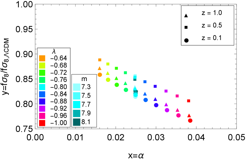
Figure 7 shows the and diagrams in this case for various values of in units of . As seen from the left panel, the background evolution of the Universe is almost same as that in the CDM, with . This behavior is similar to gravity. The right figure shows that is certainly realized in this case. means that the gravitational lensing effect is enhanced by a factor . We note that, for a more general form of , we may achieve any value of in the range while keeping the CDM like background evolution intact. We also note that would substantially deviate from the Newtonian if as seen from Eq. (4.8).
The initial value of the scalar field is chosen rather arbitrarily, except for the model discussed in Sec. 4.3, but in a way that it can exhibit characteristic, qualitative features of each model. For example, in the case of the model considered in Sec. 4.1, the tendency shown in Fig. 4 remains the same for other choices of the initial conditions. As for Sec. 4.3, the initial condition is chosen so that it reproduces the observationally constrained/indicated evolution of . One may worry about the validity of the small scale approximation because some of modified gravity theories have strong dependence on the wave number . In fact, the matter density perturbation can strongly depend on the scale in Horndeski’s theory if there is a hierarchy between , , and or if there is a hierarchy between their derivatives. In the case of gravity, should be satisfied to accord with observations and these conditions cause the scale dependence of the matter density perturbation. The reason why the scale dependence appears is that there are two limits [76]: and . The Compton wavelength is determined by balancing these two conditions, then the condition is superior to inside the Compton wavelength. The cases we considered in this section do not have such a hierarchy, therefore, the small scale approximation is always valid if we focus on a scale which is deep inside the horizon.
5 Conclusion
We have investigated a class of dark energy models based on Horndeski’s theory of modified gravity which exhibit small but interesting deviations from the CDM model not only in the background evolution but also in the linear perturbation level. The models include the CDM, gravity, and four kinds of Horndeski gravity models. To classify the properties of these models, we have introduced two diagrams; and diagrams. We have found that these two diagrams provide a useful tool to distinguish the differences in the observational predictions of different models from each other.

Figure 8 shows the summary of our results. The right panel shows the diagram, which exhibits deviations in the behavior of linear perturbations from GR, at for various models with various parameters. The canonical scalar model with linear potential (denoted by V1, discussed in section 4.1) does not have a direct coupling to gravity, hence . The non-minimally coupled scalar model with flat potential (denoted by G4, discussed in section 4.2) gives non-vanishing but the values are too small () to be seen in the figure, whereas the non-minimally coupled scalar model with quadratic potential (denoted by G4m2, discussed in section 4.3) . As for the non-minimally coupled scalar model with non-canonical kinetic term (denoted by G4Kx, discussed in section 4.4), , that is the dynamics of the linear perturbation is quite different from GR.
In all of the models studied in this paper, we have found . As discussed in Appendix B, there exist theoretically acceptable models with negative , but they all satisfy . In fact, the condition is necessary to guarantee the positivity of as can be seen from Eq. (4.8). Thus either or , our result implies that gravity becomes effectively stronger than GR in all the models. In other words, if we are to measure the mass density distribution, we would overestimate it if we use the gravitational dynamics, while we would obtain a correct estimate if we use gravitational lensing observations. Whether this has any substantial implications to observational data analysis is an issue to be studied.
The left panel shows the diagram at for various models with various parameters. It shows the dependence of the growth rate of linear perturbations on the difference in the background evolution of the Universe. We see that in all models except for the non-minimally coupled scalar model with quadratic potential or non-canonical kinetic term, there is a tendency that larger gives smaller in comparison with CDM. In the case of the quadratic potential model (G4m2), because of the oscillatory feature in , the fact that are smaller for smaller depends on the redshift, as well as on the choice of the model parameters. So it is difficult to discuss a general tendency in this model. In the case of the non-canonical kinetic term model (G4Kx), the dependence of on seems very small. This is explained by the fact that this model can mimic the CDM model very well as long as the background evolution of the Universe is concerned.
The cosmic shear power spectrum in weak lensing surveys and the redshift-space power spectrum in galaxy surveys directly constrain and , respectively. The latter observable can further probe using BAO as a standard ruler. The blue bars denote observational error bars obtained by Alam [77]. Since it is a constraint, no reliable conclusion can be drawn, but it seems that when compared to the CDM model, those models that yield slightly larger with slightly smaller are preferred. It is, however, important to note that most of the current observational analyses have been performed assuming CDM and GR, a so-called consistency test. In order to test a modified gravity model, one needs to use a theoretical template of the power spectrum with the given gravity model [78, 79, 47]. Ref. [80] has derived an analytic formula of the matter power spectrum in real space under Horndeski’s theory. Further theoretical efforts are required in order to constrain general modified gravity models on the diagrams proposed in this paper.
So far, observational constraints are not so severe yet to exclude any of these models. But eventually we will be able to exclude most of the models as observational accuracies improve. The and diagrams we introduced, or their variants, may play an important role at such a stage.
Acknowledgments
We would like to thank T. Namikawa for discussions in the early stage of this work. T. O. acknowledges support from the Ministry of Science and Technology of Taiwan under Grants No. MOST 106-2119-M-001-031-MY3 and the Career Development Award, Academia Sinina (AS-CDA-108-M02) for the period of 2019 to 2023. The work of M. S. is supported in part by JSPS KAKENHI No. 20H04727.
Appendix A Horndeski’s theory
Let us first recapitulate the action in Horndeski’s theory [26, 67, 68],
| (A.1) |
where
| (A.2) | ||||
| (A.3) | ||||
| (A.4) | ||||
| (A.5) |
Here, , , , and are generic functions of and , and the subscript means a derivative with respect to . The total action is the sum of and the matter action .
The Friedman equations are given by [68]
| (A.6) |
where
| (A.7) | ||||
| (A.8) | ||||
| (A.9) | ||||
| (A.10) |
and
| (A.11) |
where
| (A.12) | ||||
| (A.13) | ||||
| (A.14) | ||||
| (A.15) |
Here, is the Hubble rate function and the dot means derivative with respect to time and and are the matter energy density and the pressure, respectively. The equation of motion of the scalar field is given by varying the action with respect to :
| (A.16) |
where
| (A.17) |
| (A.18) |
Equations (A.6), (A.11), and (A.16) control the background evolution of the Universe. In the same manner as the quintessence model, Eqs. (A.11) and (A.16) are equivalent when Eq. (A.6) holds. Equations (A.6) and (A.11) can be rewritten in the well-known form
| (A.19) | |||
| (A.20) |
where we defined and as
| (A.21) |
These equations define the effective energy density and effective pressure, respectively. As for the matter part, we may set as the pressures of both baryons and cold dark matter are negligible.
Appendix B Possibility of
As mentioned in Sec. 4, a negative can be realized in the case and . To see this, we recapitulate the expression for ,
| (B.1) |
Hence we have if we consider a model with , which may be realized by making the same order of . A simplest model would be to set and with . But we have not checked if this model could give an observationally viable model or not.
Another possibility is to consider . In this case it seems there are many ways to realize a negative . Here let us consider the case . In this case, we should take care of no ghost and no gradient instability conditions. No ghost condition and the condition are expressed as [75, 81]
| (B.2) | |||
| (B.3) |
where is assumed to prevent the instability in the tensor perturbation.
A simple example to realize a negative without instabilities is the case , , , and . In this case, the stability conditions (B.2) and (B.3) are expressed by a single equation;
| (B.4) |
which is re-expressed as
| (B.5) |
The expressions for and are given by
| (B.6) | ||||
| (B.7) |
We note that this gives the same expression for as the one obtained for the models discussed in section 4 when expressed in terms of ,
| (B.8) |
The stability condition (B.5) implies that may take the value in the range, and . The stability also guarantees the positivity of .. A negative can be realized for . Both for negative and positive values of , the effective gravitational force becomes twice as strong as GR in the limit of large .
References
- [1] A. G. Riess, A. V. Filippenko, P. Challis, A. Clocchiatti, A. Diercks, P. M. Garnavich et al., Observational Evidence from Supernovae for an Accelerating Universe and a Cosmological Constant, Astron. J. 116 (1998) 1009 [astro-ph/9805201].
- [2] S. Perlmutter, G. Aldering, G. Goldhaber, R. A. Knop, P. Nugent, P. G. Castro et al., Measurements of and from 42 High-Redshift Supernovae, Astrophys. J. 517 (1999) 565 [astro-ph/9812133].
- [3] E. Komatsu, K. M. Smith, J. Dunkley, C. L. Bennett, B. Gold, G. Hinshaw et al., Seven-year Wilkinson Microwave Anisotropy Probe (WMAP) Observations: Cosmological Interpretation, Astrophys. J. Suppl. 192 (2011) 18 [1001.4538].
- [4] Planck Collaboration, P. A. R. Ade, N. Aghanim, C. Armitage-Caplan, M. Arnaud, M. Ashdown et al., Planck 2013 results. XVI. Cosmological parameters, Astron. Astrophys. 571 (2014) A16 [1303.5076].
- [5] Planck Collaboration, P. A. R. Ade, N. Aghanim, M. Arnaud, M. Ashdown, J. Aumont et al., Planck 2015 results. XIII. Cosmological parameters, Astron. Astrophys. 594 (2016) A13 [1502.01589].
- [6] D. J. Eisenstein, I. Zehavi, D. W. Hogg, R. Scoccimarro, M. R. Blanton, R. C. Nichol et al., Detection of the Baryon Acoustic Peak in the Large-Scale Correlation Function of SDSS Luminous Red Galaxies, Astrophys. J. 633 (2005) 560 [arXiv:astro-ph/0501171].
- [7] T. Okumura, T. Matsubara, D. J. Eisenstein, I. Kayo, C. Hikage, A. S. Szalay et al., Large-Scale Anisotropic Correlation Function of SDSS Luminous Red Galaxies, Astrophys. J. 676 (2008) 889 [0711.3640].
- [8] W. J. Percival, B. A. Reid, D. J. Eisenstein, N. A. Bahcall, T. Budavari, J. A. Frieman et al., Baryon acoustic oscillations in the Sloan Digital Sky Survey Data Release 7 galaxy sample, Mon. Not. Roy. Astron. Soc. 401 (2010) 2148 [0907.1660].
- [9] C. Blake, E. A. Kazin, F. Beutler, T. M. Davis, D. Parkinson, S. Brough et al., The WiggleZ Dark Energy Survey: mapping the distance-redshift relation with baryon acoustic oscillations, Mon. Not. Roy. Astron. Soc. 418 (2011) 1707 [1108.2635].
- [10] F. Beutler, C. Blake, M. Colless, D. H. Jones, L. Staveley-Smith, L. Campbell et al., The 6dF Galaxy Survey: baryon acoustic oscillations and the local Hubble constant, Mon. Not. Roy. Astron. Soc. 416 (2011) 3017 [1106.3366].
- [11] A. J. Cuesta, M. Vargas-Magaña, F. Beutler, A. S. Bolton, J. R. Brownstein, D. J. Eisenstein et al., The clustering of galaxies in the SDSS-III Baryon Oscillation Spectroscopic Survey: baryon acoustic oscillations in the correlation function of LOWZ and CMASS galaxies in Data Release 12, Mon. Not. Roy. Astron. Soc. 457 (2016) 1770 [1509.06371].
- [12] T. Delubac, J. E. Bautista, N. G. Busca, J. Rich, D. Kirkby, S. Bailey et al., Baryon acoustic oscillations in the Ly forest of BOSS DR11 quasars, Astron. Astrophys. 574 (2015) A59 [1404.1801].
- [13] P. J. E. Peebles and B. Ratra, Cosmology with a Time-Variable Cosmological “Constant”, Astrophys. J. Let. 325 (1988) L17.
- [14] B. Ratra and P. J. E. Peebles, Cosmological consequences of a rolling homogeneous scalar field, Phys. Rev. D 37 (1988) 3406.
- [15] T. Chiba, N. Sugiyama and T. Nakamura, Cosmology with x-matter, Mon. Not. Roy. Astron. Soc. 289 (1997) L5 [astro-ph/9704199].
- [16] I. Zlatev, L. Wang and P. J. Steinhardt, Quintessence, Cosmic Coincidence, and the Cosmological Constant, Phys. Rev. Lett. 82 (1999) 896 [astro-ph/9807002].
- [17] H. A. Buchdahl, Non-linear Lagrangians and cosmological theory, Mon. Not. Roy. Astron. Soc. 150 (1970) 1.
- [18] S. Nojiri and S. D. Odintsov, Introduction to Modified Gravity and Gravitational Alternative for Dark Energy, arXiv e-prints (2006) hep [hep-th/0601213].
- [19] T. P. Sotiriou and V. Faraoni, f(R) theories of gravity, Reviews of Modern Physics 82 (2010) 451 [0805.1726].
- [20] A. De Felice and S. Tsujikawa, f( R) Theories, Living Reviews in Relativity 13 (2010) 3 [1002.4928].
- [21] S. Nojiri and S. D. Odintsov, Unified cosmic history in modified gravity: From F(R) theory to Lorentz non-invariant models, Phys. Rept. 505 (2011) 59 [1011.0544].
- [22] S. Nojiri, S. D. Odintsov and V. K. Oikonomou, Modified gravity theories on a nutshell: Inflation, bounce and late-time evolution, Phys. Rept. 692 (2017) 1 [1705.11098].
- [23] C. de Rham, G. Gabadadze and A. J. Tolley, Resummation of Massive Gravity, Phys. Rev. Lett. 106 (2011) 231101 [1011.1232].
- [24] S. F. Hassan and R. A. Rosen, Resolving the Ghost Problem in Nonlinear Massive Gravity, Phys. Rev. Lett. 108 (2012) 041101 [1106.3344].
- [25] S. F. Hassan and R. A. Rosen, Bimetric gravity from ghost-free massive gravity, Journal of High Energy Physics 02 (2012) 126 [1109.3515].
- [26] G. W. Horndeski, Second-Order Scalar-Tensor Field Equations in a Four-Dimensional Space, International Journal of Theoretical Physics 10 (1974) 363.
- [27] V. Marra, L. Amendola, I. Sawicki and W. Valkenburg, Cosmic Variance and the Measurement of the Local Hubble Parameter, Phys. Rev. Lett. 110 (2013) 241305 [1303.3121].
- [28] A. G. Riess, L. M. Macri, S. L. Hoffmann, D. Scolnic, S. Casertano, A. V. Filippenko et al., A 2.4% Determination of the Local Value of the Hubble Constant, Astrophys. J. 826 (2016) 56 [1604.01424].
- [29] E. Di Valentino, A. Melchiorri and J. Silk, Reconciling Planck with the local value of H0 in extended parameter space, Physics Letters B 761 (2016) 242 [1606.00634].
- [30] K. C. Wong, S. H. Suyu, G. C. F. Chen, C. E. Rusu, M. Millon, D. Sluse et al., H0LiCOW XIII. A 2.4% measurement of from lensed quasars: tension between early and late-Universe probes, arXiv e-prints (2019) arXiv:1907.04869 [1907.04869].
- [31] G. C. F. Chen, C. D. Fassnacht, S. H. Suyu, C. E. Rusu, J. H. H. Chan, K. C. Wong et al., A SHARP view of H0LiCOW: H0 from three time-delay gravitational lens systems with adaptive optics imaging, Mon. Not. Roy. Astron. Soc. 490 (2019) 1743 [1907.02533].
- [32] S. Birrer, T. Treu, C. E. Rusu, V. Bonvin, C. D. Fassnacht, J. H. H. Chan et al., H0LiCOW - IX. Cosmographic analysis of the doubly imaged quasar SDSS 1206+4332 and a new measurement of the Hubble constant, Mon. Not. Roy. Astron. Soc. 484 (2019) 4726 [1809.01274].
- [33] I. Jee, S. H. Suyu, E. Komatsu, C. D. Fassnacht, S. Hilbert and L. V. E. Koopmans, A measurement of the Hubble constant from angular diameter distances to two gravitational lenses, Science 365 (2019) 1134 [1909.06712].
- [34] A. J. Shajib, S. Birrer, T. Treu, A. Agnello, E. J. Buckley-Geer, J. H. H. Chan et al., STRIDES: A 3.9 per cent measurement of the Hubble constant from the strong lens system DES J0408-5354, Mon. Not. Roy. Astron. Soc. (2020) [1910.06306].
- [35] L. Verde, T. Treu and A. G. Riess, Tensions between the early and late Universe, Nature Astronomy 3 (2019) 891 [1907.10625].
- [36] N. Kaiser, Clustering in real space and in redshift space, Mon. Not. Roy. Astron. Soc. 227 (1987) 1.
- [37] A. J. S. Hamilton, Linear Redshift Distortions: a Review, in The Evolving Universe, D. Hamilton, ed., vol. 231 of Astrophysics and Space Science Library, p. 185, (1998), DOI.
- [38] E. V. Linder, Cosmic growth history and expansion history, Phys. Rev. D 72 (2005) 043529 [arXiv:astro-ph/0507263].
- [39] B. Jain and P. Zhang, Observational tests of modified gravity, Phys. Rev. D 78 (2008) 063503 [0709.2375].
- [40] L. Guzzo, M. Pierleoni, B. Meneux, E. Branchini, O. Le Fèvre, C. Marinoni et al., A test of the nature of cosmic acceleration using galaxy redshift distortions, Nature 451 (2008) 541 [0802.1944].
- [41] Y.-S. Song and K. Koyama, Consistency test of general relativity from large scale structure of the universe, JCAP 1 (2009) 48 [0802.3897].
- [42] T. Okumura and Y. P. Jing, Systematic Effects on Determination of the Growth Factor from Redshift-space Distortions, Astrophys. J. 726 (2011) 5 [1004.3548].
- [43] C. Blake, S. Brough, M. Colless, C. Contreras, W. Couch, S. Croom et al., The WiggleZ Dark Energy Survey: the growth rate of cosmic structure since redshift z=0.9, Mon. Not. Roy. Astron. Soc. (2011) 834 [1104.2948].
- [44] L. Samushia, W. J. Percival and A. Raccanelli, Interpreting large-scale redshift-space distortion measurements, Mon. Not. Roy. Astron. Soc. 420 (2012) 2102 [1102.1014].
- [45] S. de la Torre, L. Guzzo, J. A. Peacock, E. Branchini, A. Iovino, B. R. Granett et al., The VIMOS Public Extragalactic Redshift Survey (VIPERS) . Galaxy clustering and redshift-space distortions at in the first data release, Astron. Astrophys. 557 (2013) A54 [1303.2622].
- [46] B. A. Reid, H.-J. Seo, A. Leauthaud, J. L. Tinker and M. White, A 2.5 per cent measurement of the growth rate from small-scale redshift space clustering of SDSS-III CMASS galaxies, Mon. Not. Roy. Astron. Soc. 444 (2014) 476 [1404.3742].
- [47] Y.-S. Song, A. Taruya, E. Linder, K. Koyama, C. G. Sabiu, G.-B. Zhao et al., Consistent modified gravity analysis of anisotropic galaxy clustering using BOSS DR11, Phys. Rev. D 92 (2015) 043522 [1507.01592].
- [48] T. Okumura, C. Hikage, T. Totani, M. Tonegawa, H. Okada, K. Glazebrook et al., The Subaru FMOS galaxy redshift survey (FastSound). IV. New constraint on gravity theory from redshift space distortions at , Publ. Astron. Soc. Japan 68 (2016) 38 [1511.08083].
- [49] L. Kazantzidis and L. Perivolaropoulos, Evolution of the f 8 tension with the Planck15 / CDM determination and implications for modified gravity theories, Phys. Rev. D 97 (2018) 103503 [1803.01337].
- [50] S. Nesseris, G. Pantazis and L. r. Perivolaropoulos, Tension and constraints on modified gravity parametrizations of Geff(z ) from growth rate and Planck data, Phys. Rev. D 96 (2017) 023542 [1703.10538].
- [51] L. Perenon, C. Marinoni and F. Piazza, Diagnostic of Horndeski theories, JCAP 1 (2017) 035 [1609.09197].
- [52] E. V. Linder, Cosmic growth and expansion conjoined, Astroparticle Physics 86 (2017) 41 [1610.05321].
- [53] S. Basilakos and S. Nesseris, Conjoined constraints on modified gravity from the expansion history and cosmic growth, Phys. Rev. D 96 (2017) 063517 [1705.08797].
- [54] E. V. Linder, No slip gravity, JCAP 3 (2018) 005 [1801.01503].
- [55] E. V. Linder, No Run Gravity, JCAP 7 (2019) 034 [1903.02010].
- [56] K. Koyama, Structure formation in modified gravity models, JCAP 3 (2006) 017 [astro-ph/0601220].
- [57] S. A. Thomas, F. B. Abdalla and J. Weller, Constraining modified gravity and growth with weak lensing, Mon. Not. Roy. Astron. Soc. 395 (2009) 197 [0810.4863].
- [58] S. F. Daniel, E. V. Linder, T. L. Smith, R. R. Caldwell, A. Cooray, A. Leauthaud et al., Testing general relativity with current cosmological data, Phys. Rev. D 81 (2010) 123508 [1002.1962].
- [59] I. Tereno, E. Semboloni and T. Schrabback, COSMOS weak-lensing constraints on modified gravity, Astron. Astrophys. 530 (2011) A68 [1012.5854].
- [60] F. Simpson, C. Heymans, D. Parkinson, C. Blake, M. Kilbinger, J. Benjamin et al., CFHTLenS: testing the laws of gravity with tomographic weak lensing and redshift-space distortions, Mon. Not. Roy. Astron. Soc. 429 (2013) 2249 [1212.3339].
- [61] J. Matsumoto, Oscillating solutions of the matter density contrast in Horndeski’s theory, JCAP 1 (2019) 054 [1806.10454].
- [62] C. Schimd, J.-P. Uzan and A. Riazuelo, Weak lensing in scalar-tensor theories of gravity, Phys. Rev. D 71 (2005) 083512 [astro-ph/0412120].
- [63] A. de Felice, T. Kobayashi and S. Tsujikawa, Effective gravitational couplings for cosmological perturbations in the most general scalar-tensor theories with second-order field equations, Physics Letters B 706 (2011) 123 [1108.4242].
- [64] W. Hu and I. Sawicki, Models of f(R) cosmic acceleration that evade solar system tests, Phys. Rev. D 76 (2007) 064004 [0705.1158].
- [65] J. O’Hanlon, Intermediate-Range Gravity: A Generally Covariant Model, Phys. Rev. Lett. 29 (1972) 137.
- [66] T. Chiba, 1/R gravity and scalar-tensor gravity, Physics Letters B 575 (2003) 1 [astro-ph/0307338].
- [67] C. Deffayet, X. Gao, D. A. Steer and G. Zahariade, From k-essence to generalized Galileons, Phys. Rev. D 84 (2011) 064039 [1103.3260].
- [68] T. Kobayashi, M. Yamaguchi and J. Yokoyama, Generalized G-Inflation — Inflation with the Most General Second-Order Field Equations —, Progress of Theoretical Physics 126 (2011) 511 [1105.5723].
- [69] B. P. Abbott, R. Abbott, T. D. Abbott, F. Acernese, K. Ackley, C. Adams et al., GW170817: Observation of Gravitational Waves from a Binary Neutron Star Inspiral, Phys. Rev. Lett. 119 (2017) 161101 [1710.05832].
- [70] B. P. Abbott, R. Abbott, T. D. Abbott, F. Acernese, K. Ackley, C. Adams et al., Gravitational Waves and Gamma-Rays from a Binary Neutron Star Merger: GW170817 and GRB 170817A, Astrophys. J. Let. 848 (2017) L13 [1710.05834].
- [71] B. P. Abbott, R. Abbott, T. D. Abbott, F. Acernese, K. Ackley, C. Adams et al., Multi-messenger Observations of a Binary Neutron Star Merger, Astrophys. J. Let. 848 (2017) L12 [1710.05833].
- [72] D. A. Coulter, R. J. Foley, C. D. Kilpatrick, M. R. Drout, A. L. Piro, B. J. Shappee et al., Swope Supernova Survey 2017a (SSS17a), the optical counterpart to a gravitational wave source, Science 358 (2017) 1556 [1710.05452].
- [73] C. Brans and R. H. Dicke, Mach’s Principle and a Relativistic Theory of Gravitation, Physical Review 124 (1961) 925.
- [74] Y. Fujii and K.-I. Maeda, The Scalar-Tensor Theory of Gravitation. 2003.
- [75] J. Matsumoto, Phantom crossing dark energy in Horndeski’s theory, Phys. Rev. D 97 (2018) 123538 [1712.10015].
- [76] J. Matsumoto, Cosmological perturbations in F(R) gravity, Phys. Rev. D 87 (2013) 104002 [1303.6828].
- [77] S. Alam, M. Ata, S. Bailey, F. Beutler, D. Bizyaev, J. A. Blazek et al., The clustering of galaxies in the completed SDSS-III Baryon Oscillation Spectroscopic Survey: cosmological analysis of the DR12 galaxy sample, ArXiv e-prints (2016) [1607.03155].
- [78] K. Koyama, A. Taruya and T. Hiramatsu, Nonlinear evolution of the matter power spectrum in modified theories of gravity, Phys. Rev. D 79 (2009) 123512 [0902.0618].
- [79] A. Taruya, T. Nishimichi, F. Bernardeau, T. Hiramatsu and K. Koyama, Regularized cosmological power spectrum and correlation function in modified gravity models, Phys. Rev. D 90 (2014) 123515 [1408.4232].
- [80] Y. Takushima, A. Terukina and K. Yamamoto, Bispectrum of cosmological density perturbations in the most general second-order scalar-tensor theory, Phys. Rev. D 89 (2014) 104007 [1311.0281].
- [81] A. De Felice and S. Tsujikawa, Conditions for the cosmological viability of the most general scalar-tensor theories and their applications to extended Galileon dark energy models, JCAP 2 (2012) 7 [1110.3878].