\rmfcaptionstyle

New insight in the 2-flavor Schwinger model based on lattice simulations

Jaime Fabián Nieto Castellanos Wolfgang Bietenholz Instituto de Ciencias Nucleares, Universidad Nacional Autónoma de México
A.P. 70-543, C.P. 04510 Ciudad de México, Mexico Ivan Hip Faculty of Geotechnical Engineering, University of Zagreb
Hallerova aleja 7, 42000 Varaždin, Croatia

Abstract

We consider the Schwinger model with two degenerate, light fermion flavors by means of lattice simulations. At finite temperature, we probe the viability of a bosonization method by Hosotani et al. Next we explore an analogue to the pion decay constant, which agrees for independent formulations based on the Gell-Mann–Oakes–Renner relation, the 2-dimensional Witten–Veneziano formula and the $\delta$ -regime. Finally we confront several conjectures about the chiral condensate with lattice results.

pacs:

11.10.Kk, 11.10.Wx, 11.15.Ha, 12.20.-m

\keys

Schwinger model, lattice gauge theory, finite temperature, chiral condensate, $\delta$ -regime, pion decay constant

1 The 2-flavor Schwinger model

In the early 1960s, when quantum field theory was yet to be elaborated as the correct theory of particle physics, Schwinger [2] analyzed Quantum Electrodynamics in $d=2$ space-time dimensions (QED₂, or Schwinger model). It shares qualitative properties with QCD, in particular confinement, chiral symmetry breaking and topology.

Schwinger was particularly interested in the emergence of mass, which was puzzling before the Higgs mechanism was established. In fact, for $N_{\rm f}$ massless fermion flavors, the spectrum of QED₂ includes one massive and $N_{\rm f}-1$ independent massless bosons. By analogy to QCD we denote them as the “ $\eta$ -meson” (which could also be interpreted as a massive “photon”) and the “pions”. The $\eta$ -mass was computed analytically [3],

m_{\eta}^{2}=\frac{N_{\rm f}g^{2}}{\pi}\ ,

(1)

where $g$ is the gauge coupling.

At a degenerate fermion mass $m>0$ , there are conjectures but no exact solutions for the masses $m_{\pi}$ and $m_{\eta}$ . They can be numerically measured with lattice simulations, which provide fully non-perturbative results. We present such simulation results, which we obtained with $N_{\rm f}=2$ degenerate flavors of dynamical Wilson fermions, using the Hybrid Monte Carlo algorithm. The renormalized fermion mass $m$ was measured based on the PCAC relation. Part of these results were anticipated in Ref. [4].

2 “Meson” masses at finite temperature

Bosonization reduces the Schwinger model to a quantum mechanical system of $N_{\rm f}-1$ degrees of freedom; we call its temporal size $L_{t}$ . In the case of $N_{\rm f}=2$ degenerate flavors of mass $m$ , this method encodes the masses $m_{\pi}$ and $m_{\eta}$ in a Schrödinger-type equation for a periodic function $f(\varphi)=f(\varphi+2\pi)$ [5],

$\displaystyle\epsilon f(\varphi)$	$\displaystyle=$	$\displaystyle\left(-\frac{d^{2}}{d\varphi^{2}}-\kappa\cos\varphi\right)f(\varphi)\ ,$
$\displaystyle\kappa$	$\displaystyle=$	$\displaystyle\frac{4}{\pi}mL_{t}\left[B(m_{\eta}L_{t})B(m_{\pi}L_{t})\right]^{1/2}e^{-\pi/(2\mu L_{t})}\ ,$
$\displaystyle B(z)$	$\displaystyle=$	$\displaystyle\frac{z}{4\pi}\textrm{exp}\left[\gamma+\frac{\pi}{z}-2\int_{1}^{\infty}\frac{du}{(e^{uz}-1)\sqrt{u^{2}-1}}\right]\ ,$
$\displaystyle m_{\pi}^{2}$	$\displaystyle=$	$\displaystyle\frac{2\pi^{2}}{L_{\rm t}^{2}}\kappa\int_{-\pi}^{\pi}d\varphi\ \cos\varphi\ \|f_{0}(\varphi)\|^{2}\ ,$
$\displaystyle m_{\eta}^{2}$	$\displaystyle=$	$\displaystyle m_{\pi}^{2}+\mu^{2}\ ,\quad\mu=\sqrt{\frac{2}{\pi}}\,g\ ,$	(2)

where $\gamma=0.577\dots$ is Euler’s constant, $\epsilon$ is the energy, and $f_{0}$ the ground state function. This system of equations can be solved numerically [6], but the viability of its solution is limited to $m\ll\mu$ .

In an infinite spatial volume, for a small mass $m$ , the solution to eqs. (2) for the “pion” mass takes the form

m_{\pi}=4e^{2\gamma}\sqrt{\frac{2}{\pi}}(m^{2}g)^{1/3}=2.1633\dots(m^{2}g)^{1/3}.

(3)

This is similar to another infinite volume prediction by Smilga [7], $m_{\pi}=2.008\dots(m^{2}g)^{1/3}$ . Figure 1 compares the solution to Hosotani’s equations (2) and the asymptotic formula (3) to our simulation results on a lattice of size $L_{t}\times L=12\times 64$ , at $\beta\equiv 1/g^{2}=4$ (in lattice units), as a function of the fermion mass $m$ .

Refer to caption — Figure 1: The masses $m_{\pi}$ and $m_{\eta}$ , depending on the renormalized fermion mass $m$ . We show results obtained from Hosotani’s equations (2), from the asymptotic formula (3), from light-cone quantization [8], and from lattice simulations.

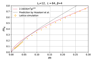
We observe a quasi-chiral regime, with $m\lesssim 0.05$ , where the predictions for $m_{\pi}$ based on Hosotani’s formula is manifestly successful. There is another regime around $0.25\lesssim m\lesssim 0.3$ where the asymptotic formula for $m_{\pi}$ agrees with the lattice data, but that could be accidental, since the slopes differ.

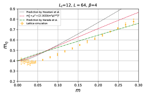
On the other hand, the results for $m_{\eta}$ illustrate that none of the predictions is accurate, except perhaps at tiny fermion mass, where even the simple formula (1) for the chiral limit is more successful (it yields $m_{\eta}=0.3989\dots$ ). In that case, we include a predictions, which is given — up to re-scaling — in Ref. [8], $m_{\eta}=\frac{g}{\sqrt{\pi}}[e^{0.19}(\sqrt{\pi}m/g)^{0.993}+\sqrt{2}],$ and which is (accidentally) close the the lattice data around $m\approx 0.23$ .

3 The “pion decay constant”

A frequent question about the multi-flavor Schwinger model refers to the “pions” in the chiral limit, $m=0$ : they are massless, but in contrast to QCD they cannot represent Nambu-Goldstone bosons due to the Mermin-Wagner-Coleman Theorem — although at small $m>0$ they behave much like quasi-Nambu-Goldstone bosons. An explanation is given e.g. in Ref. [9]: at $m=m_{\pi}=0$ the “pions” do not interact.

Regarding the standard definition of the pion decay constant¹¹1Note that this “pion” does not actually decay. $F_{\pi}$ ,

\langle 0|J_{\mu}^{5}(0)|\pi(p)\rangle={\rm i}p_{\mu}F_{\pi}\ ,

(4)

this property suggests $F_{\pi}(m=0)=0$ .

However, there are other ways to define an analogue to $F_{\pi}$ in the 2-flavor Schwinger model, which lead to finite values. We are going to see that they are quite consistent.

To the best of our knowledge, there is only one non-trivial prediction in the literature for $F_{\pi}$ in the 2-flavor Schwinger model [8]. It is based on a light-cone quantization approach and it refers to the relation

\langle 0|\partial_{\mu}J_{\mu}^{5}(0)|\pi(p)\rangle=m_{\pi}^{2}F_{\pi}\ ,

(5)

which we infer from eq. (4), but this form allows for $F_{\pi}(m=0)>0$ . Harada et al. obtained a very mild dependence on the (degenerate) fermion mass $m$ [8],

F_{\pi}(m)=0.394518(14)+0.040(1)\,\frac{m}{g}\ .

(6)

Note that $F_{\pi}$ is dimensionless in 2 dimensions.

3.1 Gell-Mann–Oakes–Renner relation

The Schwinger model analogue of the Gell-Mann–Oakes–Renner relation reads [10]

F_{\pi}^{2}(m)=\frac{2m\Sigma}{m_{\pi}^{2}}\ ,

(7)

where $\Sigma=-\langle\bar{\psi}\psi\rangle$ is the chiral condensate. Substituting infinite volume and low mass expressions given in Ref. [11],

\Sigma=\frac{1}{\pi}\left(\frac{e^{4\gamma}m\mu^{2}}{4}\right)^{1/3}\ ,\quad m_{\pi}=(4e^{2\gamma}m^{2}\mu)^{1/3}\ ,

(8)

yields

F_{\pi}=\frac{1}{\sqrt{2\pi}}=0.3989\dots\ .

(9)

This result is constant in $m$ and $g$ , but for $m/g=0$ — or close to it — we observe agreement with eq. (6) up to $1\,\%$ . Ref. [11] also provides formulae for $\Sigma$ and $m_{\pi}$ in two other regimes, depending on $m$ and the volume. Inserting either of them consistently leads again to eq. (9). One might also insert the numerically measured values of $m_{\pi}$ and $\Sigma$ , see Section 4; this analysis is in progress.

3.2 The 2d Witten–Veneziano formula

In ’t Hooft’s formulation of large- $N_{\rm c}$ QCD, the Witten–Veneziano formula [12] relates the $\eta^{\prime}$ -mass to the quenched topological susceptibility $\chi_{\rm t}^{\rm q}$ . In particular, it explains — as a topological effect — why the $\eta^{\prime}$ -meson is so heavy compared to the light meson octet. This relation involves the decay constant $F_{\eta^{\prime}}$ , which — at large $N_{\rm c}$ — coincides with $F_{\pi}$ .

According to Ref. [13], the analogous relation in the multi-flavor Schwinger model is actually more robust. In the chiral limit it reads

m_{\eta}^{2}=\frac{2N_{\rm f}}{F_{\eta}^{2}}\chi_{\rm t}^{\rm q}\ .

(10)

If we employ relation (1) along with the formula [14]

\chi_{\rm t}^{\rm q}=\frac{g^{2}}{4\pi}\ ,

(11)

we obtain

F_{\eta}=\frac{1}{\sqrt{2\pi}}\ .

(12)

If we further assume $F_{\eta}=F_{\pi}$ , as in large- $N_{\rm c}$ QCD, we arrive at exact agreement with eq. (9).

Formula (11) is well tested as the continuum limit of various lattice actions [4], as requested by universality, see also Refs. [15]. On the other hand, we are not aware of a sound justification for setting $F_{\eta}=F_{\pi}$ in the Schwinger model.

3.3 The $\delta$ -regime

We proceed to yet another, independent way of introducing an analogue to $F_{\pi}$ . Here we refer to the $\delta$ -regime, which was introduced in QCD by Leutwyler [16]. It is characterized by a small spatial volume, but a large extent in Euclidean time,

V=L^{3}\times L_{\rm t}\ ,\quad L\lesssim\frac{1}{m_{\pi}}\ll L_{\rm t}\ .

(13)

As a finite-size effect, there is a residual pion mass $m_{\pi}^{\rm R}$ even in the chiral limit,

m_{\pi}^{\rm R}=m_{\pi}(m=0)>0\ .

(14)

It was computed to leading order in Ref. [16], and to next-to-leading order — in a general space-time dimension $d\geq 3$ — in Ref. [17],

	$\displaystyle m_{\pi}^{\rm R}\!\!$	$\displaystyle=$	$\displaystyle\!\!\frac{N_{\pi}}{2\Theta}\ ,$
	$\displaystyle\Theta\!\!$	$\displaystyle=$	$\displaystyle\!\!F_{\pi}^{2}L^{d-1}\left[1+\frac{N_{\pi}-1}{2\pi F_{\pi}^{2}L^{d-2}}\left(\frac{d-1}{d-2}+\dots\right)\right]\ .\qquad$		(15)

$N_{\pi}$ is the number of pions (or generally of Nambu-Goldstone bosons), and if we consider the system as quasi-1d quantum mechanics, $\Theta$ represents a moment of inertia.

Formula (15) is not designed for $d=2$ , where there are no Nambu-Goldstone bosons and the next-to-leading term is singular. We try to apply it nevertheless, restricting the formula to Leutwyler’s leading order, and interpreting $N_{\pi}$ as the number of “pions” in the $N_{\rm f}$ -flavor Schwinger model, $N_{\pi}=N_{\rm f}-1$ . Thus we conjecture for $N_{\rm f}=2$

m_{\pi}^{\rm R}\simeq\frac{1}{2F^{2}_{\pi}L}\ .

(16)

If the behavior $m_{\pi}^{\rm R}\propto 1/L$ is confirmed, the proportionality constant provides another way of introducing $F_{\pi}$ , by means of yet another analogy to QCD.

In order to probe this scenario, we measured $m_{\pi}$ at different values of $m$ , and extrapolated to the chiral limit in order to obtain simulation results $m_{\pi}^{\rm R}$ (simulations directly at tiny $m$ are plagued by notorious technical problems). Figure 2 shows an example for such an extrapolation.

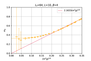
Repeating this extrapolation at different spatial sizes $L$ leads to good agreement with the conjectured proportionality relation $m_{\pi}^{\rm R}\propto 1/L$ , as Figure 3 shows for three $\beta$ -values.

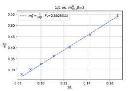
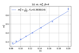
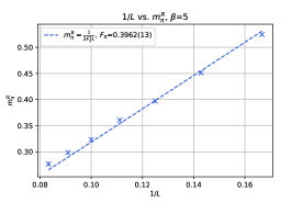
This allows us to employ eq. (16) and extract the value of $F_{\pi}$ — as defined in the $\delta$ -regime. The results at $\beta=3$ , $4$ and $5$ are given in Table 1.

$\beta$	$F_{\pi}$
3	0.3925(11)
4	0.3930(14)
5	0.3962(13)

Table 1:

F_{\pi}

obtained from

m_{\pi}^{\rm R}

in the

\delta

-regime, for three different

\beta

-values.

They agree very well for various values of $\beta$ . In addition, they are very close to the result for $F_{\pi}$ of Ref. [8], and to the results that we obtained based on the 2d Gell-Mann–Oakes–Renner relation, and on the Witten–Veneziano formula (if we assume $F_{\pi}=F_{\eta}$ ).

4 The chiral condensate

If we rely on the result (9), we can re-write the Gell-Mann–Oakes–Renner relation in the form

\Sigma=\frac{m_{\pi}^{2}}{4\pi m},

(17)

and use it to extract a value for the chiral condensate $\Sigma$ from the numerical solution of eqs. (2).

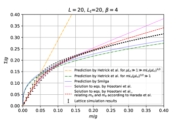
Figure 4 compares results for $\Sigma$ by a variety of approaches: the line linear in $m/g$ is the tangent at $m/g=0$ , which was correctly predicted in Ref. [11]. For our parameters, the corresponding conditions mean $8\gg 1$ (which is plausible), and $m/g\ll 0.035$ . However, the data follow well this straight line even up to $m/g\approx 0.035$ .

We add another small-mass predictions given in Ref. [11], which refers to the regime $m/g\gg 0.035$ , hence it should be valid in most of this plot, but it does not agree well with the lattice data (which are obtained with overlap fermions).

Next we show the line for a similar prediction from Ref. [7], which is not in accurate agreement with the lattice results either.

The solution of eqs. (2), inserted in relation (17), works better. It can be further improved if we replace the (somewhat troublesome) ansatz $m_{\eta}^{2}=m_{\pi}^{2}+\mu^{2}$ by a formula for $m_{\eta}$ , which is derived in Ref. [8].

Unlike Figs. 1 to 3, here we obtain an almost continuous line of lattice results, because we are using a single set of quenched configurations which are re-weighted by the fermion determinant to compute the chiral condensate for different fermion masses. As the ratio $m/g$ grows, we see that none of the theoretical predictions is truly successful, as we already observed in the case of the “meson” masses. We should add, however, that all these formulae refer to the continuum and an infinite spatial size, so the discrepancies could be (in part) due to finite-size effects and lattice artifacts.

5 Summary and mysteries

We presented lattice simulation results for the “meson” masses and the chiral condensate in the 2-flavor Schwinger model, and confronted them with a multitude of theoretical predictions. While some of them work well at small fermion mass $m$ , none of them is truly successful at moderate $m$ .

We also formulated the pion decay constant $F_{\pi}$ in various ways, by referring to different analogies to QCD. For three formulations we obtained consistent values, which are compatible with $F_{\pi}(m=0)=1/\sqrt{2\pi}$ , and with a previous study in Ref. [8]. This is very satisfactory, but there remain two open questions: 1. Why does the method based on the Witten–Veneziano formula require the identification $F_{\pi}=F_{\eta}\,$ ? 2. How can this be reconciled with relation (4), which suggests $F_{\pi}(m=0)=0\,$ ?

Acknowledgments: We thank the organizers of the XXXV Reunión Anual de la División de Partículas y Campos of the Sociedad Mexicana de Física, where this talk was presented by JFNC. We further thank Stephan Dürr and Christian Hoelbling for useful communication. The code development and testing were performed at the cluster Isabella of the Zagreb University Computing Centre (SRCE). The production runs were carried out on the cluster of the Instituto de Ciencias Nucleares, UNAM. This work was supported by UNAM-DGAPA through PAPIIT project IG100219, “Exploración teórica y experimental del diagrama de fase de la cromodinámica cuántica”, by the Consejo Nacional de Ciencia y Tecnología (CONACYT), and by the Faculty of Geotechnical Engineering (University of Zagreb, Croatia) through the project “Change of the Eigenvalue Distribution at the Temperature Transition” (2186-73-13-19-11).

\medline

References

$1$ .
$2$ . J. Schwinger, Gauge Invariance and Mass. 2., Phys. Rev. 128 (1962) 2425, 10.1103/PhysRev.128.2425.
$3$ . L. V. Belvedere, K. D. Rothe, B. Schroer and J. Swieca, Generalized Two-dimensional Abelian Gauge Theories and Confinement, Nucl. Phys. B 153 (1979) 112, 10.1016/0550-3213(79)90594-7.
$4$ . I. Hip, J. F. Nieto Castellanos and W. Bietenholz, Finite temperature and $\delta$ -regime in the 2-flavor Schwinger model, arXiv:2109.13468 [hep-lat].
$5$ . Y. Hosotani, More about the massive multiflavor Schwinger model, in Nihon University Workshop on Fundamental Problems in Particle Physics (1995) 64, [hep-th/9505168]. Y. Hosotani and R. Rodriguez, Bosonized massive N-flavor Schwinger model, J. Phys. A 31 (1998) 9925, 10.1088/0305-4470/31/49/013.
$6$ . J. F. Nieto Castellanos, The 2-flavor Schwinger model at finite temperature and in the delta-regime, B.Sc. thesis, Universidad Nacional Autónoma de México, 2021.
$7$ . A. V. Smilga, Critical amplitudes in two-dimensional theories, Phys. Rev. D 55 (1997) 443, 10.1103/PhysRevD.55.R443
$8$ . K. Harada, T. Sugihara, M. Taniguchi and M. Yahiro, The massive Schwinger model with $\textrm{SU(2)}_{f}$ on the light cone, Phys. Rev. D 49 (1994) 4226, 10.1103/PhysRevD.49.4226
$9$ . A. Smilga and J. J. M. Verbaarschot, Scalar susceptibility in QCD and the multiflavor Schwinger model, Phys. Rev. D 54 (1996) 1087, 10.1103/PhysRevD.54.1087
$10$ . A.V. Smilga, On the fermion condensate in the Schwinger model, Phys. Lett. B 278 (1992) 371, 10.1016/0370-2693(92)90209-M.
$11$ . J. Hetrick, Y. Hosotani and S. Iso, The massive multi-flavor Schwinger model, Phys. Lett. B 350 (1995) 92, 10.1016/0370-2693(95)00310-H
$12$ . E. Witten, Current Algebra Theorems for the U(1) Goldstone Boson, Nucl. Phys. B 156 (1979) 269, 10.1016/0550-3213(79)90031-2.
G. Veneziano, U(1) Without Instatons, Nucl. Phys. B 159 (1979) 213, 10.1016/0550-3213(79)90332-8
$13$ . C. Gattringer and E. Seiler, Functional integral approach to the N flavor Schwinger model, Annals Phys. 233 (1994) 97. 10.1006/aphy.1994.1062
$14$ . E. Seiler and I. O. Stamatescu, Some remarks on the Witten-Veneziano formula for the $\eta^{\prime}$ mass, Preprint MPI-PAE/PTh 10/87 (1987).
$15$ . W. A. Bardeen, A. Duncan, E. Eichten and H. Thacker, Quenched approximation artifacts: A study in two-dimensional QED, Phys. Rev. D 57 (1998) 3890, 10.1103/PhysRevD.57.3890.
S. Dürr and C. Hoelbling, Staggered versus overlap fermions: A Study in the Schwinger model with $N_{f}=0,\,1,\,2$ , Phys. Rev. D 69 (2004) 034503, 10.1103/PhysRevD.69.034503
C. Bonati and P. Rossi, Topological susceptibility of two-dimensional $U(N)$ gauge theories, Phys. Rev. D 99 (2019) 054503, 10.1103/PhysRevD.99.054503
$16$ . H. Leutwyler, Energy Levels of Light Quarks Confined to a Box, Phys. Lett. B 189 (1987) 197, 10.1016/0370-2693(87)91296-2
$17$ . P. Hasenfratz and F. Niedermayer, Finite size and temperature effects in the AF Heisenberg model, Z. Phys. B 92 (1993) 91, 10.1007/BF01309171