Neutrinophilic DM annihilation in a model
with $U(1)_{L_{\mu}-L_{\tau}}\times U(1)_{H}$ gauge symmetry

In the proposed scenario, we require all the scalar fields develop their vacuum expectation values (VEVs) to break electroweak and $U(1)_{L_{\mu}-L_{\tau}}\times U(1)_{H}$ gauge symmetries denoted by $\langle H\rangle\equiv[0,v/\sqrt{2}]^{T}$ and $\varphi_{1,2}\equiv v_{1,2}/\sqrt{2}$. Then, the scalar fields are written by

$$H=\left[\begin{array}[]{c}w^{+}\\ \frac{v+\tilde{h}+iz}{\sqrt{2}}\end{array}\right],\quad\varphi_{1,2}=\frac{v_{1,2}+\phi_{1,2}+iz^{\prime}_{1,2}}{\sqrt{2}},$$

(5)

where $w^{+}$ and $z$ are massless Nambu-Goldstone(NG) bosons which are absorbed by the SM gauge bosons $W^{+}$ and $Z$, and linear combinations of $z^{\prime}_{1,2}$ become NG bosons absorbed by two extra neutral gauge bosons from $U(1)_{L_{\mu}-L_{\tau}}\times U(1)_{H}$. The VEVs are obtained by conditions $\frac{\partial{\cal V}}{\partial v}=\frac{\partial{\cal V}}{\partial v_{1}}=\frac{\partial{\cal V}}{\partial v_{2}}=0$ that are written by

	$\displaystyle v\left(\mu_{H}^{2}+\frac{\lambda_{H\varphi_{1}}}{2}v_{1}^{2}+\frac{\lambda_{H\varphi_{2}}}{2}v_{2}^{2}\right)+\lambda_{H}v^{3}=0,$		(6)
	$\displaystyle v_{1}\left(\mu_{1}^{2}+\frac{\lambda_{H\varphi_{1}}}{2}v^{2}+\frac{\lambda_{\varphi_{1}\varphi_{2}}}{2}v_{2}^{2}\right)+\lambda_{1}v_{1}^{3}=0,$		(7)
	$\displaystyle v_{2}\left(\mu_{2}^{2}+\frac{\lambda_{H\varphi_{2}}}{2}v^{2}+\frac{\lambda_{\varphi_{1}\varphi_{2}}}{2}v_{1}^{2}\right)+\lambda_{2}v_{2}^{3}=0.$		(8)

After the scalar fields developing VEVs, neutral scalars $\tilde{h}$, $\phi_{1}$ and $\phi_{2}$ mix. We assume the mixings between $\tilde{h}$ and $\phi_{1,2}$ are small for simplicity and $\tilde{h}$ is identified as the SM Higgs boson. Other scalar bosons are not involved in our phenomenological analysis below and we do not discuss further details in this work ²²2Collider signatures from a scalar boson decaying into $Z^{\prime}$ in the context of $U(1)_{L_{\mu}-L_{\tau}}$ are discussed in refs. Das:2022mmh ; Nomura:2020vnk ; Nomura:2018yej . .

After spontaneous symmetry breaking, we obtain mass terms for the gauge fields such that

$\displaystyle|D_{\mu}\varphi_{1}|^{2}+|D_{\mu}\varphi_{2}|^{2}\supset\frac{1}{2}g^{2}_{\mu\tau}(v_{1}^{2}+v_{2}^{2})X^{\mu}_{1}X_{1\mu}+\frac{1}{2}g^{2}_{H}v^{2}_{2}X^{\mu}_{2}X_{2\mu}+g_{\mu\tau}g_{H}v_{2}^{2}X^{\mu}_{1}X_{2\mu}.$

(9)

We thus obtain mass matrix in the basis of $\{X^{\mu}_{1},X^{\mu}_{2}\}$ as

$$M_{X_{1}X_{2}}^{2}=\begin{pmatrix}M^{2}_{1}&M^{2}_{12}\\ M^{2}_{12}&M^{2}_{2}\end{pmatrix},$$

(10)

where $M^{2}_{1}\equiv g^{2}_{\mu\tau}(v_{1}^{2}+v_{2}^{2})$, $M^{2}_{2}\equiv g^{2}_{H}v^{2}_{2}$ and $M^{2}_{12}\equiv g_{H}g_{\mu\tau}v^{2}_{2}$. We can diagonalize the mass matrix by orthogonal matrix, and mass eigenvalues and eigenstates are written by

	$\displaystyle m^{2}_{Z^{\prime}_{1}}=\frac{1}{2}(M^{2}_{1}+M^{2}_{2})+\frac{1}{2}\sqrt{(M^{2}_{1}-M^{2}_{2})^{2}+4M^{4}_{12}}\ ,$		(11)
	$\displaystyle m^{2}_{Z^{\prime}_{2}}=\frac{1}{2}(M^{2}_{1}+M^{2}_{2})-\frac{1}{2}\sqrt{(M^{2}_{1}-M^{2}_{2})^{2}+4M^{4}_{12}}\ ,$		(12)
	$\displaystyle\begin{pmatrix}X_{1}^{\mu}\\ X^{\mu}_{2}\end{pmatrix}=\begin{pmatrix}\cos\theta_{X}&\sin\theta_{X}\\ -\sin\theta_{X}&\cos\theta_{X}\end{pmatrix}\begin{pmatrix}Z^{\prime\mu}_{1}\\ Z^{\prime\mu}_{2}\end{pmatrix},$		(13)

where the mixing angle $\theta_{X}$ is obtained from

$$\tan 2\theta_{X}=\frac{2M^{2}_{12}}{M^{2}_{1}-M^{2}_{2}}.$$

(14)

In our scenario, we consider the case of $m_{Z^{\prime}_{1}}\gg m_{Z^{\prime}_{2}}$ by choosing gauge couplings and VEVs accordingly. Then $Z^{\prime}_{1}$ interaction is applied to explain $B$ decay anomalies while $Z^{\prime}_{2}$ dominantly contributes to induce sizable muon $g-2$.

In mass basis, we write relevant new gauge interactions as

	$\displaystyle\mathcal{L}\supset\$	$\displaystyle g_{\mu\tau}(c_{X}Z^{\prime\mu}_{1}+s_{X}Z^{\prime\mu}_{2})(\bar{\mu}\gamma_{\mu}\mu-\bar{\tau}\gamma_{\mu}\tau)+g_{\mu\tau}(c_{X}Z^{\prime\mu}_{1}+s_{X}Z^{\prime\mu}_{2})(\overline{\nu_{\mu}}\gamma_{\mu}P_{L}\nu_{\mu}-\overline{\nu_{\tau}}\gamma_{\mu}P_{L}\nu_{\tau})$
		$\displaystyle+Q_{\chi}g_{H}(-s_{X}Z^{\prime\mu}_{1}+c_{X}Z^{\prime\mu}_{2})\bar{\chi}\gamma_{\mu}\chi,$		(15)

where $c_{X}(s_{X})=\cos\theta_{X}(\sin\theta_{X})$.

Our $Z^{\prime}$ bosons can decay into leptons $\{\mu\bar{\mu},\tau\bar{\tau},\nu_{\mu}\bar{\nu}_{\mu},\nu_{\tau}\bar{\nu}_{\tau}\}$ and $\chi\bar{\chi}$ when these modes are kinematically allowed. Partial decay widths of the $Z^{\prime}_{1}$ and $Z^{\prime}_{2}$ bosons are given by

	$\displaystyle\Gamma(Z^{\prime}_{1}\to\ell^{\prime}\bar{\ell}^{\prime})$	$\displaystyle=\frac{c_{X}^{2}g^{2}_{\mu\tau}}{8\pi}m_{Z^{\prime}_{1}}\left(1+\frac{4}{3}\frac{m_{\ell^{\prime}}^{2}}{m^{2}_{Z^{\prime}_{1}}}\sqrt{1-\frac{4m^{2}_{\ell^{\prime}}}{m^{2}_{Z^{\prime}_{1}}}}\right),$
	$\displaystyle\Gamma(Z^{\prime}_{1}\to\nu_{\ell^{\prime}}\bar{\nu}_{\ell^{\prime}})$	$\displaystyle=\frac{c_{X}^{2}g^{2}_{\mu\tau}}{8\pi}m_{Z^{\prime}_{1}},$
	$\displaystyle\Gamma(Z^{\prime}_{1}\to\chi\bar{\chi})$	$\displaystyle=\frac{Q_{\chi}^{2}s_{X}^{2}g^{2}_{H}}{8\pi}m_{Z^{\prime}_{1}}\left(1+\frac{4}{3}\frac{m_{\chi}^{2}}{m^{2}_{Z^{\prime}_{1}}}\sqrt{1-\frac{4m^{2}_{\chi}}{m^{2}_{Z^{\prime}_{1}}}}\right),$
	$\displaystyle\Gamma(Z^{\prime}_{2}\to\ell^{\prime}\bar{\ell}^{\prime})$	$\displaystyle=\frac{s_{X}^{2}g^{2}_{\mu\tau}}{8\pi}m_{Z^{\prime}_{2}}\left(1+\frac{4}{3}\frac{m_{\ell^{\prime}}^{2}}{m^{2}_{Z^{\prime}_{2}}}\sqrt{1-\frac{4m^{2}_{\ell^{\prime}}}{m^{2}_{Z^{\prime}_{2}}}}\right),$
	$\displaystyle\Gamma(Z^{\prime}_{2}\to\nu_{\ell^{\prime}}\bar{\nu}_{\ell^{\prime}})$	$\displaystyle=\frac{s_{X}^{2}g^{2}_{\mu\tau}}{8\pi}m_{Z^{\prime}_{2}},$
	$\displaystyle\Gamma(Z^{\prime}_{2}\to\chi\bar{\chi})$	$\displaystyle=\frac{Q_{\chi}^{2}c_{X}^{2}g^{2}_{H}}{8\pi}m_{Z^{\prime}_{2}}\left(1+\frac{4}{3}\frac{m_{\chi}^{2}}{m^{2}_{Z^{\prime}_{2}}}\sqrt{1-\frac{4m^{2}_{\chi}}{m^{2}_{Z^{\prime}_{2}}}}\right),$		(16)

where $\ell^{\prime}=\{\mu,\tau\}$. When the $Z^{\prime}_{1,2}$ boson mass is $\mathcal{O}(10)$ GeV to $\mathcal{O}(100)$ GeV, their couplings and masses are strongly constrained by LHC data searching for $pp\to\mu^{+}\mu^{-}Z^{\prime}(\to\mu^{+}\mu^{-})$ signal CMS:2018yxg . We can also find other constraints in the context of $L_{\mu}-L_{\tau}$ scenario in ref. Chun:2018ibr which are subdominant in the scenario of this work. The constraint can be relaxed when $Z^{\prime}_{1,2}$ dominantly decays into $\chi\bar{\chi}$. We will take this constraint into account in our numerical analysis below.

In our model, both the $Z^{\prime}_{1}$ and $Z^{\prime}_{2}$ bosons contribute to muon $g-2$ since they interact with muon as given by Eq. (II.3). Calculating one-loop diagrams, we obtain muon $g-2$ such that

$$\Delta a_{\mu}=\frac{g^{2}_{\mu\tau}m^{2}_{\mu}}{4\pi}\int_{0}^{1}dx\left[c_{X}^{2}\frac{x^{2}(1-x)}{x^{2}+(1-x)r_{Z^{\prime}_{1}}}+s_{X}^{2}\frac{x^{2}(1-x)}{x^{2}+(1-x)r_{Z^{\prime}_{2}}}\right],$$

(17)

where $r_{Z^{\prime}_{1(2)}}\equiv m_{Z^{\prime}_{1(2)}}^{2}/m^{2}_{\mu}$. We apply the $3\sigma$ region obtained by combining FNAL and BNL results that require new contribution to satisfy

$$(25.1-3\times 5.9)\times 10^{-10}\leq\Delta a^{\rm new}_{\mu}\leq(25.1+3\times 5.9)\times 10^{-10}.$$

(18)

This constraint is imposed in our numerical calculation below.

Neutrino trident production processes, $\nu+N\to\nu+N+\mu+\bar{\mu}$, are neutrino scattering off nucleus producing a muon and anti-muon pair. The cross section of the muon neutrino trident has been measured by past experiments, CHARM-II CHARM-II:1990dvf , CCFR CCFR:1991lpl and NuTeV NuTeV:1999wlw . The current limits on the total cross section are respectively given by

	$\displaystyle\frac{\sigma_{\mathrm{CHARM-II}}}{\sigma_{\mathrm{SM}}}$	$\displaystyle=1.58\pm 0.57,$		(19)
	$\displaystyle\frac{\sigma_{\mathrm{CCFR}}}{\sigma_{\mathrm{SM}}}$	$\displaystyle=0.82\pm 0.28,$		(20)
	$\displaystyle\frac{\sigma_{\mathrm{NuTeV}}}{\sigma_{\mathrm{SM}}}$	$\displaystyle=0.72^{+1.73}_{-0.72},$		(21)

where $\sigma_{\mathrm{SM}}$ is the SM prediction Belusevic:1987cw ³³3The cross sections were calculated in the V-A theory in Refs.Czyz:1964zz ; Lovseth:1971vv ; Fujikawa:1973vu ; Koike:1971tu ; Koike:1971vg ; Brown:1972vne ..

It was shown in Altmannshofer:2014pba that these limits severely constrain the $Z^{\prime}$ mass and its coupling to neutrinos. The sensitivity in on-going and future experiments have been studied, e.g. in Kaneta:2016uyt ; Araki:2017wyg ; Magill:2016hgc ; Ge:2017poy ; Falkowski:2018dmy ; Altmannshofer:2019zhy ; Shimomura:2020tmg . The trident cross section of this model can be obtained by simply replacing the coupling of the SM as

$\displaystyle g_{L/R}\to g_{L/R}-\frac{\sqrt{2}g_{\mu\tau}^{2}}{4G_{F}}\sum_{i}\frac{a_{i}}{q^{2}-m^{2}_{Z_{i}^{\prime}}},$

(22)

where $a_{1}=c_{X}^{2},~{}a_{2}=s_{X}^{2}$ and $g_{L/R}$ is

	$\displaystyle g_{L}$	$\displaystyle=\frac{1}{2}+\sin^{2}\theta_{W},$		(23)
	$\displaystyle g_{R}$	$\displaystyle=\sin^{2}\theta_{W}.$		(24)

The concrete forms of the amplitudes are given in Shimomura:2020tmg .

To obtain the constraints from the tridents, we have calculated the cross section for CHARM-II and CCFR and compared them with the SM predictions⁴⁴4The result from NuTeV has large uncertainty and includes the null result. Therefore we do not use this result..

Firstly we review the mechanisms to explain B decay anomalies by $Z^{\prime}$ boson from local $U(1)_{L_{\mu}-L_{\tau}}$. The anomalies can be explained if we have a quark flavor violating interaction $Z^{\prime}_{\mu}\bar{b}\gamma^{\mu}P_{L}s$ and $Z^{\prime}$-muon interaction $Z^{\prime}_{\nu}\bar{\mu}\gamma^{\nu}\mu$. These interactions induce an effective interaction

$$\mathcal{H}_{\rm eff}=-\frac{4G_{F}}{\sqrt{2}}V_{tb}V^{*}_{ts}\frac{\alpha}{4\pi}C_{9}(\bar{b}\gamma^{\nu}P_{L}s)(\bar{\mu}\gamma_{\nu}\mu),$$

(25)

where the $C_{9}$ is a corresponding Wilson coefficient, $G_{F}$ is the Fermi constant, $V_{tb}$ and $V_{ts}$ are elements of CKM matrix, and $\alpha$ is the fine structure constant. To induce $Z^{\prime}_{\mu}\bar{b}\gamma^{\mu}P_{L}s$, we need new fields since the $Z^{\prime}$ boson from $U(1)_{L_{\mu}-L_{\tau}}$ does not interact with quarks. Possible ways to induce such a flavor violating interaction can be achieved as follows.

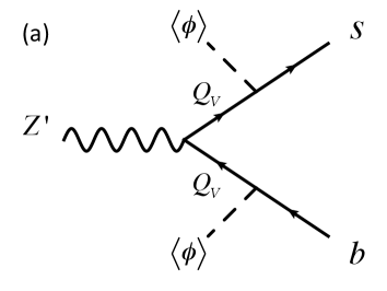
1. 1.

   $Z^{\prime}_{\mu}\bar{b}\gamma^{\mu}P_{L}s$ interaction is induced via mixing between $U(1)_{L_{\mu}-L_{\tau}}$ charged vector-like quark $Q_{V}$ and the SM ones Altmannshofer:2014cfa . We also need a new scalar field $\phi$ with $U(1)_{L_{\mu}-L_{\tau}}$ charge to connect a vector-like quark and SM ones after developing its VEV. An example of diagram inducing the interaction by mixing effect is shown in Fig. 1(a).

2. 2.

   The interaction is induced at one-loop level by introducing a vector-like quark $Q_{V}$ and new scalar field $\eta$ that are charged under $U(1)_{L_{\mu}-L_{\tau}}$ Ko:2017yrd ; Chen:2017usq . An example of diagram inducing the interaction by radiative correction is shown in Fig. 1(b). Interestingly, a scalar field $\eta$ can be DM candidate.

In fact, they can be obtained by the same field contents, a vector-like quark $Q_{V}$ and a scalar field ($\phi=\eta$) charged under a new $U(1)$ gauge group(s), where the difference is whether new scalar develops a VEV or not. In this paper, we do not discuss details and we just assume effective $X_{1(2)\mu}\bar{b}\gamma^{\mu}P_{L}s$ couplings induced by one of such mechanisms.

In our analysis, we just write effectively induced interactions by

$$\mathcal{L}_{\rm eff}=(g^{L}_{bsX_{1}}X^{\mu}_{1}+g^{L}_{bsX_{2}}X^{\mu}_{2})\overline{b_{L}}\gamma_{\mu}s_{L},$$

(26)

where we consider couplings $g^{L}_{bsX_{1,2}}$ are free parameters. In mass basis of the gauge bosons $\{Z^{\prime\mu}_{1},Z^{\prime\mu}_{2}\}$, the interaction is rewritten by

	$\displaystyle\mathcal{L}_{\rm eff}$	$\displaystyle=\left[(g^{L}_{bsX_{1}}c_{X}-g^{L}_{bsX_{2}}s_{X})Z^{\prime\mu}_{1}+(g^{L}_{bsX_{1}}s_{X}+g^{L}_{bsX_{2}}c_{X})Z^{\prime\mu}_{2}\right]\overline{b_{L}}\gamma_{\mu}s_{L}$
		$\displaystyle\equiv\left[g^{L}_{bsZ^{\prime}_{1}}Z^{\prime\mu}_{1}+g^{L}_{bsZ^{\prime}_{2}}Z^{\prime\mu}_{2}\right]\overline{b_{L}}\gamma_{\mu}s_{L}.$		(27)

Hereafter we consider $g^{L}_{bsZ^{\prime}_{1}}$ and $g^{L}_{bsZ^{\prime}_{2}}$ as free parameters.

From $Z^{\prime}$ exchanging diagram, we obtain contribution to the Wilson coefficient $C_{9}$ that is required to explain $B$ anomalies. Here we assume $g^{L}_{bsZ^{\prime}_{1}}\gg g^{L}_{bsZ^{\prime}_{2}}$ that is required by constraints from $B\to K^{(*)}Z^{\prime}$ decay as can be seen in the next subsection. Then contribution to $C_{9}$ from $Z^{\prime}_{1}$ exchange is given by

$$C_{9}^{Z^{\prime}}\simeq-\frac{\pi c_{X}g_{\mu\tau}g^{L}_{bsZ^{\prime}_{1}}}{\sqrt{2}V_{tb}V^{*}_{ts}\alpha G_{F}m_{Z^{\prime}_{1}}^{2}}.$$

(28)

Constraint from $B_{s}$–$\overline{B_{s}}$ mixing : the effective interactions in Eq. (26) also induce the mixing between $B_{s}$ and $\overline{B_{s}}$ mesons, and a constraint from the meson mixing should be considered. We can find the ratio of $B_{s}$–$\overline{B_{s}}$ mixing between SM and $Z^{\prime}$ contributions as Tuckler:2022fkz ; Altmannshofer:2016jzy

$$\frac{M^{Z^{\prime}}_{12}}{M^{\rm SM}_{12}}\simeq\frac{(g^{L}_{bsZ^{\prime}_{1}})^{2}}{m_{Z^{\prime}_{1}}^{2}}\frac{16\sqrt{2}\pi^{2}}{g^{2}G_{F}(V_{tb}V^{*}_{ts})^{2}S_{0}},$$

(29)

where $S_{0}\simeq 2.3$ is the SM loop function Inami:1980fz ; Buchalla:1995vs . Note that we ignored a contribution from $Z^{\prime}_{2}$ since we adopt assumption of $g^{L}_{bsZ^{\prime}_{1}}\gg g^{L}_{bsZ^{\prime}_{2}}$. Then we rewrite $g^{L}_{bsZ^{\prime}_{1}}$ in terms of $C_{9}^{Z^{\prime}}$ from Eq. (28) as follows:

$$g^{L}_{bsZ^{\prime}_{1}}=\sqrt{2}V_{tb}V^{*}_{ts}\frac{\alpha}{\pi}G_{F}C_{9}^{Z^{\prime}}\frac{m_{Z^{\prime}_{1}}^{2}}{c_{X}g_{\mu\tau}}.$$

(30)

Requiring $|M^{Z^{\prime}}_{12}|/|M^{{\rm SM}}_{12}|<0.12$ Charles:2020dfl , we obtain the constraint

$$m_{Z^{\prime}_{1}}<2.1\ {\rm TeV}\times\frac{c_{X}g_{\mu\tau}}{|C_{9}^{Z^{\prime}}|}.$$

(31)

We apply the constraint assuming $C_{9}^{Z^{\prime}}=-1.01$ that is the best-fit value in our numerical analysis below.

In our scenario we consider light $Z^{\prime}_{2}$ to explain muon $g-2$, and we should take into account constraints from $B\to K^{(*)}Z^{\prime}$ decay processes that are induced by quark flavor violating coupling in Eq. (II.6). We can estimate decay widths such that Crivellin:2022obd

	$\displaystyle\Gamma(B\to KZ^{\prime}_{2})=\frac{(g^{L}_{sbZ^{\prime}_{2}})^{2}f^{2}_{+}(m_{Z^{\prime}_{2}}^{2})}{16\pi m_{B}^{2}m^{2}_{Z^{\prime}_{2}}}\lambda(m_{B}^{2},m_{K}^{2},m_{Z^{\prime}_{2}}^{2})^{\frac{3}{2}},$		(32)
	$\displaystyle\Gamma(B\to K^{*}Z^{\prime}_{2})$
	$\displaystyle=\frac{(g^{L}_{sbZ^{\prime}_{2}})^{2}V^{2}(m^{2}_{Z^{\prime}})}{8\pi m_{B}^{2}(m_{B}+m_{K^{*}})^{2}}\lambda(m_{B}^{2},m_{K^{*}}^{2},m_{Z^{\prime}}^{2})^{\frac{3}{2}}+\frac{(g^{L}_{sbZ^{\prime}_{2}})^{2}A_{2}^{2}(m^{2}_{Z^{\prime}_{2}})}{64\pi m_{B}^{2}m_{K^{*}}^{2}m^{2}_{Z^{\prime}}(m_{B}+m_{K^{*}})^{2}}\lambda(m_{B}^{2},m_{K^{*}}^{2},m_{Z^{\prime}_{2}}^{2})^{\frac{5}{2}}$
	$\displaystyle+\frac{(g^{L}_{sbZ^{\prime}_{2}})^{2}A_{1}^{2}(m^{2}_{Z^{\prime}_{2}})[m_{B}^{4}+m^{4}_{K^{*}}+m^{4}_{Z^{\prime}}+10m^{2}_{Z^{\prime}_{2}}m^{2}_{K^{*}}-2m^{2}_{B}(m^{2}_{K^{*}}+m^{2}_{Z^{\prime}_{2}})]}{64\pi m_{B}^{2}m_{K^{*}}^{2}m_{Z^{\prime}_{2}}^{2}}\lambda(m_{B}^{2},m_{K^{*}}^{2},m_{Z^{\prime}_{2}}^{2})^{\frac{1}{2}}$
	$\displaystyle+\frac{(g^{L}_{sbZ^{\prime}_{2}})^{2}A_{1}(m^{2}_{Z^{\prime}_{2}})A_{2}(m^{2}_{Z^{\prime}_{2}})(m_{B}^{2}-m^{2}_{K^{*}}-m^{2}_{Z^{\prime}_{2}})}{32\pi m_{B}^{2}m_{K^{*}}^{2}m^{2}_{Z^{\prime}_{2}}}\lambda(m_{B}^{2},m_{K^{*}}^{2},m_{Z^{\prime}_{2}}^{2})^{\frac{3}{2}},$		(33)

where $\lambda(x,y,z)=x^{2}+y^{2}+z^{2}-2xy-2xz-2yz$ and $\{f_{+},V,A_{1},A_{2}\}$ are form factors for $B$ and $K^{(*)}$ mesons Bailey:2015dka . In our scenario, we require $m_{Z^{\prime}_{2}}<2m_{\mu}$ and $Z^{\prime}_{2}$ decays into neutrinos or DM that are not observed by the detectors at the experiments searching for rare $B$ decay modes. We note that narrow width approximation is relevant in our case for $Z^{\prime}_{2}$ decay. We consider $Z^{\prime}_{2}$ decaying into only neutrinos in considering the constraint and decay width is narrow since corresponding coupling is $g_{\mu\tau}\sin\theta_{X}\lesssim 0.5\times 0.1$ in our scenario. We then adopt the following experimental constraints Belle:2017oht ; Belle-II:2021rof

	$\displaystyle BR(B\to K\nu\bar{\nu})<1.6\times 10^{-5},\qquad BR(B\to K^{*}\nu\bar{\nu})<2.7\times 10^{-5},$
	$\displaystyle BR(B^{+}\to K^{+}\nu\bar{\nu})<4.1\times 10^{-5}.$		(34)

We find that constraint becomes stronger when we take $q^{2}$ dependence of detector efficiency into account for $B^{+}\to K^{+}\nu\bar{\nu}$ search Belle-II:2021rof since the efficiency is higher for small $q^{2}$ region ($q^{2}=m_{Z^{\prime}_{2}}^{2}\lesssim(0.2\ {\rm GeV})^{2}$). But we find that the strongest upper bounds of effective coupling $g^{L}_{bsZ^{\prime}_{2}}$ for our benchmark points are obtained from constraint on $BR(B\to K^{*}\nu\bar{\nu})$ when we assume efficiency for $B\to K^{*}Z^{\prime}(\to\nu\bar{\nu})$ is the same as that of $B\to K^{*}\bar{\nu}\nu$ in the SM since $q^{2}$ dependence other than $B^{+}\to K^{+}\nu\bar{\nu}$ is not known ⁵⁵5The constraint could be stronger when we take $q^{2}$ dependence into account since efficiency at small $q^{2}$ region could be higher as in the $B^{+}\to K^{+}\nu\bar{\nu}$ search..

In our analysis, relevant free parameters are

$$\{g_{\mu\tau},g_{H},v_{1},v_{2}\},$$

(35)

and our outputs are $\{m_{Z^{\prime}_{1}},m_{Z^{\prime}_{2}},\sin\theta_{X},\Delta a_{\mu}\}$ obtained from formulae in the previous section. The charge $Q_{X}$ for DM is chosen to be $1$ for simplicity. We scan our free parameters in the following range:

$\displaystyle g_{\mu\tau}\in[10^{-3},10^{-1}],\quad g_{H}\in[10^{-3},0.5],\quad v_{1}\in[10^{2},10^{4}]\ {\rm GeV},\quad v_{2}\in[1,10^{3}]\ {\rm GeV}.$

(36)

We then require the following conditions in addition to Eq. (18);

$\displaystyle m_{Z^{\prime}_{1}}>5\ {\rm GeV},\quad m_{Z^{\prime}_{2}}<0.2\ {\rm GeV},$

(37)

where the first constraint is motivated to explain $b\to s\ell^{+}\ell^{-}$ anomalies and the second constraint is imposed to realize DM annihilation into neutrinos. In addition, we require $Z^{\prime}_{1}$ dominantly decaying into $\chi\bar{\chi}$ by making $\Gamma(Z^{\prime}_{1}\to\chi\bar{\chi})\gg\Gamma(Z^{\prime}_{1}\to\ell^{\prime}\bar{\ell}^{\prime},\nu_{\ell}\bar{\nu}_{\ell^{\prime}})$ in Eq. (II.3) imposing the condition

$$\frac{g_{\mu\tau}\cos\theta_{X}}{g_{H}\sin\theta_{X}}<3,$$

(38)

in order to relax the constraint from the LHC search for $pp\to\mu^{+}\mu^{-}Z^{\prime}(\to\mu^{+}\mu^{-})$ signal.

In Fig. 2, we show the ratio of neutrino trident cross section between the SM one and the one including contributions from both the SM and $Z^{\prime}$ bosons $\sigma_{Z^{\prime}}$. The plots in the left(right) sides express the ratio as functions of $Z^{\prime}_{1(2)}$ mass. The upper(lower) plots correspond to the ratio in CCFR(CHARM-II) experiments. The shaded region is excluded by the experiments by 90 $\%$ confidence level (CL). We find some parameter points are excluded where lighter $Z^{\prime}_{1}$ region and/or heavier $Z^{\prime}_{2}$ region tend to be constrained inducing a larger ratio.

In the left panel of Fig. 3, we show correlation between $v_{1}$ and $v_{2}$ for our allowed parameter region. In addition, the right panel of Fig. 3 shows the correlation between two new gauge couplings. We find some correlation between them when we require masses of $Z^{\prime}_{1,2}$ as Eq. (37) and muon $g-2$ within $3\sigma$ CL.

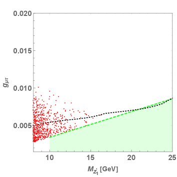
In left(right) plots of Fig. 4, we show the allowed parameter region that satisfies the constraints from neutrino trident and induces sizable muon $g-2$ within 3$\sigma$ CL, on $\{m_{Z^{\prime}_{1}},g_{\mu\tau}\}$ ($\{m_{Z^{\prime}_{2}},g_{\mu\tau}\sin\theta_{X}\}$) plane. The green shaded region in the left plot is disfavored when we explain $b\to s\ell^{+}\ell^{-}$ anomalies via $Z^{\prime}_{1}$ interaction. Also, for comparison, we added a dotted curve in the same plot indicating the LHC constraint from $pp\to\mu^{+}\mu^{-}Z^{\prime}(\to\mu^{+}\mu^{-})$ signal search when $Z^{\prime}_{1}$ does not decay into DM; this is not relevant in our case since $Z^{\prime}_{1}$ dominantly decays into DM under our requirement in Eq. (38). We also show excluded region from “$e^{+}e^{-}\to\mu^{+}\mu^{-}+\text{invisible}$” search at the Belle II experiment Belle-II:2019qfb as blue shaded region in the right panel of Fig. 4 ⁶⁶6There is another constraint from “$pp\to\mu^{+}\mu^{-}+\text{anything}$” search Bishara:2017pje when $Z^{\prime}_{1,2}$ mass is few GeV scale. We omit the excluded region since the mass region is outside the plots in Fig. 4. Note also that more parameter region can be tested searching for the “$e^{+}e^{-}\to\mu^{+}\mu^{-}+\text{invisible}$” process at the future LHC experiments Elahi:2015vzh ; analysis in the reference indicates that coupling region of $g_{\mu\tau}\sin\theta_{X}\gtrsim 3\times 10^{-4}$ can be tested for $m_{Z^{\prime}_{2}}<2m_{\mu}$ at the HL-LHC with 3 ab^-1 integrated luminosity.

In order to discuss DM physics, we choose several benchmark points from our allowed parameter region. In Table 2, we summarize benchmark points (BPs) that satisfy $\Delta a_{\mu}$ within $1\sigma$ C.L. where we also show effective coupling $g_{bsZ^{\prime}_{1}}$ giving $C_{9}^{Z^{\prime}}=-1.01$ and the upper limit of $g_{bsZ^{\prime}_{2}}$ avoiding $B$ meson decay constraints.

References

- (1) B. Abi et al. [Muon g-2], Phys. Rev. Lett. 126 (2021) no.14, 141801 doi:10.1103/PhysRevLett.126.141801 [arXiv:2104.03281 [hep-ex]].
- (2) K. Hagiwara, R. Liao, A. D. Martin, D. Nomura and T. Teubner, J. Phys. G 38, 085003 (2011) [arXiv:1105.3149 [hep-ph]].
- (3) T. Aoyama, M. Hayakawa, T. Kinoshita and M. Nio, Phys. Rev. Lett. 109, 111808 (2012) doi:10.1103/PhysRevLett.109.111808 [arXiv:1205.5370 [hep-ph]].
- (4) T. Aoyama, T. Kinoshita and M. Nio, Atoms 7, no.1, 28 (2019) doi:10.3390/atoms7010028
- (5) A. Czarnecki, W. J. Marciano and A. Vainshtein, Phys. Rev. D 67, 073006 (2003) [erratum: Phys. Rev. D 73, 119901 (2006)] doi:10.1103/PhysRevD.67.073006 [arXiv:hep-ph/0212229 [hep-ph]].
- (6) C. Gnendiger, D. Stöckinger and H. Stöckinger-Kim, Phys. Rev. D 88, 053005 (2013) doi:10.1103/PhysRevD.88.053005 [arXiv:1306.5546 [hep-ph]].
- (7) A. Keshavarzi, D. Nomura and T. Teubner, Phys. Rev. D 97, no.11, 114025 (2018) doi:10.1103/PhysRevD.97.114025 [arXiv:1802.02995 [hep-ph]].
- (8) G. Colangelo, M. Hoferichter and P. Stoffer, JHEP 02, 006 (2019) doi:10.1007/JHEP02(2019)006 [arXiv:1810.00007 [hep-ph]].
- (9) M. Hoferichter, B. L. Hoid and B. Kubis, JHEP 08, 137 (2019) doi:10.1007/JHEP08(2019)137 [arXiv:1907.01556 [hep-ph]].
- (10) A. Keshavarzi, D. Nomura and T. Teubner, Phys. Rev. D 101, no.1, 014029 (2020) doi:10.1103/PhysRevD.101.014029 [arXiv:1911.00367 [hep-ph]].
- (11) A. Kurz, T. Liu, P. Marquard and M. Steinhauser, Phys. Lett. B 734, 144-147 (2014) doi:10.1016/j.physletb.2014.05.043 [arXiv:1403.6400 [hep-ph]].
- (12) K. Melnikov and A. Vainshtein, Phys. Rev. D 70, 113006 (2004) doi:10.1103/PhysRevD.70.113006 [arXiv:hep-ph/0312226 [hep-ph]].
- (13) P. Masjuan and P. Sanchez-Puertas, Phys. Rev. D 95, no.5, 054026 (2017) doi:10.1103/PhysRevD.95.054026 [arXiv:1701.05829 [hep-ph]].
- (14) G. Colangelo, M. Hoferichter, M. Procura and P. Stoffer, JHEP 04, 161 (2017) doi:10.1007/JHEP04(2017)161 [arXiv:1702.07347 [hep-ph]].
- (15) M. Hoferichter, B. L. Hoid, B. Kubis, S. Leupold and S. P. Schneider, JHEP 10, 141 (2018) doi:10.1007/JHEP10(2018)141 [arXiv:1808.04823 [hep-ph]].
- (16) A. Gérardin, H. B. Meyer and A. Nyffeler, Phys. Rev. D 100, no.3, 034520 (2019) doi:10.1103/PhysRevD.100.034520 [arXiv:1903.09471 [hep-lat]].
- (17) J. Bijnens, N. Hermansson-Truedsson and A. Rodríguez-Sánchez, Phys. Lett. B 798, 134994 (2019) doi:10.1016/j.physletb.2019.134994 [arXiv:1908.03331 [hep-ph]].
- (18) G. Colangelo, F. Hagelstein, M. Hoferichter, L. Laub and P. Stoffer, JHEP 03, 101 (2020) doi:10.1007/JHEP03(2020)101 [arXiv:1910.13432 [hep-ph]].
- (19) T. Blum, N. Christ, M. Hayakawa, T. Izubuchi, L. Jin, C. Jung and C. Lehner, Phys. Rev. Lett. 124, no.13, 132002 (2020) doi:10.1103/PhysRevLett.124.132002 [arXiv:1911.08123 [hep-lat]].
- (20) G. Colangelo, M. Hoferichter, A. Nyffeler, M. Passera and P. Stoffer, Phys. Lett. B 735, 90-91 (2014) doi:10.1016/j.physletb.2014.06.012 [arXiv:1403.7512 [hep-ph]].
- (21) M. Davier, A. Hoecker, B. Malaescu and Z. Zhang, Eur. Phys. J. C 77, no.12, 827 (2017) doi:10.1140/epjc/s10052-017-5161-6 [arXiv:1706.09436 [hep-ph]].
- (22) M. Davier, A. Hoecker, B. Malaescu and Z. Zhang, Eur. Phys. J. C 80, no.3, 241 (2020) [erratum: Eur. Phys. J. C 80, no.5, 410 (2020)] doi:10.1140/epjc/s10052-020-7792-2 [arXiv:1908.00921 [hep-ph]].
- (23) S. Borsanyi, Z. Fodor, J. N. Guenther, C. Hoelbling, S. D. Katz, L. Lellouch, T. Lippert, K. Miura, L. Parato and K. K. Szabo, et al. Nature 593 (2021) no.7857, 51-55 doi:10.1038/s41586-021-03418-1 [arXiv:2002.12347 [hep-lat]].
- (24) C. Alexandrou, S. Bacchio, P. Dimopoulos, J. Finkenrath, R. Frezzotti, G. Gagliardi, M. Garofalo, K. Hadjiyiannakou, B. Kostrzewa and K. Jansen, et al. [arXiv:2206.15084 [hep-lat]].
- (25) M. Cè, A. Gérardin, G. von Hippel, R. J. Hudspith, S. Kuberski, H. B. Meyer, K. Miura, D. Mohler, K. Ottnad and P. Srijit, et al. [arXiv:2206.06582 [hep-lat]].
- (26) A. Crivellin, M. Hoferichter, C. A. Manzari and M. Montull, arXiv:2003.04886 [hep-ph].
- (27) E. de Rafael, Phys. Rev. D 102 (2020) no.5, 056025 [arXiv:2006.13880 [hep-ph]].
- (28) A. Keshavarzi, W. J. Marciano, M. Passera and A. Sirlin, Phys. Rev. D 102 (2020) no.3, 033002 doi:10.1103/PhysRevD.102.033002 [arXiv:2006.12666 [hep-ph]].
- (29) M. Passera, W. J. Marciano and A. Sirlin, Phys. Rev. D 78 (2008), 013009 [arXiv:0804.1142 [hep-ph]].
- (30) W. Altmannshofer, S. Gori, S. Profumo and F. S. Queiroz, JHEP 12 (2016), 106 [arXiv:1609.04026 [hep-ph]].
- (31) D. Tuckler, [arXiv:2209.03397 [hep-ph]].
- (32) P. Ko, T. Nomura and H. Okada, Phys. Rev. D 95 (2017) no.11, 111701 [arXiv:1702.02699 [hep-ph]].
- (33) C. H. Chen and T. Nomura, Phys. Lett. B 777 (2018), 420-427 [arXiv:1707.03249 [hep-ph]].
- (34) A. Crivellin, G. D’Ambrosio and J. Heeck, Phys. Rev. Lett. 114, 151801 (2015) [arXiv:1501.00993 [hep-ph]].
- (35) A. Crivellin, G. D’Ambrosio and J. Heeck, Phys. Rev. D 91, no.7, 075006 (2015) [arXiv:1503.03477 [hep-ph]].
- (36) S. Baek, JHEP 05, 104 (2019) [arXiv:1901.04761 [hep-ph]].
- (37) Z. L. Han, R. Ding, S. J. Lin and B. Zhu, Eur. Phys. J. C 79, no.12, 1007 (2019) [arXiv:1908.07192 [hep-ph]].
- (38) N. Kumar, T. Nomura and H. Okada, Chin. Phys. C 46 (2022) no.4, 043106 [arXiv:2002.12218 [hep-ph]].
- (39) W. Chao, H. Wang, L. Wang and Y. Zhang, Chin. Phys. C 45, no.8, 083105 (2021) [arXiv:2102.07518 [hep-ph]].
- (40) D. Borah, M. Dutta, S. Mahapatra and N. Sahu, [arXiv:2109.02699 [hep-ph]].
- (41) W. Altmannshofer, S. Gori, M. Pospelov and I. Yavin, Phys. Rev. D 89 (2014), 095033 [arXiv:1403.1269 [hep-ph]].
- (42) A. Crivellin, C. A. Manzari, W. Altmannshofer, G. Inguglia, P. Feichtinger and J. Martin Camalich, Phys. Rev. D 106 (2022) no.3, L031703 doi:10.1103/PhysRevD.106.L031703 [arXiv:2202.12900 [hep-ph]].
- (43) G. Hiller and F. Kruger, Phys. Rev. D 69, 074020 (2004) [hep-ph/0310219].
- (44) C. Bobeth, G. Hiller and G. Piranishvili, JHEP 0712, 040 (2007) [arXiv:0709.4174 [hep-ph]].
- (45) R. Aaij et al. [LHCb Collaboration], Phys. Rev. Lett. 113, 151601 (2014) [arXiv:1406.6482 [hep-ex]].
- (46) R. Aaij et al. [LHCb], Phys. Rev. Lett. 122 (2019) no.19, 191801 [arXiv:1903.09252 [hep-ex]].
- (47) R. Aaij et al. [LHCb], [arXiv:2103.11769 [hep-ex]].
- (48) S. Descotes-Genon, J. Matias, M. Ramon and J. Virto, JHEP 1301, 048 (2013) [arXiv:1207.2753 [hep-ph]].
- (49) R. Aaij et al. [LHCb Collaboration], JHEP 1602, 104 (2016) [arXiv:1512.04442 [hep-ex]].
- (50) R. Aaij et al. [LHCb Collaboration], Phys. Rev. Lett. 111, 191801 (2013) [arXiv:1308.1707 [hep-ex]].
- (51) A. Abdesselam et al. [Belle Collaboration], arXiv:1604.04042 [hep-ex].
- (52) S. Wehle et al. [Belle Collaboration], arXiv:1612.05014 [hep-ex].
- (53) R. Aaij et al. [LHCb], JHEP 08 (2017), 055 [arXiv:1705.05802 [hep-ex]].
- (54) [LHCb], [arXiv:2212.09152 [hep-ex]].
- (55) [LHCb], [arXiv:2212.09153 [hep-ex]].
- (56) A. Das, T. Nomura and T. Shimomura, [arXiv:2212.11674 [hep-ph]].
- (57) T. Nomura and T. Shimomura, Eur. Phys. J. C 81 (2021) no.4, 297 [arXiv:2012.13049 [hep-ph]].
- (58) T. Nomura and T. Shimomura, Eur. Phys. J. C 79 (2019) no.7, 594 [arXiv:1803.00842 [hep-ph]].
- (59) T. Inami and C. S. Lim, Prog. Theor. Phys. 65 (1981), 297 [erratum: Prog. Theor. Phys. 65 (1981), 1772] doi:10.1143/PTP.65.297
- (60) G. Buchalla, A. J. Buras and M. E. Lautenbacher, Rev. Mod. Phys. 68 (1996), 1125-1144 doi:10.1103/RevModPhys.68.1125 [arXiv:hep-ph/9512380 [hep-ph]].
- (61) J. Charles, S. Descotes-Genon, Z. Ligeti, S. Monteil, M. Papucci, K. Trabelsi and L. Vale Silva, Phys. Rev. D 102 (2020) no.5, 056023 doi:10.1103/PhysRevD.102.056023 [arXiv:2006.04824 [hep-ph]].
- (62) A. M. Sirunyan et al. [CMS], Phys. Lett. B 792 (2019), 345-368 doi:10.1016/j.physletb.2019.01.072 [arXiv:1808.03684 [hep-ex]].
- (63) E. J. Chun, A. Das, J. Kim and J. Kim, JHEP 02, 093 (2019) [erratum: JHEP 07, 024 (2019)] doi:10.1007/JHEP02(2019)093 [arXiv:1811.04320 [hep-ph]].
- (64) J. A. Bailey, A. Bazavov, C. Bernard, C. M. Bouchard, C. DeTar, D. Du, A. X. El-Khadra, J. Foley, E. D. Freeland and E. Gámiz, et al. Phys. Rev. D 93 (2016) no.2, 025026 doi:10.1103/PhysRevD.93.025026 [arXiv:1509.06235 [hep-lat]].
- (65) J. Grygier et al. [Belle], Phys. Rev. D 96 (2017) no.9, 091101 doi:10.1103/PhysRevD.96.091101 [arXiv:1702.03224 [hep-ex]].
- (66) G. Belanger, F. Boudjema, A. Pukhov and A. Semenov, Comput.¥ Phys.¥ Commun.¥ ¥bf 192, 322 (2015) [arXiv:1407.6129 [hep-ph]].
- (67) N. Aghanim et al. [Planck], Astron. Astrophys. 641, A6 (2020) [erratum: Astron. Astrophys. 652, C4 (2021)] doi:10.1051/0004-6361/201833910 [arXiv:1807.06209 [astro-ph.CO]].
- (68) S. Palomares-Ruiz and S. Pascoli, Phys. Rev. D 77, 025025 (2008) doi:10.1103/PhysRevD.77.025025 [arXiv:0710.5420 [astro-ph]].
- (69) A. Olivares-Del Campo, C. Bœhm, S. Palomares-Ruiz and S. Pascoli, Phys. Rev. D 97, no.7, 075039 (2018) doi:10.1103/PhysRevD.97.075039 [arXiv:1711.05283 [hep-ph]].
- (70) C. A. Argüelles, A. Diaz, A. Kheirandish, A. Olivares-Del-Campo, I. Safa and A. C. Vincent, Rev. Mod. Phys. 93, no.3, 035007 (2021) doi:10.1103/RevModPhys.93.035007 [arXiv:1912.09486 [hep-ph]].
- (71) N. F. Bell, M. J. Dolan and S. Robles, JCAP 09, 019 (2020) doi:10.1088/1475-7516/2020/09/019 [arXiv:2005.01950 [hep-ph]].
- (72) K. Akita, G. Lambiase, M. Niibo and M. Yamaguchi, JCAP 10, 097 (2022) doi:10.1088/1475-7516/2022/10/097 [arXiv:2206.06755 [hep-ph]].
- (73) J. F. Navarro, C. S. Frenk and S. D. M. White, Astrophys. J. 462, 563-575 (1996) doi:10.1086/177173 [arXiv:astro-ph/9508025 [astro-ph]].
- (74) M. Benito, A. Cuoco and F. Iocco, JCAP 03, 033 (2019) doi:10.1088/1475-7516/2019/03/033 [arXiv:1901.02460 [astro-ph.GA]].
- (75) B. Moore, T. R. Quinn, F. Governato, J. Stadel and G. Lake, Mon. Not. Roy. Astron. Soc. 310, 1147-1152 (1999) doi:10.1046/j.1365-8711.1999.03039.x [arXiv:astro-ph/9903164 [astro-ph]].
- (76) J. N. Bahcall and R. M. Soneira, , ApJS 44 (1980) 73
- (77) D. Geiregat et al. [CHARM-II], Phys. Lett. B 245, 271-275 (1990) doi:10.1016/0370-2693(90)90146-W
- (78) S. R. Mishra et al. [CCFR], Phys. Rev. Lett. 66, 3117-3120 (1991) doi:10.1103/PhysRevLett.66.3117
- (79) T. Adams et al. [NuTeV], Phys. Rev. D 61, 092001 (2000) doi:10.1103/PhysRevD.61.092001 [arXiv:hep-ex/9909041 [hep-ex]].
- (80) R. Belusevic and J. Smith, Phys. Rev. D 37, 2419 (1988) doi:10.1103/PhysRevD.37.2419
- (81) W. Czyz, G. C. Sheppey and J. D. Walecka, Nuovo Cim. 34, 404-435 (1964) doi:10.1007/BF02734586
- (82) J. Lovseth and M. Radomiski, Phys. Rev. D 3, 2686-2706 (1971) doi:10.1103/PhysRevD.3.2686
- (83) K. Fujikawa, Annals Phys. 75, 491-502 (1973) doi:10.1016/0003-4916(73)90078-X
- (84) K. Koike, M. Konuma, K. Kurata and K. Sugano, Prog. Theor. Phys. 46, 1150-1169 (1971) doi:10.1143/PTP.46.1150
- (85) K. Koike, M. Konuma, K. Kurata and K. Sugano, Prog. Theor. Phys. 46, 1799-1804 (1971) doi:10.1143/PTP.46.1799
- (86) R. W. Brown, R. H. Hobbs, J. Smith and N. Stanko, Phys. Rev. D 6, 3273-3292 (1972) doi:10.1103/PhysRevD.6.3273
- (87) W. Altmannshofer, S. Gori, M. Pospelov and I. Yavin, Phys. Rev. Lett. 113, 091801 (2014) doi:10.1103/PhysRevLett.113.091801 [arXiv:1406.2332 [hep-ph]].
- (88) Y. Kaneta and T. Shimomura, PTEP 2017, no.5, 053B04 (2017) doi:10.1093/ptep/ptx050 [arXiv:1701.00156 [hep-ph]].
- (89) T. Araki, S. Hoshino, T. Ota, J. Sato and T. Shimomura, Phys. Rev. D 95, no.5, 055006 (2017) doi:10.1103/PhysRevD.95.055006 [arXiv:1702.01497 [hep-ph]].
- (90) G. Magill and R. Plestid, Phys. Rev. D 95, no.7, 073004 (2017) doi:10.1103/PhysRevD.95.073004 [arXiv:1612.05642 [hep-ph]].
- (91) S. F. Ge, M. Lindner and W. Rodejohann, Phys. Lett. B 772, 164-168 (2017) doi:10.1016/j.physletb.2017.06.020 [arXiv:1702.02617 [hep-ph]].
- (92) A. Falkowski, G. Grilli di Cortona and Z. Tabrizi, JHEP 04, 101 (2018) doi:10.1007/JHEP04(2018)101 [arXiv:1802.08296 [hep-ph]].
- (93) W. Altmannshofer, S. Gori, J. Martín-Albo, A. Sousa and M. Wallbank, Phys. Rev. D 100, no.11, 115029 (2019) doi:10.1103/PhysRevD.100.115029 [arXiv:1902.06765 [hep-ph]].
- (94) T. Shimomura and Y. Uesaka, Phys. Rev. D 103, no.3, 035022 (2021) doi:10.1103/PhysRevD.103.035022 [arXiv:2009.13773 [hep-ph]].
- (95) F. Abudinén et al. [Belle-II], Phys. Rev. Lett. 127 (2021) no.18, 181802 doi:10.1103/PhysRevLett.127.181802 [arXiv:2104.12624 [hep-ex]].
- (96) I. Adachi et al. [Belle-II], Phys. Rev. Lett. 124 (2020) no.14, 141801 doi:10.1103/PhysRevLett.124.141801 [arXiv:1912.11276 [hep-ex]].
- (97) F. Bishara, U. Haisch and P. F. Monni, Phys. Rev. D 96 (2017) no.5, 055002 doi:10.1103/PhysRevD.96.055002 [arXiv:1705.03465 [hep-ph]].
- (98) F. Elahi and A. Martin, Phys. Rev. D 93 (2016) no.1, 015022 doi:10.1103/PhysRevD.93.015022 [arXiv:1511.04107 [hep-ph]].
- (99) K. Asai, K. Hamaguchi, N. Nagata, S. Y. Tseng and K. Tsumura, Phys. Rev. D 99 (2019) no.5, 055029 doi:10.1103/PhysRevD.99.055029 [arXiv:1811.07571 [hep-ph]].
- (100) K. Asai, K. Hamaguchi and N. Nagata, Eur. Phys. J. C 77 (2017) no.11, 763 doi:10.1140/epjc/s10052-017-5348-x [arXiv:1705.00419 [hep-ph]].