[figure]captionskip=0pt,font=footnotesize \floatsetup[subfigure]captionskip=0pt,font=footnotesize
Neutrino Lorentz invariance violation from the even SME coefficients through a tensor interaction with cosmological scalar fields
Abstract
Numerous non-standard interactions between neutrinos and scalar fields have been suggested in the literature. In this work, we have outlined the case of tensorial neutrino non-standard interactions with scalar fields, which can be related to the effective even dimension4 operators of the Standard Model Extension (SME). We illustrate how bounds placed on these parameters can be associated with limits on the energy scale of the proposed neutrino interactions with cosmic scalars. Besides, as a case study, we employ a DUNE-like experimental configuration to assess the projected sensitivities to the even isotropic and spatial SME coefficients. For the case of the isotropic SME coefficients, an upper limit on the energy scale of the interaction can be placed. The current IceCube experiment and upcoming neutrino experiments such as DUNE, KM3NeT, IceCube-Gen2, and GRAND proposals, may clarify these classes of neutrino non-standard interactions.
I Introduction
The discovery of the Universe’s accelerating expansion Riess et al. (1998); Perlmutter et al. (1999) is one of the most important, captivating, and puzzling open questions in cosmology Sahni (2004); Alam et al. (2004). Several proposals to architecture Dark Matter (DM) and Dark Energy (DE) have been investigated in the literature. The Lambda Cold Dark Matter (CDM) model is among the most popular explanations for cosmological observations, although recent results from the Dark Energy Spectroscopic Instrument (DESI) Adame et al. (2024) show some tension with this model. Different candidates for DM particles have been considered, ranging in a very wide mass spectrum, making the Weakly Interacting Massive Particle (WIMP) paradigm one of the best motivated from a theoretical point of view Arbey and Mahmoudi (2021). However, despite thorough searches for WIMPs, they all have failed to find any signature.
Other DM and DE candidates have also been studied in an effort to find a plausible explanation to the cosmological observations. For instance, ultralight scalars are well-motivated proposals for cosmological DM Magana and Matos (2012); Ferreira (2021); Suárez et al. (2014); Hui et al. (2017); Matos et al. (2024). Moreover, several ultralight scalars become apparent within the context of string theories Arvanitaki et al. (2010); Cicoli et al. (2022); Acharya et al. (2010); Marsh (2016). 111Some strategies to hunt for ultralight scalars as cosmological DM involve atomic clocks Arvanitaki et al. (2015), resonant-mass detectors Arvanitaki et al. (2016) and atomic gravitational wave detectors Arvanitaki et al. (2018). Scalar fields minimally coupled to gravity are sufficiently justified models of DE Li et al. (2011), namely quintessence Wetterich (1988); Zlatev et al. (1999), symmetrons Kading:2023hdb ; Burrage:2018zuj , and k-essence Chiba et al. (2000); Armendariz-Picon et al. (2000, 2001); Melchiorri et al. (2003); Chiba (2002); Chimento and Feinstein (2004); Chimento (2004).
In k-essence models, the scalar field plays a significant role in describing the DE puzzle. This field could have adequate behavior at early epochs and can reproduce the dynamical effects of the cosmological constant at late times. Classes of k-essence Lagrangians were introduced in several settings, for example, as a possible model for inflation Armendariz-Picon et al. (1999); Garriga and Mukhanov (1999). Subsequently, k-essence models were used as another possibility to describe the characteristics of DE and as an alternative mechanism for unifying DE and DM Scherrer (2004). Purely kinetic k-essence models de Putter and Linder (2007); Gao and Yang (2010) are, in a way, as simple as quintessence models, because they rely only on one function () through the expression of the Lagrangian density , where is the kinetic term.
Among other proposals, there are second-order derivative scalar field models, or generalized galileons Nicolis et al. (2009); de Rham and Tolley (2010); Goon et al. (2011a, b), with the property that their equations of motion are second-order.
Interesting examples of this class of models are the so-called kinetic gravity braiding models, that are formulated from a Lagrangian that includes a D’Alambertian operator and an arbitrary function of a non-canonical kinetic term giving rise to appealing cosmological effects Deffayet et al. (2010); Pujolas et al. (2011); Kimura and Yamamoto (2011); Maity (2013).
At the cosmological level, all the aforementioned models of DM and DE can be described as a perfect fluid through their energy-momentum tensor Weinberg (2008). At present, discrimination among them could be done at the level of the energy-momentum tensor perturbations. On the other hand, the search for signatures confirming the existence of scalars is an important challenge. Proposals considering the interaction of scalar fields with neutrinos have demonstrated that a possible signature might be detected in long-baseline neutrino experiments Berlin (2016); de Salas et al. (2016); Krnjaic et al. (2018); Brdar et al. (2018); Smirnov and Xu (2019); Dev et al. (2021); Losada et al. (2022, 2023); Huang et al. (2022); Cordero et al. (2023); Sen and Smirnov (2024) or via modifications to the ultrahigh energy neutrino fluxes Barranco et al. (2011); Reynoso and Sampayo (2016). Besides, it has also been argued that interactions of neutrinos with scalars, if they exist, could induce an apparent violation of Lorentz and symmetries in the neutrino sector Gu et al. (2007); Ando et al. (2009); Klop and Ando (2018); Capozzi et al. (2018); Farzan and Palomares-Ruiz (2019); Ge and Murayama (2019); Gherghetta and Shkerin (2023); Argüelles et al. (2023a, b); Lambiase and Poddar (2024); Cordero and Delgadillo (2024); Argüelles et al. (2024). These scalars can be identified as either DM or DE candidates. We refer to Kostelecky and Mewes (2004a); Diaz (2016); Torri (2020); Moura and Rossi-Torres (2022); Barenboim (2022) for comprehensive reviews concerning Lorentz and symmetry violations in the neutrino sector, within the Standard Model Extension (SME) framework Colladay and Kostelecky (1998). An initial proposal for violation in the neutrino sector was discussed in Ref. Barenboim and Lykken (2003).
Recently, there has been an increased interest in searches for Lorentz invariance and breakdowns in neutrino oscillation experiments Barenboim et al. (2019); Abbasi et al. (2022); Sahoo et al. (2022); Agarwalla et al. (2023); Raikwal et al. (2023); Crivellin:2020oov ; Testagrossa et al. (2023); Shukla:2024fnw . For instance, comprehensive studies of the isotropic even SME coefficient, , at different long-baseline experiments can be found in Refs. Agarwalla et al. (2023); Raikwal et al. (2023). 222As shown in Díaz et al. (2020), it is possible to relate the isotropic SME coefficients with the effects of the violation of the equivalence principle (VEP) in the neutrino sector. Besides, there is a correspondence between quantum-decoherence effects in neutrinos and the effective coefficients of the SME Barenboim and Mavromatos (2005); De Romeri et al. (2023); Barenboim and Gago (2024). In Ref. Delgadillo:2024bae , we examine the phenomenology of isotropic and anisotropic odd SME coefficients, and , considering the Deep Underground Neutrino Experiment (DUNE) Abi et al. (2020a) configuration.
In this paper, we consider the possibility of tensorial neutrino non-standard interactions with scalar fields; such as quintessence and other related DE models, as well as the case of ultralight dark matter (ULDM). We focus on the scenario where the even SME coefficients could correspond to a tensorial interaction of neutrinos with cosmological scalar fields. In this scenario, an apparent Lorentzviolating signature may manifest and give a sizable signal at upcoming and present neutrino oscillation experiments. Besides, as a case of study, we asses the projected sensitivities of a DUNE-like setup to these types of LIV scenarios. This is the first time sensitivities for the even SME coefficients at DUNE are presented.
The manuscript is organized as follows: In Section II, we introduce the theoretical foundations, where the basics of Lorentz invariance violations are presented together with the necessary Lagrangian formalism to describe the several models of scalar fields useful to model DM and DE. In Section III, we describe the phenomenology of a tensorial neutrino interaction with scalar fields as either DM or DE candidates and its connection with the even SME coefficients . In Section IV, we assess the sensitivities to the even SME coefficients, , considering the DUNE configuration. Finally, we give our conclusions.
II Theoretical framework
Within the SME framework, violations of Lorentz invariance (LIV) in the fermion sector, are parameterized by the effective Lagrangian Barenboim (2022)
| (1) |
where is the Standard Model (SM) fermion Lagrangian, being the Lorentz and violating Lagrangian term,
| (2) |
In the case of neutrinos, it is convenient to define
| (3) |
where the coefficients are odd, while the coefficients are even. These type of conserving terms, , were studied in the context of a Finslerian Geometrical model Antonelli et al. (2018), violations of diffeomorphism invariance Reyes:2024hqi ; Santos:2024iyc , and neutrino interactions with a k-essence field Gauthier et al. (2010). For other scenarios of neutrinodark energy interactions, we refer the reader to Refs. Khalifeh and Jimenez (2021a, b, 2022).
Lately, it has been suggested that violations of Lorentz invariance and symmetry in the neutrino sector may arise from a neutrinocurrent coupled with a dynamical cosmic field, (see, e.g., Refs. Gu et al. (2007); Ando et al. (2009); Klop and Ando (2018); Capozzi et al. (2018); Argüelles et al. (2023b); Lambiase and Poddar (2024); Cordero and Delgadillo (2024))
| (4) |
being some coupling constants, the energy scale of the interaction, and a timevarying scalar field, which could be identified as either a dark matter or dark energy candidate. 333For ultra-relativistic neutrinos, the phenomenology with axion-like dark matter is the same as the ultralight dark matter scenario Lambiase and Poddar (2024); Gherghetta and Shkerin (2023); Huang and Nath (2018). Here, violations of the Lorentz and symmetries emerge via the odd SME coefficients .
Motivated by the aforementioned proposals, let us consider the corresponding free scalar field Lagrangian and its energy-momentum tensor, which are relevant for describing both, scalar field dark matter and dark energy quintessence Weinberg (2008); Ferreira (2021); Wetterich (1988),
| (5) |
Therefore, the scalar field energy-momentum tensor can be expressed as
| (6) |
and we identify the density and pressure of the scalar field as
| (7) |
The scalar field four-velocity, , is given as
| (8) |
The isotropy and homogeneity of space-time require the stress-energy-momentum tensor for a free scalar field, , to be that of a perfect fluid,
| (9) |
subject to the constraint . The conservation of in a Friedmann-Lemaitre-Robertson-Walker (FLRW) background leads to the continuity equation,
| (10) |
which gives the equation of motion of the scalar field,
| (11) |
Nevertheless, dark energy can be modeled by a k-essence field which has very appealing properties and is described by the Lagrangian density Armendariz-Picon et al. (2000) which is associated with the following energy-momentum tensor,
| (12) |
where is the kinetic term and . The energy density and pressure are given by
| (13) |
respectively, and the equation of motion can be obtained from the continuity equation,
| (14) |
where and .
Another possible interesting scalar field used to describe the dark energy evolution is the braided scalar field described by the Lagrangian:
| (15) |
where and the function is arbitrary Pujolas et al. (2011). The energy-momentum tensor, , in covariant form, is given by
| (16) |
where , and . This energy-momentum tensor can be described in terms of an imperfect fluid Pujolas et al. (2011) . We start defining some quantities to describe relativistic fluids. A local rest frame is set defining the normalized four-velocity
| (17) | |||
| (18) |
with is the four-acceleration which is orthogonal to velocity, . The expansion, , and the diffusivity, , are written as
| (19) |
where . The energy-momentum tensor also can be expressed in this way:
| (20) |
where is the chemical potential, is the heat flux (purely spatial, ) and is the transverse projector. The energy density and isotropic pressure are:
| (21) | |||||
| (22) |
The conservation of using these definitions can be expressed as:
| (23) |
The equation of motion for can be obtained from the last equation
| (24) |
In the cosmological background, the evolution of the scalar field reduces to the dynamics of a perfect fluid which is described only through its energy density and pressure.
III Tensorial neutrino LIV
Consider the effective Lagrangian (see Appendix A for further details)
| (25) |
being a coupling constant matrix, the energy scale of the interaction, and is the tensor associated to the scalar field , for instance those of Eqs. (6), (12), and (16). Hence, we can identify the even LIV coefficients of the SME as
| (26) |
Here, the scalar field could be one of the DM or DE candidates described in Section II. Besides, the effective interaction (Eq. 25) may induce potential scattering among the neutrinos and the scalar particles. However, such interactions would be expected to be negligible (see Appendix B of Ref. Klop and Ando (2018)). Henceforth, we discuss the case of a tensorial neutrino-scalar field interaction. 444A study of the the back-reaction effects from the tensorial neutrino-scalar field interaction is beyond the scope of this work.
III.1 Isotropic LIV coefficients from a neutrino-scalar field interaction
From the effective Lagrangian in Eq. (25), the corresponding isotropic -even LIV coefficients are
| (27) |
considering the scalar field as ultralight dark matter (ULDM) Suárez et al. (2014); Ferreira (2021), with corresponding local DM density in the Milky Way, eV4 de Salas et al. (2019); de Salas and Widmark (2021); Sivertsson et al. (2022), an accelerator-based experiment similar to DUNE, with sensitivity (left panel of Fig. 1 in Sec. IV), could potentially probe an energy scale of the interaction
| (28) |
On the other hand, if the scalar field is considered to be a DE candidate, namely quintessence, the corresponding dark energy density eV4, in this scenario, the DUNE setup could potentially probe an energy scale
| (29) |
At the cosmological level, the aforementioned models of dark energy outlined in Section II, can be described by a dynamical scalar field , thus, for all cases, they would predict . However, limits from astrophysical neutrinos ( PeV) employing the IceCube astrophysical neutrino flavour data-set constraint Abbasi et al. (2022) (such limits are expected to be improved by the combination of a two-detector fit, namely IceCube-Gen2 and GRAND Testagrossa et al. (2023)), therefore 555Besides, in the standard model, neutrinos are part of the doublet, hence, we could have potentially induced LIV effects for the charged leptons. However, for the case of electrons, limits from astrophysical observations constraint Kostelecky and Russell (2011), which are several orders of magnitude weaker than the constraints derived in the neutrino sector Abbasi et al. (2022).
| (30) |
considering as DM, ultra-high energy (UHE) neutrino experiments could potentially be sensitive to an energy scale
| (31) |
on the other hand, considering as DE, UHE neutrino experiments could potentially be sensitive to an energy scale
| (32) |
In Table. 2, we display the energy scale reach at IceCube as well as other neutrino experiments. Besides, considering only the derivative coupling on the scalar fields (see Appendix A), unitarity bounds in collisions with quarks at the LHC set GeV, while unitarity bounds from LEP when colliding electrons and positrons impose GeV Brax and Burrage (2014).
III.2 Directional dependent LIV coefficients from a neutrino-scalar field interaction
Searches of directional dependent LIV effects can be performed at neutrino experiments such as the KM3NeT neutrino telescope and the IceCube neutrino observatory, with neutrino energies GeV Klop and Ando (2018); Telalovic and Bustamante (2023). For instance, regarding directional dependent Lorentz violating effects in the direction, the projected sensitivities of a neutrino long-baseline experiment similar to DUNE to the even spatial LIV coefficients are, (right panel of Fig. 1 in Sec. IV) and (right panel of Fig. 2 in Sec. IV), both at 95% C.L., accordingly.
From the phenomenological Lagrangian in Eq. (25), the corresponding even spatial LIV coefficients in terms of the scalar field tensor are
| (33) |
where accounts for the perturbations of the scalar field tensor . However, perturbations for the several dark energy models outlined: quintessence, k-essence, or kinetic gravity braiding models, are expected to be different. 666A detail study of the energy-momentum perturbations for these models is beyond the scope of this paper and we leave it for a future work. Subsequently, we refer to the dark energy quintessence model for simplicity. Still, a similar phenomenology applies to the other dark energy models.
The perturbed stress-energy-momentum tensor for the scalar field , with perturbation in the FLRW background with a Newtonian gauge is given as Magana and Matos (2012)
| (34) |
Considering as ULDM, from the equation of state of the scalar field , with , the leading contribution , hence, in this case the even spatial LIV coefficients are
| (35) |
here plays the role of the gravitational potential, while is the scalar field perturbation Magana and Matos (2012). On the other hand, if is a DE candidate (quintessence) from the equation of state of the scalar field , with ,
| (36) |
For instance, in Table. 2, we show the energy scale reach within this scenario, considering limits set on the even SME coefficients () from several neutrino experimental configurations. In a similar fashion, considering as either ULDM or DE quintessence, the leading contribution (Eq. 9), therefore, the even coefficients from the sector can be described as
| (37) |
IV Numerical analysis and expected sensitivities
Long-baseline neutrino oscillation experiments play a significant role in both deciphering mysteries within the traditional three-neutrino oscillation picture and exploring other novel physics scenarios, including the potential breaking of the Lorentz and symmetries. Hence, as a case of study, we will focus on a long-baseline experimental configuration, the Deep Underground Neutrino Experiment (DUNE), which is a next-generation accelerator-based neutrino oscillation experiment that will consist of up to 40 kt of liquid argon (far) detector located at the Sanford underground research facility (SURF) in South Dakota Abi et al. (2020b). Moreover, this configuration is expected to deliver a neutrino flux with a mean neutrino energy 3 GeV, which will be located at a distance of 1300 km from the beam source (on-axis) at Fermilab (we refer the reader to Refs. Agarwalla et al. (2023); Abi et al. (2020a), for a detailed discussion regarding the experimental configuration).
In order to obtain sensitivities to the LIV coefficients at DUNE, we use the GLoBES software Huber et al. (2005, 2007) and its additional NSI tool snu.c Kopp (2008); Kopp et al. (2007) which was modified to implement the even coefficients of the SME at the Hamiltonian level. Moreover, to simulate the DUNE configuration, we employ the available GLoBES ancillary files Abi et al. (2021) and specifications from the Technical Design Report (TDR) configuration Abi et al. (2020a). Furthermore, in this work, we have contemplated a year running time, evenly distributed among neutrino and anti-neutrino modes. To simulate the DUNE event spectra, we consider the reconstructed neutrino and anti-neutrino energy range from 0 to 18 GeV for both appearance and disappearance channels. While elaborating our sensitivity plots, we performed a full spectral analysis with a total of 70 bins in the aforementioned energy range (having non-uniform bin widths). We have 64 bins each having a width of 0.125 GeV in the energy range of 0 to 8 GeV, and 6 bins with variable widths beyond 8 GeV Abi et al. (2021).
In this analysis, we have considered the following Hamiltonian
| (38) |
here, and are the standard neutrino Hamiltonian in vacuum and matter, respectively. Besides, is the contribution from the Lorentz invariance violation (LIV) sector, which can be parameterized as Kostelecky and Mewes (2004b); Diaz et al. (2009); Mishra et al. (2023)
| (39) |
where is the neutrino energy, are the even LIV coefficients of the SME (being , and ), for non-diagonal , (from now on, we will denote , and ), and
| (40) |
is the spatial component factor, expressed in terms of local spherical coordinates at the detector, that represents the direction of neutrino propagation in the Sun-centered frame. Being the colatitude of the detector, the angle at the detector between the beam direction and vertical, and the angle between the beam and east of south Kostelecky and Mewes (2004b). In the particular case of the DUNE location, Delgadillo:2024bae .
IV.1 Sensitivity to even SME coefficients
In order to assess the statistical significance to even SME coefficients, we employ a chi-squared test, we have considered the muon neutrino disappearance channel as well as the electron neutrino appearance channel , from a muon-neutrino beam with neutrino and antineutrino data sets. 777A detailed discussion of the impact of the even SME coefficients in the neutrino oscillation probability is beyond of the scope of this work. The total function is provided as in Ref. Cordero et al. (2023)
| (41) |
where the corresponding function for each channel (), appearance or disappearance is given as in Ref. Huber et al. (2002)
| (42) |
here, refers to the simulated events at the -th energy bin (considering the standard three neutrino oscillations picture), while are the computed events at the -th energy bin including even SME coefficients (one parameter at a time). In addition, is the set of neutrino oscillation parameters, while is the set of either isotropic (), spatial () or () SME coefficients, where are the nuisance parameters to account for the systematic uncertainties. Furthermore, are the systematic uncertainties as reported in the DUNE TDR Abi et al. (2020a). Besides, to obtain our simulated events; we have considered the corresponding neutrino oscillation parameters as true values, namely , , , , , and , corresponding to the best-fit values with normal mass ordering (NO) from Ref. de Salas et al. (2021) as displayed in Tab. 1.
| Oscillation parameter | best-fit NO |
|---|---|
| 34.3∘ | |
| 49.26∘ | |
| 8.53∘ | |
| [10-5 eV2] | 7.5 |
| [10-3 eV2] | 2.55 |
| 1.08 |
Furthermore, to include external input and marginalization for the standard oscillation parameters (in the total function), Gaussian priors Huber et al. (2002) are utilized,
| (43) |
the central values of the oscillation parameter priors () were fixed to their best-fit de Salas et al. (2021), considering the normal mass ordering, is the uncertainty on the oscillation prior, which corresponds to a 1 error (68.27% confidence level C.L. ).

In Fig. 1, we display our results of the expected 95% C.L. sensitivities to the non-diagonal SME coefficients, namely the isotropic (left panel) and spatial (right panel), for the DUNE configuration. Here, we have marginalized over the corresponding LIV phases and from [0], as well as the atmospheric mixing angle and the leptonic phase , considering a 1 uncertainty of 10% and 15% around their NO best-fit values, as displayed in Table 1. All the remaining oscillation parameters were fixed to their best fit value with normal mass ordering de Salas et al. (2021). Our results of the projected sensitivities to the isotropic LIV coefficients , are in agreement with those from Refs. Agarwalla et al. (2023); Raikwal et al. (2023). However, main differences arising on the total number of bins and energy range selected for the reconstructed neutrino energies, as well as the neutrino oscillation benchmark values considered in the calculation of the expected number of events.
To put our results in perspective, existing bounds from the Super-Kamiokande experiment constraint and at 95 C.L. Abe et al. (2015), while IceCube sets with a Bayes factor Abbasi et al. (2022). Furthermore, a test for Lorentz and violation with the MiniBooNE low-energy excess restrict Katori (2010); Kostelecky and Russell (2011), while limits from the Double Chooz experiment set Re Katori and Spitz (2014). For projected sensitivities and some experimental constraints on the LIV coefficients, and , see Tab. 2.
Regarding the diagonal SME coefficients and , we have fixed , as well as , since we can redefine the diagonal elements up to a global constant.


Our results of the projected 95% C.L. sensitivities to the (left panel) and (right panel) coefficients at the DUNE experiment are shown in Fig. 2. We have marginalized over the corresponding atmospheric mixing angle and Dirac -violating phase , considering a 1 uncertainty of 10% and 15% around their NO best-fit values, as show in Table 1. All the remaining oscillation parameters were fixed to their best fit value with normal mass ordering de Salas et al. (2021). We observe that the DUNE will be able to set limits on the isotropic -even SME coefficients and , while for the spatial LIV coefficients and , all of them at 95% confidence level. For instance, the null observation of LIV at the IceCube neutrino observatory constraint Re and Re with a Bayes factor Abbasi et al. (2022).


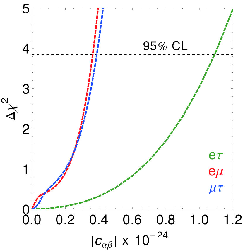
In Fig. 3, we display the expected 95% C.L. sensitivity regions for the case of the DUNE setup in the and planes, left and right panel, respectively. We have marginalized over the corresponding LIV phases and from [0], as well as the atmospheric mixing angle and the leptonic phase , considering a 1 uncertainty of 10% and 15% around their NO best-fit values, as displayed in Table 1. It is observed that flavor-changing LIV coefficients from the () and () sectors may be constrained approximately three times more effectively by the DUNE configuration than by those from the () sector, namely , and , all limits at 95% C.L.


In Fig. 4, we show in left (right) panel, the projected 95% C.L. sensitivities to the SME coefficients and , considering the DUNE configuration. We have marginalized over the corresponding LIV phases from [0], as well as the atmospheric mixing angle and the leptonic phase , considering a 1 uncertainty of 10% and 15%, accordingly. We observe that the sensitivities in the sector , are not as competitive as those from the isotropic and spatial sectors , and , as illustrated in the left and right panels of Fig. 1. Which can be partially understood from their functional dependence in the Hamiltonian of LIV (Eq. 39)
| (44) |
Besides, the null observation of Lorentz violation employing the low-energy excess data set of the MiniBooNE experiment set Katori (2010), while bounds from the Double Chooz experiment constraint Re Katori and Spitz (2014); Kostelecky and Russell (2011).
| LIV sector | Limit (Sensitivity) | Interaction energy scale |
|---|---|---|
| neutrino | , IceCube Abbasi et al. (2022) | |
| neutrino | , Super-Kamiokande Abe et al. (2015) | |
| neutrino | , Super-Kamiokande Abe et al. (2015) | |
| neutrino | , MiniBooNE Katori (2010); Kostelecky and Russell (2011) | |
| neutrino | Re, Double Chooz Katori and Spitz (2014) | |
| neutrino | (), DUNE Raikwal et al. (2023); Agarwalla et al. (2023) | |
| neutrino | (), DUNE (this work) | |
| neutrino | (), DUNE (this work) | |
| neutrino | Re, IceCube Abbasi et al. (2022) | |
| neutrino | Re, IceCube Abbasi et al. (2022) | |
| neutrino | (), DUNE (this work) | |
| neutrino | (), DUNE (this work) | |
| neutrino | (), DUNE (this work) | |
| neutrino | (), DUNE (this work) | |
| electron | Kostelecky and Russell (2011) |
V Conclusions
In contemporary cosmology, one of the most fascinating puzzles are the dark matter and dark energy conundrum. One of the most common fields employed to describe dark energy is the scalar field. Furthermore, a scalar field can also characterize ultralight dark matter, which is one of the most promising alternatives for dark matter.
On the other hand, if the and Lorentz symmetries are broken at very high energies, well beyond the electroweak scale, oscillations of high energy neutrinos may probe energy scales where this possible violations arise. The aforementioned violation of Lorentz invariance might arise from neutrino non-standard interactions with scalar fields.
In this paper, we have outlined the case of an effective tensorial neutrino–scalar field interaction. The corresponding scalar field could be identified as either a dark energy or dark matter candidate. Moreover, within this framework, the effective neutrino interaction with cosmological scalar fields can be associated to the even SME coefficients via the energy momentum-tensor (Sec. III). In the case of the isotropic coefficients , a simple relation can be established in terms of the energy densities () for DE or DM (Eq. 27). Therefore, bounds and sensitivities set on the even SME coefficients () may be related to the energy scale () of this interaction.
Furthermore, we estimate sensitivities to the dimension-four even SME coefficients of the SME, particularly the isotropic and spatial . For an accelerator-based experiment similar to DUNE, our predicted sensitivities at 95% C.L. are (left panel of Fig. 1) and (right panel of Fig. 1), while for the diagonal LIV coefficients and (left panel of Fig. 2); and (right panel of Fig. 2). Our results are summarized in Table 2.
Upcoming and present neutrino experiments such as the DUNE, KM3NeT, IceCube-Gen2 and GRAND proposals; as well as the IceCube neutrino observatory, could shed more light on these types of neutrino interactions.
This paper represents the views of the authors and should not be considered a DUNE collaboration paper.
Acknowledgments
This work was partially supported by SNII-México and CONAHCyT research Grant No. A1-S-23238. Additionally the work of R. C. was partially supported by COFAA-IPN, Estímulos al Desempeño de los Investigadores (EDI)-IPN and SIP-IPN Grant No. 20241624.
Appendix A Details of a tensorial neutrino interaction
A possible realization of the tensorial coupling discussed in this work could arise from conformal coupling and disformal transformations where the scalar field couples to different kinds of matter fields in the form Gauthier et al. (2010); Brax (2012); Brax and Burrage (2014); Carrillo González et al. (2021); Yazdani Ahmadabadi and Mohseni Sadjadi (2024, 2022)
| (45) |
where is the determinant of the metric and the disformal transformation can be written as Bekenstein (1993); Deffayet and Garcia-Saenz (2020); Zumalacárregui and García-Bellido (2014)
| (46) |
Disformal transformations have been applied to a wide range of topics in cosmology, from inflation Kaloper (2004) through dark matter Bekenstein (2004), dark energy Zumalacarregui et al. (2010) and its cosmological implications van de Bruck et al. (2013). Besides, disformal transformations have been applied in generalized Palatini gravities Olmo et al. (2009), and it has been studied their possible non-trivial effects on radiation and signatures in laboratory tests Brax et al. (2012). Following the construction presented in Brax (2012); Brax and Burrage (2014) we can decompose the transformation in the following form 888In fact, there are more general disformal transformations akin Ikeda et al. (2023), where , . The functions depend on the variables , where and . However, the consistency of the fermionic coupling requires that Takahashi et al. (2023).
| (47) |
where is related to energy scale of the interaction. Considering the term as a small correction to , we can expand the action at first order and obtain a derivative coupling of the scalar field with matter
| (48) |
where the sum considers different matter components and is the energy momentum tensor of the matter fields. In the case of fermions
| (49) |
and the energy-momentum tensor is
| (50) |
Therefore, the interaction term can be written as
| (51) |
It is convenient to select a particular choice of the and functions to construct the energy-momentum tensor for the scalar field in the interaction
| (52) |
The effective Lagrangian has a similar structure that appears in modified gravity Asimakis et al. (2023) where there is a coupling of the energy-momentum tensor with the Einstein tensor and a proposal of a coupling among the energy-momentum tensor and vector and scalar fields Beltrán Jiménez et al. (2018). Moreover, a similar interaction was proposed in Refs. Kehagias (2011); Ciuffoli et al. (2013) in the context of Galileonneutrino couplings. For neutrinos, the interaction term can be written as
| (53) |
In cases where the Minkowski metric () is a good approximation, the former relation reduces to
| (54) |
References
- Riess et al. (1998) A. G. Riess et al. (Supernova Search Team), Astron. J. 116, 1009 (1998), arXiv:astro-ph/9805201 .
- Perlmutter et al. (1999) S. Perlmutter et al. (Supernova Cosmology Project), Astrophys. J. 517, 565 (1999), arXiv:astro-ph/9812133 .
- Sahni (2004) V. Sahni, Lect. Notes Phys. 653, 141 (2004), arXiv:astro-ph/0403324 .
- Alam et al. (2004) U. Alam, V. Sahni, and A. A. Starobinsky, JCAP 06, 008 (2004), arXiv:astro-ph/0403687 .
- Adame et al. (2024) A. G. Adame et al. (DESI), (2024), arXiv:2404.03002 [astro-ph.CO] .
- Arbey and Mahmoudi (2021) A. Arbey and F. Mahmoudi, Prog. Part. Nucl. Phys. 119, 103865 (2021), arXiv:2104.11488 [hep-ph] .
- Magana and Matos (2012) J. Magana and T. Matos, J. Phys. Conf. Ser. 378, 012012 (2012), arXiv:1201.6107 [astro-ph.CO] .
- Ferreira (2021) E. G. M. Ferreira, Astron. Astrophys. Rev. 29, 7 (2021), arXiv:2005.03254 [astro-ph.CO] .
- Suárez et al. (2014) A. Suárez, V. H. Robles, and T. Matos, Astrophys. Space Sci. Proc. 38, 107 (2014), arXiv:1302.0903 [astro-ph.CO] .
- Hui et al. (2017) L. Hui, J. P. Ostriker, S. Tremaine, and E. Witten, Phys. Rev. D 95, 043541 (2017), arXiv:1610.08297 [astro-ph.CO] .
- Matos et al. (2024) T. Matos, L. A. Ureña López, and J.-W. Lee, Front. Astron. Space Sci. 11, 1347518 (2024), arXiv:2312.00254 [astro-ph.CO] .
- Arvanitaki et al. (2010) A. Arvanitaki, S. Dimopoulos, S. Dubovsky, N. Kaloper, and J. March-Russell, Phys. Rev. D 81, 123530 (2010), arXiv:0905.4720 [hep-th] .
- Cicoli et al. (2022) M. Cicoli, V. Guidetti, N. Righi, and A. Westphal, JHEP 05, 107 (2022), arXiv:2110.02964 [hep-th] .
- Acharya et al. (2010) B. S. Acharya, K. Bobkov, and P. Kumar, JHEP 11, 105 (2010), arXiv:1004.5138 [hep-th] .
- Marsh (2016) D. J. E. Marsh, Phys. Rept. 643, 1 (2016), arXiv:1510.07633 [astro-ph.CO] .
- Arvanitaki et al. (2015) A. Arvanitaki, J. Huang, and K. Van Tilburg, Phys. Rev. D 91, 015015 (2015), arXiv:1405.2925 [hep-ph] .
- Arvanitaki et al. (2016) A. Arvanitaki, S. Dimopoulos, and K. Van Tilburg, Phys. Rev. Lett. 116, 031102 (2016), arXiv:1508.01798 [hep-ph] .
- Arvanitaki et al. (2018) A. Arvanitaki, P. W. Graham, J. M. Hogan, S. Rajendran, and K. Van Tilburg, Phys. Rev. D 97, 075020 (2018), arXiv:1606.04541 [hep-ph] .
- Li et al. (2011) M. Li, X.-D. Li, S. Wang, and Y. Wang, Commun. Theor. Phys. 56, 525 (2011), arXiv:1103.5870 [astro-ph.CO] .
- Wetterich (1988) C. Wetterich, Nucl. Phys. B 302, 668 (1988), arXiv:1711.03844 [hep-th] .
- Zlatev et al. (1999) I. Zlatev, L.-M. Wang, and P. J. Steinhardt, Phys. Rev. Lett. 82, 896 (1999), arXiv:astro-ph/9807002 .
- (22) C. Käding, Astronomy 2 (2023) no.2, 128-140 doi:10.3390/astronomy2020009 [arXiv:2304.05875 [astro-ph.CO]].
- (23) C. Burrage, E. J. Copeland, C. Käding and P. Millington, Phys. Rev. D 99 (2019) no.4, 043539 doi:10.1103/PhysRevD.99.043539 [arXiv:1811.12301 [astro-ph.CO]].
- Chiba et al. (2000) T. Chiba, T. Okabe, and M. Yamaguchi, Phys. Rev. D 62, 023511 (2000), arXiv:astro-ph/9912463 .
- Armendariz-Picon et al. (2000) C. Armendariz-Picon, V. F. Mukhanov, and P. J. Steinhardt, Phys. Rev. Lett. 85, 4438 (2000), arXiv:astro-ph/0004134 .
- Armendariz-Picon et al. (2001) C. Armendariz-Picon, V. F. Mukhanov, and P. J. Steinhardt, Phys. Rev. D 63, 103510 (2001), arXiv:astro-ph/0006373 .
- Melchiorri et al. (2003) A. Melchiorri, L. Mersini-Houghton, C. J. Odman, and M. Trodden, Phys. Rev. D 68, 043509 (2003), arXiv:astro-ph/0211522 .
- Chiba (2002) T. Chiba, Phys. Rev. D 66, 063514 (2002), arXiv:astro-ph/0206298 .
- Chimento and Feinstein (2004) L. P. Chimento and A. Feinstein, Mod. Phys. Lett. A 19, 761 (2004), arXiv:astro-ph/0305007 .
- Chimento (2004) L. P. Chimento, Phys. Rev. D 69, 123517 (2004), arXiv:astro-ph/0311613 .
- Armendariz-Picon et al. (1999) C. Armendariz-Picon, T. Damour, and V. F. Mukhanov, Phys. Lett. B 458, 209 (1999), arXiv:hep-th/9904075 .
- Garriga and Mukhanov (1999) J. Garriga and V. F. Mukhanov, Phys. Lett. B 458, 219 (1999), arXiv:hep-th/9904176 .
- Scherrer (2004) R. J. Scherrer, Phys. Rev. Lett. 93, 011301 (2004), arXiv:astro-ph/0402316 .
- de Putter and Linder (2007) R. de Putter and E. V. Linder, Astropart. Phys. 28, 263 (2007), arXiv:0705.0400 [astro-ph] .
- Gao and Yang (2010) X.-T. Gao and R.-J. Yang, Phys. Lett. B 687, 99 (2010), arXiv:1003.2786 [gr-qc] .
- Nicolis et al. (2009) A. Nicolis, R. Rattazzi, and E. Trincherini, Phys. Rev. D 79, 064036 (2009), arXiv:0811.2197 [hep-th] .
- de Rham and Tolley (2010) C. de Rham and A. J. Tolley, JCAP 05, 015 (2010), arXiv:1003.5917 [hep-th] .
- Goon et al. (2011a) G. L. Goon, K. Hinterbichler, and M. Trodden, Phys. Rev. D 83, 085015 (2011a), arXiv:1008.4580 [hep-th] .
- Goon et al. (2011b) G. Goon, K. Hinterbichler, and M. Trodden, JCAP 07, 017 (2011b), arXiv:1103.5745 [hep-th] .
- Deffayet et al. (2010) C. Deffayet, O. Pujolas, I. Sawicki, and A. Vikman, JCAP 10, 026 (2010), arXiv:1008.0048 [hep-th] .
- Pujolas et al. (2011) O. Pujolas, I. Sawicki, and A. Vikman, JHEP 11, 156 (2011), arXiv:1103.5360 [hep-th] .
- Kimura and Yamamoto (2011) R. Kimura and K. Yamamoto, JCAP 04, 025 (2011), arXiv:1011.2006 [astro-ph.CO] .
- Maity (2013) D. Maity, Phys. Lett. B 720, 389 (2013), arXiv:1209.6554 [hep-th] .
- Weinberg (2008) S. Weinberg, Cosmology (Oxford University Press, 2008).
- Berlin (2016) A. Berlin, Phys. Rev. Lett. 117, 231801 (2016), arXiv:1608.01307 [hep-ph] .
- de Salas et al. (2016) P. F. de Salas, R. A. Lineros, and M. Tórtola, Phys. Rev. D 94, 123001 (2016), arXiv:1601.05798 [astro-ph.HE] .
- Krnjaic et al. (2018) G. Krnjaic, P. A. N. Machado, and L. Necib, Phys. Rev. D 97, 075017 (2018), arXiv:1705.06740 [hep-ph] .
- Brdar et al. (2018) V. Brdar, J. Kopp, J. Liu, P. Prass, and X.-P. Wang, Phys. Rev. D 97, 043001 (2018), arXiv:1705.09455 [hep-ph] .
- Smirnov and Xu (2019) A. Y. Smirnov and X.-J. Xu, JHEP 12, 046 (2019), arXiv:1909.07505 [hep-ph] .
- Dev et al. (2021) A. Dev, P. A. N. Machado, and P. Martínez-Miravé, JHEP 01, 094 (2021), arXiv:2007.03590 [hep-ph] .
- Losada et al. (2022) M. Losada, Y. Nir, G. Perez, and Y. Shpilman, JHEP 04, 030 (2022), arXiv:2107.10865 [hep-ph] .
- Losada et al. (2023) M. Losada, Y. Nir, G. Perez, I. Savoray, and Y. Shpilman, JHEP 03, 032 (2023), arXiv:2205.09769 [hep-ph] .
- Huang et al. (2022) G.-y. Huang, M. Lindner, P. Martínez-Miravé, and M. Sen, Phys. Rev. D 106, 033004 (2022), arXiv:2205.08431 [hep-ph] .
- Cordero et al. (2023) R. Cordero, L. A. Delgadillo, and O. G. Miranda, Phys. Rev. D 107, 075023 (2023), arXiv:2207.11308 [hep-ph] .
- Sen and Smirnov (2024) M. Sen and A. Y. Smirnov, JCAP 01, 040 (2024), arXiv:2306.15718 [hep-ph] .
- Barranco et al. (2011) J. Barranco, O. G. Miranda, C. A. Moura, T. I. Rashba, and F. Rossi-Torres, JCAP 10, 007 (2011), arXiv:1012.2476 [astro-ph.CO] .
- Reynoso and Sampayo (2016) M. M. Reynoso and O. A. Sampayo, Astropart. Phys. 82, 10 (2016), arXiv:1605.09671 [hep-ph] .
- Gu et al. (2007) P.-H. Gu, X.-J. Bi, and X.-m. Zhang, Eur. Phys. J. C 50, 655 (2007), arXiv:hep-ph/0511027 .
- Ando et al. (2009) S. Ando, M. Kamionkowski, and I. Mocioiu, Phys. Rev. D 80, 123522 (2009), arXiv:0910.4391 [hep-ph] .
- Klop and Ando (2018) N. Klop and S. Ando, Phys. Rev. D 97, 063006 (2018), arXiv:1712.05413 [hep-ph] .
- Capozzi et al. (2018) F. Capozzi, I. M. Shoemaker, and L. Vecchi, JCAP 07, 004 (2018), arXiv:1804.05117 [hep-ph] .
- Farzan and Palomares-Ruiz (2019) Y. Farzan and S. Palomares-Ruiz, Phys. Rev. D 99, 051702 (2019), arXiv:1810.00892 [hep-ph] .
- Ge and Murayama (2019) S.-F. Ge and H. Murayama, (2019), arXiv:1904.02518 [hep-ph] .
- Gherghetta and Shkerin (2023) T. Gherghetta and A. Shkerin, Phys. Rev. D 108, 095009 (2023), arXiv:2305.06441 [hep-ph] .
- Argüelles et al. (2023a) C. A. Argüelles, K. Farrag, and T. Katori, PoS ICRC2023, 1415 (2023a), arXiv:2402.18126 [hep-ph] .
- Argüelles et al. (2023b) C. A. Argüelles, K. Farrag, and T. Katori, in 9th Meeting on CPT and Lorentz Symmetry (2023) arXiv:2401.15716 [hep-ph] .
- Lambiase and Poddar (2024) G. Lambiase and T. K. Poddar, JCAP 01, 069 (2024), arXiv:2307.05229 [hep-ph] .
- Cordero and Delgadillo (2024) R. Cordero and L. A. Delgadillo, Phys. Lett. B 853, 138687 (2024), arXiv:2312.16320 [hep-ph] .
- Argüelles et al. (2024) C. A. Argüelles, K. Farrag, and T. Katori, (2024), arXiv:2404.10926 [hep-ph] .
- Kostelecky and Mewes (2004a) V. A. Kostelecky and M. Mewes, Phys. Rev. D 69, 016005 (2004a), arXiv:hep-ph/0309025 .
- Diaz (2016) J. S. Diaz, Symmetry 8, 105 (2016), arXiv:1609.09474 [hep-ph] .
- Torri (2020) M. D. C. Torri, Universe 6, 37 (2020), arXiv:2110.09186 [hep-ph] .
- Moura and Rossi-Torres (2022) C. A. Moura and F. Rossi-Torres, Universe 8, 42 (2022).
- Barenboim (2022) G. Barenboim, Front. in Phys. 10, 813753 (2022).
- Colladay and Kostelecky (1998) D. Colladay and V. A. Kostelecky, Phys. Rev. D 58, 116002 (1998), arXiv:hep-ph/9809521 .
- Barenboim and Lykken (2003) G. Barenboim and J. D. Lykken, Phys. Lett. B 554, 73 (2003), arXiv:hep-ph/0210411 .
- Barenboim et al. (2019) G. Barenboim, M. Masud, C. A. Ternes, and M. Tórtola, Phys. Lett. B 788, 308 (2019), arXiv:1805.11094 [hep-ph] .
- Abbasi et al. (2022) R. Abbasi et al. (IceCube), Nature Phys. 18, 1287 (2022), arXiv:2111.04654 [hep-ex] .
- Sahoo et al. (2022) S. Sahoo, A. Kumar, and S. K. Agarwalla, JHEP 03, 050 (2022), arXiv:2110.13207 [hep-ph] .
- Agarwalla et al. (2023) S. K. Agarwalla, S. Das, S. Sahoo, and P. Swain, JHEP 07, 216 (2023), arXiv:2302.12005 [hep-ph] .
- Raikwal et al. (2023) D. Raikwal, S. Choubey, and M. Ghosh, Phys. Rev. D 107, 115032 (2023), arXiv:2303.10892 [hep-ph] .
- (82) A. Crivellin, F. Kirk and M. Schreck, JHEP 04 (2021), 082 doi:10.1007/JHEP04(2021)082 [arXiv:2009.01247 [hep-ph]].
- Testagrossa et al. (2023) F. Testagrossa, D. F. G. Fiorillo, and M. Bustamante, (2023), arXiv:2310.12215 [astro-ph.HE] .
- (84) S. Shukla, S. Mishra, L. Singh and V. Singh, [arXiv:2408.01520 [hep-ph]].
- Díaz et al. (2020) F. N. Díaz, J. Hoefken, and A. M. Gago, Phys. Rev. D 102, 055020 (2020), arXiv:2003.13712 [hep-ph] .
- Barenboim and Mavromatos (2005) G. Barenboim and N. E. Mavromatos, JHEP 01, 034 (2005), arXiv:hep-ph/0404014 .
- De Romeri et al. (2023) V. De Romeri, C. Giunti, T. Stuttard, and C. A. Ternes, JHEP 09, 097 (2023), arXiv:2306.14699 [hep-ph] .
- Barenboim and Gago (2024) G. Barenboim and A. M. Gago, (2024), arXiv:2402.03438 [hep-ph] .
- (89) L. A. Delgadillo, O. G. Miranda, G. Moreno-Granados and C. A. Moura, [arXiv:2409.03716 [hep-ph]].
- Abi et al. (2020a) B. Abi et al. (DUNE), (2020a), arXiv:2002.03005 [hep-ex] .
- Antonelli et al. (2018) V. Antonelli, L. Miramonti, and M. D. C. Torri, Eur. Phys. J. C 78, 667 (2018), arXiv:1803.08570 [hep-ph] .
- (92) C. M. Reyes, C. Riquelme and A. Soto, [arXiv:2407.13041 [gr-qc]].
- (93) J. V. V. Santos and M. Schreck, [arXiv:2407.20688 [gr-qc]].
- Gauthier et al. (2010) C. S. Gauthier, R. Saotome, and R. Akhoury, JHEP 07, 062 (2010), arXiv:0911.3168 [hep-ph] .
- Khalifeh and Jimenez (2021a) A. R. Khalifeh and R. Jimenez, Phys. Dark Univ. 31, 100777 (2021a), arXiv:2010.08181 [gr-qc] .
- Khalifeh and Jimenez (2021b) A. R. Khalifeh and R. Jimenez, Phys. Dark Univ. 34, 100897 (2021b), arXiv:2105.07973 [astro-ph.CO] .
- Khalifeh and Jimenez (2022) A. R. Khalifeh and R. Jimenez, Phys. Dark Univ. 37, 101063 (2022), arXiv:2111.15249 [astro-ph.CO] .
- Huang and Nath (2018) G.-Y. Huang and N. Nath, Eur. Phys. J. C 78, 922 (2018), arXiv:1809.01111 [hep-ph] .
- de Salas et al. (2019) P. F. de Salas, K. Malhan, K. Freese, K. Hattori, and M. Valluri, JCAP 10, 037 (2019), arXiv:1906.06133 [astro-ph.GA] .
- de Salas and Widmark (2021) P. F. de Salas and A. Widmark, Rept. Prog. Phys. 84, 104901 (2021), arXiv:2012.11477 [astro-ph.GA] .
- Sivertsson et al. (2022) S. Sivertsson, J. I. Read, H. Silverwood, P. F. de Salas, K. Malhan, A. Widmark, C. F. P. Laporte, S. Garbari, and K. Freese, Mon. Not. Roy. Astron. Soc. 511, 1977 (2022), arXiv:2201.01822 [astro-ph.GA] .
- Kostelecky and Russell (2011) V. A. Kostelecky and N. Russell, Rev. Mod. Phys. 83, 11 (2011), arXiv:0801.0287 [hep-ph] .
- Brax and Burrage (2014) P. Brax and C. Burrage, Phys. Rev. D 90, 104009 (2014), arXiv:1407.1861 [astro-ph.CO] .
- Telalovic and Bustamante (2023) B. Telalovic and M. Bustamante, (2023), arXiv:2310.15224 [astro-ph.HE] .
- Abi et al. (2020b) B. Abi et al. (DUNE), Eur. Phys. J. C 80, 978 (2020b), arXiv:2006.16043 [hep-ex] .
- Huber et al. (2005) P. Huber, M. Lindner, and W. Winter, Comput. Phys. Commun. 167, 195 (2005), arXiv:hep-ph/0407333 [hep-ph] .
- Huber et al. (2007) P. Huber, J. Kopp, M. Lindner, M. Rolinec, and W. Winter, Comput. Phys. Commun. 177, 432 (2007), arXiv:hep-ph/0701187 [hep-ph] .
- Kopp (2008) J. Kopp, Int. J. Mod. Phys. C 19, 523 (2008), arXiv:physics/0610206 .
- Kopp et al. (2007) J. Kopp, M. Lindner, T. Ota, and J. Sato, in 15th International Conference on Supersymmetry and the Unification of Fundamental Interactions (SUSY07) (2007) pp. 756–759, arXiv:0710.1867 [hep-ph] .
- Abi et al. (2021) B. Abi et al. (DUNE), (2021), arXiv:2103.04797 [hep-ex] .
- Kostelecky and Mewes (2004b) V. A. Kostelecky and M. Mewes, Phys. Rev. D 70, 076002 (2004b), arXiv:hep-ph/0406255 .
- Diaz et al. (2009) J. S. Diaz, V. A. Kostelecky, and M. Mewes, Phys. Rev. D 80, 076007 (2009), arXiv:0908.1401 [hep-ph] .
- Mishra et al. (2023) S. Mishra, S. Shukla, L. Singh, and V. Singh, (2023), arXiv:2309.01756 [hep-ph] .
- Huber et al. (2002) P. Huber, M. Lindner, and W. Winter, Nucl. Phys. B 645, 3 (2002), arXiv:hep-ph/0204352 .
- de Salas et al. (2021) P. F. de Salas, D. V. Forero, S. Gariazzo, P. Martínez-Miravé, O. Mena, C. A. Ternes, M. Tórtola, and J. W. F. Valle, JHEP 02, 071 (2021), arXiv:2006.11237 [hep-ph] .
- Abe et al. (2015) K. Abe et al. (Super-Kamiokande), Phys. Rev. D 91, 052003 (2015), arXiv:1410.4267 [hep-ex] .
- Katori (2010) T. Katori (MiniBooNE), in 5th Meeting on CPT and Lorentz Symmetry (2010) pp. 70–74, arXiv:1008.0906 [hep-ph] .
- Katori and Spitz (2014) T. Katori and J. Spitz, in 6th Meeting on CPT and Lorentz Symmetry (2014) pp. 9–12, arXiv:1307.5805 [hep-ph] .
- Brax (2012) P. Brax, Phys. Lett. B 712, 155 (2012), arXiv:1202.0740 [hep-ph] .
- Carrillo González et al. (2021) M. Carrillo González, Q. Liang, J. Sakstein, and M. Trodden, JCAP 04, 063 (2021), arXiv:2011.09895 [astro-ph.CO] .
- Yazdani Ahmadabadi and Mohseni Sadjadi (2024) H. Yazdani Ahmadabadi and H. Mohseni Sadjadi, Phys. Lett. B 850, 138493 (2024), arXiv:2201.02927 [hep-ph] .
- Yazdani Ahmadabadi and Mohseni Sadjadi (2022) H. Yazdani Ahmadabadi and H. Mohseni Sadjadi, (2022), arXiv:2209.13367 [hep-ph] .
- Bekenstein (1993) J. D. Bekenstein, Phys. Rev. D 48, 3641 (1993), arXiv:gr-qc/9211017 .
- Deffayet and Garcia-Saenz (2020) C. Deffayet and S. Garcia-Saenz, Phys. Rev. D 102, 064037 (2020), arXiv:2004.11619 [hep-th] .
- Zumalacárregui and García-Bellido (2014) M. Zumalacárregui and J. García-Bellido, Phys. Rev. D 89, 064046 (2014), arXiv:1308.4685 [gr-qc] .
- Kaloper (2004) N. Kaloper, Phys. Lett. B 583, 1 (2004), arXiv:hep-ph/0312002 .
- Bekenstein (2004) J. D. Bekenstein, Phys. Rev. D 70, 083509 (2004), [Erratum: Phys.Rev.D 71, 069901 (2005)], arXiv:astro-ph/0403694 .
- Zumalacarregui et al. (2010) M. Zumalacarregui, T. S. Koivisto, D. F. Mota, and P. Ruiz-Lapuente, JCAP 05, 038 (2010), arXiv:1004.2684 [astro-ph.CO] .
- van de Bruck et al. (2013) C. van de Bruck, J. Morrice, and S. Vu, Phys. Rev. Lett. 111, 161302 (2013), arXiv:1303.1773 [astro-ph.CO] .
- Olmo et al. (2009) G. J. Olmo, H. Sanchis-Alepuz, and S. Tripathi, Phys. Rev. D 80, 024013 (2009), arXiv:0907.2787 [gr-qc] .
- Brax et al. (2012) P. Brax, C. Burrage, and A.-C. Davis, Journal of Cosmology and Astroparticle Physics 2012, 016 (2012).
- Ikeda et al. (2023) T. Ikeda, K. Takahashi, and T. Kobayashi, Phys. Rev. D 108, 044006 (2023), arXiv:2302.03418 [gr-qc] .
- Takahashi et al. (2023) K. Takahashi, R. Kimura, and H. Motohashi, Phys. Rev. D 107, 044018 (2023), arXiv:2212.13391 [gr-qc] .
- Asimakis et al. (2023) P. Asimakis, S. Basilakos, A. Lymperis, M. Petronikolou, and E. N. Saridakis, Phys. Rev. D 107, 104006 (2023), arXiv:2212.03821 [gr-qc] .
- Beltrán Jiménez et al. (2018) J. Beltrán Jiménez, J. A. R. Cembranos, and J. M. Sánchez Velázquez, JHEP 05, 100 (2018), arXiv:1803.05832 [hep-th] .
- Kehagias (2011) A. Kehagias, (2011), arXiv:1109.6312 [hep-ph] .
- Ciuffoli et al. (2013) E. Ciuffoli, J. Evslin, J. Liu, and X. Zhang, ISRN High Energy Phys. 2013, 497071 (2013), arXiv:1109.6641 [hep-ph] .