NeuS: Learning Neural Implicit Surfaces
by Volume Rendering for Multi-view Reconstruction
Abstract
We present a novel neural surface reconstruction method, called NeuS, for reconstructing objects and scenes with high fidelity from 2D image inputs. Existing neural surface reconstruction approaches, such as DVR [Niemeyer et al., 2020] and IDR [Yariv et al., 2020], require foreground mask as supervision, easily get trapped in local minima, and therefore struggle with the reconstruction of objects with severe self-occlusion or thin structures. Meanwhile, recent neural methods for novel view synthesis, such as NeRF [Mildenhall et al., 2020] and its variants, use volume rendering to produce a neural scene representation with robustness of optimization, even for highly complex objects. However, extracting high-quality surfaces from this learned implicit representation is difficult because there are not sufficient surface constraints in the representation. In NeuS, we propose to represent a surface as the zero-level set of a signed distance function (SDF) and develop a new volume rendering method to train a neural SDF representation. We observe that the conventional volume rendering method causes inherent geometric errors (i.e. bias) for surface reconstruction, and therefore propose a new formulation that is free of bias in the first order of approximation, thus leading to more accurate surface reconstruction even without the mask supervision. Experiments on the DTU dataset and the BlendedMVS dataset show that NeuS outperforms the state-of-the-arts in high-quality surface reconstruction, especially for objects and scenes with complex structures and self-occlusion.
1 Introduction
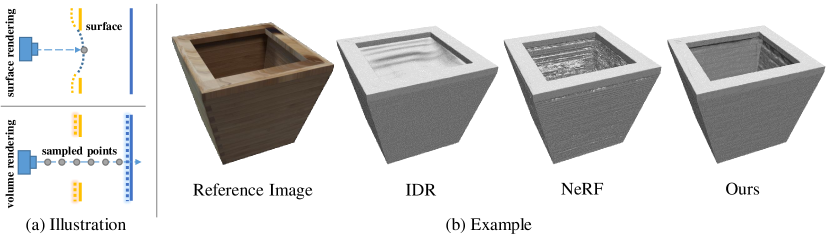
Reconstructing surfaces from multi-view images is a fundamental problem in computer vision and computer graphics. 3D reconstruction with neural implicit representations has recently become a highly promising alternative to classical reconstruction approaches [37, 8, 2] due to its high reconstruction quality and its potential to reconstruct complex objects that are difficult for classical approaches, such as non-Lambertian surfaces and thin structures. Recent works represent surfaces as signed distance functions (SDF) [49, 52, 17, 23] or occupancy [30, 31]. To train their neural models, these methods use a differentiable surface rendering method to render a 3D object into images and compare them against input images for supervision. For example, IDR [49] produces impressive reconstruction results, but it fails to reconstruct objects with complex structures that causes abrupt depth changes. The cause of this limitation is that the surface rendering method used in IDR only considers a single surface intersection point for each ray. Consequently, the gradient only exists at this single point, which is too local for effective back propagation and would get optimization stuck in a poor local minimum when there are abrupt changes of depth on images. Furthermore, object masks are needed as supervision for converging to a valid surface. As illustrated in Fig. 1 (a) top, with the radical depth change caused by the hole, the neural network would incorrectly predict the points near the front surface to be blue, failing to find the far-back blue surface. The actual test example in Fig. 1 (b) shows that IDR fails to correctly reconstruct the surfaces near the edges with abrupt depth changes.
Recently, NeRF [29] and its variants have explored to use a volume rendering method to learn a volumetric radiance field for novel view synthesis. This volume rendering approach samples multiple points along each ray and perform -composition of the colors of the sampled points to produce the output pixel colors for training purposes. The advantage of the volume rendering approach is that it can handle abrupt depth changes, because it considers multiple points along the ray and so all the sample points, either near the surface or on the far surface, produce gradient signals for back propagation. For example, referring Fig. 1 (a) bottom, when the near surface (yellow) is found to have inconsistent colors with the input image, the volume rendering approach is capable of training the network to find the far-back surface to produce the correct scene representation. However, since it is intended for novel view synthesis rather than surface reconstruction, NeRF only learns a volume density field, from which it is difficult to extract a high-quality surface. Fig. 1 (b) shows a surface extracted as a level-set surface of the density field learned by NeRF. Although the surface correctly accounts for abrupt depth changes, it contains conspicuous noise in some planar regions.
In this work, we present a new neural rendering scheme, called NeuS, for multi-view surface reconstruction. NeuS uses the signed distance function (SDF) for surface representation and uses a novel volume rendering scheme to learn a neural SDF representation. Specifically, by introducing a density distribution induced by SDF, we make it possible to apply the volume rendering approach to learning an implicit SDF representation and thus have the best of both worlds, i.e. an accurate surface representation using a neural SDF model and robust network training in the presence of abrupt depth changes as enabled by volume rendering. Note that simply applying a standard volume rendering method to the density associated with SDF would lead to discernible bias (i.e. inherent geometric errors) in the reconstructed surfaces. This is a new and important observation that we will elaborate later. Therefore we propose a novel volume rendering scheme to ensure unbiased surface reconstruction in the first-order approximation of SDF. Experiments on both DTU dataset and BlendedMVS dataset demonstrated that NeuS is capable of reconstructing complex 3D objects and scenes with severe occlusions and delicate structures, even without foreground masks as supervision. It outperforms the state-of-the-art neural scene representation methods, namely IDR [49] and NeRF [29], in terms of reconstruction quality.
2 Related Works
Classical Multi-view Surface and Volumetric Reconstruction. Traditional multi-view 3D reconstruction methods can be roughly classified into two categories: point- and surface-based reconstruction [2, 8, 9, 37] and volumetric reconstruction [6, 3, 38]. Point- and surface-based reconstruction methods estimate the depth map of each pixel by exploiting inter-image photometric consistency [8] and then fuse the depth maps into a global dense point cloud [26, 51]. The surface reconstruction is usually done as a post processing with methods like screened Poisson surface reconstruction [16]. The reconstruction quality heavily relies on the quality of correspondence matching, and the difficulties in matching correspondence for objects without rich textures often lead to severe artifacts and missing parts in the reconstruction results. Alternatively, volumetric reconstruction methods circumvent the difficulty of explicit correspondence matching by estimating occupancy and color in a voxel grid from multi-view images and evaluating the color consistency of each voxel. Due to limited achievable voxel resolution, these methods cannot achieve high accuracy.
Neural Implicit Representation. Some methods enforce 3D understanding in a deep learning framework by introducing inductive biases. These inductive biases can be explicit representations, such as voxel grids [13, 5, 47], point cloud [7, 25, 19], meshes [44, 46, 14], and implicit representations. The implicit representations encoded by a neural network has gained a lot of attention recently, since it is continuous and can achieve high spatial resolution. This representation has been applied successfully to shape representation [27, 28, 32, 4, 1, 10, 50, 33], novel view synthesis [40, 24, 15, 29, 22, 34, 35, 43, 39] and multi-view 3D reconstruction [49, 30, 17, 12, 23].
Our work mainly focuses on learning implicit neural representation encoding both geometry and appearance in 3D space from 2D images via classical rendering techniques. Limited in this scope, the related works can be roughly categorized based on the rendering techniques used, i.e. surface rendering based methods and volume rendering based methods. Surface rendering based methods [30, 17, 49, 23] assume that the color of ray only relies on the color of an intersection of the ray with the scene geometry, which makes the gradient only backpropagated to a local region near the intersection. Therefore, such methods struggle with reconstructing complex objects with severe self-occlusions and sudden depth changes. Furthermore, they usually require object masks as supervision. On the contrary, our method performs well for such challenging cases without the need of masks.
Volume rendering based methods, such as NeRF[29], render an image by -compositing colors of the sampled points along each ray. As explained in the introduction, it can handle sudden depth changes and synthesize high-quality images. However, extracting high-fidelity surface from the learned implicit field is difficult because the density-based scene representation lacks sufficient constraints on its level sets. In contrast, our method combines the advantages of surface rendering based and volume rendering based methods by constraining the scene space as a signed distance function but applying volume rendering to train this representation with robustness. UNISURF [31], a concurrent work, also learns an implicit surface via volume rendering. It improves the reconstruction quality by shrinking the sample region of volume rendering during the optimization. Our method differs from UNISURF in that UNISURF represents the surface by occupancy values, while our method represents the scene by an SDF and thus can naturally extract the surface as the zero-level set of it, yielding better reconstruction accuracy than UNISURF, as will be seen later in the experiment section.
3 Method
Given a set of posed images of a 3D object, our goal is to reconstruct the surface of it. The surface is represented by the zero-level set of a neural implicit SDF. In order to learn the weights of the neural network, we developed a novel volume rendering method to render images from the implicit SDF and minimize the difference between the rendered images and the input images. This volume rendering approach ensures robust optimization in NeuS for reconstructing objects of complex structures.
3.1 Rendering Procedure
Scene representation. With NeuS, the scene of an object to be reconstructed is represented by two functions: that maps a spatial position to its signed distance to the object, and that encodes the color associated with a point and a viewing direction . Both functions are encoded by Multi-layer Perceptrons (MLP). The surface of the object is represented by the zero-level set of its SDF, that is,
| (1) |
In order to apply a volume rendering method to training the SDF network, we first introduce a probability density function , called S-density, where , , is the signed distance function and , commonly known as the logistic density distribution, is the derivative of the Sigmoid function , i.e., . In principle can be any unimodal (i.e. bell-shaped) density distribution centered at ; here we choose the logistic density distribution for its computational convenience. Note that the standard deviation of is given by , which is also a trainable parameter, that is, approaches to zero as the network training converges.
Intuitively, the main idea of NeuS is that, with the aid of the S-density field , volume rendering is used to train the SDF network with only 2D input images as supervision. Upon successful minimization of a loss function based on this supervision, the zero-level set of the network-encoded SDF is expected to represent an accurately reconstructed surface , with its induced S-density assuming prominently high values near the surface.
Rendering. To learn the parameters of the neural SDF and color field, we advise a volume rendering scheme to render images from the proposed SDF representation. Given a pixel, we denote the ray emitted from this pixel as , where is the center of the camera and is the unit direction vector of the ray. We accumulate the colors along the ray by
| (2) |
where is the output color for this pixel, a weight for the point , and the color at the point along the viewing direction .
Requirements on weight function. The key to learn an accurate SDF representation from 2D images is to build an appropriate connection between output colors and SDF, i.e., to derive an appropriate weight function on the ray based on the SDF of the scene. In the following, we list the requirements on the weight function .
-
1.
Unbiased. Given a camera ray , attains a locally maximal value at a surface intersection point , i.e. with , that is, the point is on the zero-level set of the SDF .
-
2.
Occlusion-aware. Given any two depth values and satisfying , , , and , there is . That is, when two points have the same SDF value (thus the same SDF-induced S-density value), the point nearer to the view point should have a larger contribution to the final output color than does the other point.
An unbiased weight function guarantees that the intersection of the camera ray with the zero-level set of SDF contributes most to the pixel color. The occlusion-aware property ensures that when a ray sequentially passes multiple surfaces, the rendering procedure will correctly use the color of the surface nearest to the camera to compute the output color.
Next, we will first introduce a naive way of defining the weight function that directly using the standard pipeline of volume rendering, and explain why it is not appropriate for reconstruction before introducing our novel construction of .
Naive solution. To make the weight function occlusion-aware, a natural solution is based on the standard volume rendering formulation [29] which defines the weight function by
| (3) |
where is the so-called volume density in classical volume rendering and here denotes the accumulated transmittance along the ray. To adopt the standard volume density formulation [29], here is set to be equal to the S-density value, i.e. and the weight function is computed by Eqn. 3. Although the resulting weight function is occlusion-aware, it is biased as it introduces inherent errors in the reconstructed surfaces. As illustrated in Fig. 2 (a), the weight function attains a local maximum at a point before the ray reaches the surface point , satisfying . This fact will be proved in the supplementary material.
Our solution. To introduce our solution, we first introduce a straightforward way to construct an unbiased weight function, which directly uses the normalized S-density as weights
| (4) |
This construction of weight function is unbiased, but not occlusion-aware. For example, if the ray penetrates two surfaces, the SDF function will have two zero points on the ray, which leads to two peaks on the weight function and the resulting weight function will equally blend the colors of two surfaces without considering occlusions.
To this end, now we shall design the weight function that is both occlusion-aware and unbiased in the first-order approximation of SDF, based on the aforementioned straightforward construction. To ensure an occlusion-aware property of the weight function , we will still follow the basic framework of volume rendering as Eqn. 3. However, different from the conventional treatment as in naive solution above, we define our function from the S-density in a new manner. We first define an opaque density function , which is the counterpart of the volume density in standard volume rendering. Then we compute the new weight function by
| (5) |
How we derive opaque density . We first consider a simple ideal case where there is only one surface intersection, and the surface is simply a plane that approaches infinitely far off the camera. Since Eqn. 4 indeed satisfies the above requirements under this assumption, we derive the underlying opaque density corresponding to the weight definition of Eqn. 4 using the framework of volume rendering. Then we will generalize this opaque density to the general case of multiple surface intersections.
Specifically, in the simple case of a single plane intersection, it is easy to see that the signed distance function is , where , and is the angle between the view direction and the outward surface normal vector . Because the surface is assumed a plane, is a constant. It follows from Eqn. 4 that
| (6) |
Recall that the weight function within the framework of volume rendering is given by , where denotes the accumulated transmittance. Therefore, to derive , we have
| (7) |
Since , it is easy to verify that . Further, note that . It follows that . Integrating both sides of this equation yields
| (8) |
Taking the logarithm and then differentiating both sides, we have
| (9) |
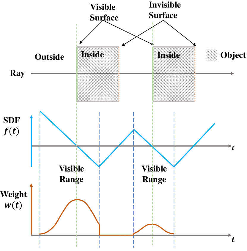
This is the formula of the opaque density in the ideal case of single plane intersection. The weight function induced by is shown in Figure 2(b). Now we generalize the opaque density to the general case where there are multiple surface intersections along the ray . In this case, becomes negative on the segment of the ray with increasing SDF values. Thus we clip it against zero to ensure that the value of is always non-negative. This gives the following opaque density function in general cases.
| (10) |
Based on this equation, the weight function can be computed with standard volume rendering as in Eqn. 5. The illustration in the case of multiple surface intersection is shown in Figure 3.
The following theorem states that in general cases (i.e., including both single surface intersection and multiple surface intersections) the weight function defined by Eqn. 10 and Eqn. 5 is unbiased in the first-order approximation of SDF. The proof is given in the supplementary material.
Theorem 1
Suppose that a smooth surface is defined by the zero-level set of the signed distance function , and a ray enters the surface from outside to inside, with the intersection point at , that is, and there exists an interval such that and is monotonically decreasing in . Suppose that in this local interval , the surface can be tangentially approximated by a sufficiently small planar patch, i.e., is regarded as fixed. Then, the weight function computed by Eqn. 10 and Eqn. 5 in attains its maximum at .
Discretization. To obtain discrete counterparts of the opacity and weight function, we adopt the same approximation scheme as used in NeRF [29], This scheme samples points along the ray to compute the approximate pixel color of the ray as
| (11) |
where is the discrete accumulated transmittance defined by , and is discrete opacity values defined by
| (12) |
which can further be shown to be
| (13) |
The detailed derivation of this formula for is given in the supplementary material.
3.2 Training
To train NeuS, we minimize the difference between the rendered colors and the ground truth colors, without any 3D supervision. Besides colors, we can also utilize the masks for supervision if provided.
Specifically, we optimize our neural networks and inverse standard deviation by randomly sampling a batch of pixels and their corresponding rays in world space , where is its pixel color and is its optional mask value, from an image in every iteration. We assume the point sampling size is and the batch size is . The loss function is defined as
| (14) |
The color loss is defined as
| (15) |
Same as IDR[49], we empirically choose as L1 loss, which in our observation is robust to outliers and stable in training.
We add an Eikonal term [10] on the sampled points to regularize the SDF of by
| (16) |
The optional mask loss is defined as
| (17) |
where is the sum of weights along the camera ray, and BCE is the binary cross entropy loss.
Hierarchical sampling. In this work, we follow a similar hierarchical sampling strategy as in NeRF [29]. We first uniformly sample the points on the ray and then iteratively conduct importance sampling on top of the coarse probability estimation. The difference is that, unlike NeRF which simultaneously optimizes a coarse network and a fine network, we only maintain one network, where the probability in coarse sampling is computed based on the S-density with fixed standard deviations while the probability of fine sampling is computed based on with the learned . Details of hierarchical sampling strategy are provided in supplementary materials.
Scan 24
(DTU)
Scan 37
(DTU)

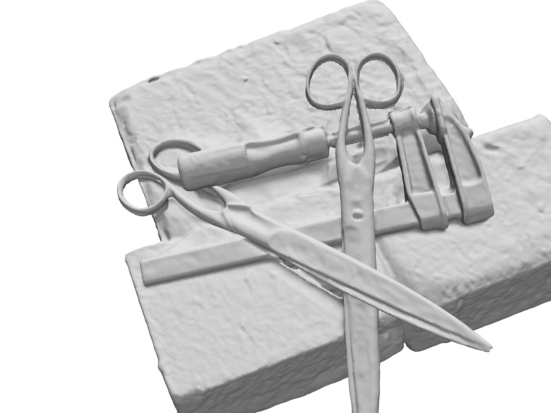
Dog
(BlendedMVS)
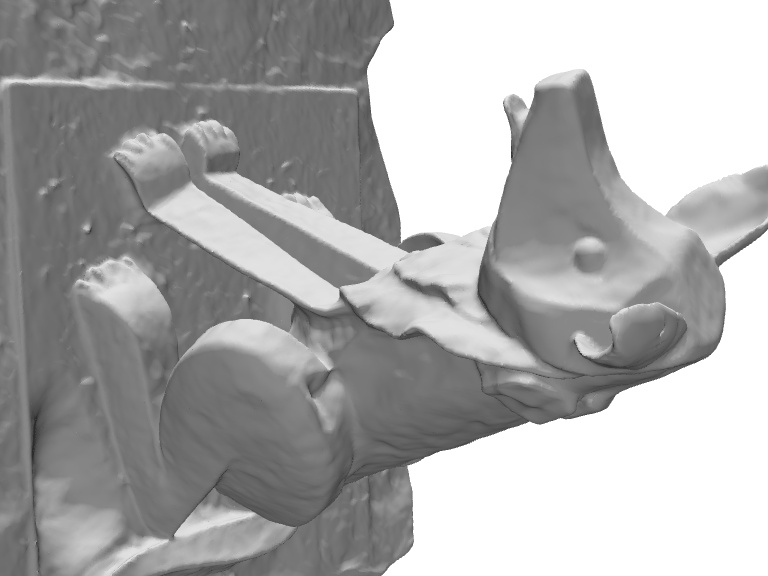
Stone
(BlendedMVS)
Reference Image
Ours
IDR
NeRF
4 Experiments
4.1 Experimental settings
Datasets. To evaluate our approach and baseline methods, we use 15 scenes from the DTU dataset [11], same as those used in IDR [49], with a wide variety of materials, appearance and geometry, including challenging cases for reconstruction algorithms, such as non-Lambertian surfaces and thin structures. Each scene contains 49 or 64 images with the image resolution of . Each scene was tested with and without foreground masks provided by IDR [49]. We further tested on 7 challenging scenes from the low-res set of the BlendedMVS dataset [48](CC-4 License). Each scene has images at pixels and masks are provided by the BlendedMVS dataset. We further captured two thin objects with 32 input images to test our approach on thin structure reconstruction.
Baselines. (1) The state-of-the-art surface rendering approach – IDR [49]: IDR can reconstruct surface with high quality but requires foreground masks as supervision; Since IDR has demonstrated superior quality compared to another surface rendering based method – DVR [30], we did not conduct a comparison with DVR. (2) The state-of-the-art volume rendering approach – NeRF [29]: We use a threshold of 25 to extract mesh from the learned density field. We validate this choice in the supplementary material. (3) A widely-used classical MVS method – COLMAP [37]: We reconstruct a mesh from the output point cloud of COLMAP with Screened Poisson Surface Reconstruction [16]. (4) The concurrent work which unifies surface rendering and volume rendering with an occupancy field as scene representation – UNISURF [31]. More details of the baseline methods are included in the supplementary material.
[b] w/ mask w/o mask ScanID IDR NeRF Ours COLMAP NeRF UNISURF Ours scan24 1.63 1.83 0.83 0.81 1.90 1.32 1.00 scan37 1.87 2.39 0.98 2.05 1.60 1.36 1.37 scan40 0.63 1.79 0.56 0.73 1.85 1.72 0.93 scan55 0.48 0.66 0.37 1.22 0.58 0.44 0.43 scan63 1.04 1.79 1.13 1.79 2.28 1.35 1.10 scan65 0.79 1.44 0.59 1.58 1.27 0.79 0.65 scan69 0.77 1.50 0.60 1.02 1.47 0.80 0.57 scan83 1.33 1.20 1.45 3.05 1.67 1.49 1.48 scan97 1.16 1.96 0.95 1.40 2.05 1.37 1.09 scan105 0.76 1.27 0.78 2.05 1.07 0.89 0.83 scan106 0.67 1.44 0.52 1.00 0.88 0.59 0.52 scan110 0.90 2.61 1.43 1.32 2.53 1.47 1.20 scan114 0.42 1.04 0.36 0.49 1.06 0.46 0.35 scan118 0.51 1.13 0.45 0.78 1.15 0.59 0.49 scan122 0.53 0.99 0.45 1.17 0.96 0.62 0.54 mean 0.90 1.54 0.77 1.36 1.49 1.02 0.84
Implementation details. We assume the region of interest is inside a unit sphere. We sample 512 rays per batch and train our model for 300k iterations for 14 hours (for the ‘w/ mask’ setting) and 16 hours (for the ‘w/o mask’ setting) on a single NVIDIA RTX2080Ti GPU. For the ‘w/o mask’ setting, we model the background by NeRF++ [53]. Our network architecture and initialization scheme are similar to those of IDR [49]. More details of the network architecture and training parameters can be found in the supplementary material.
4.2 Comparisons
We conducted the comparisons in two settings, with mask supervision (w/ mask) and without mask supervision (w/o mask). We measure the reconstruction quality with the Chamfer distances in the same way as UNISURF [31] and IDR [49] and report the scores in Table 1. The results show that our approach outperforms the baseline methods on the DTU dataset in both settings – w/ and w/o mask in terms of the Chamfer distance. Note that the reported scores of IDR in the setting of w/ mask and NeRF and UNISURF in the w/o mask setting are from IDR [49] and UNISURF [31].
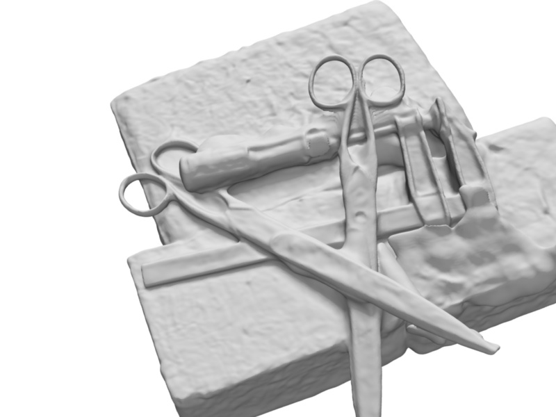
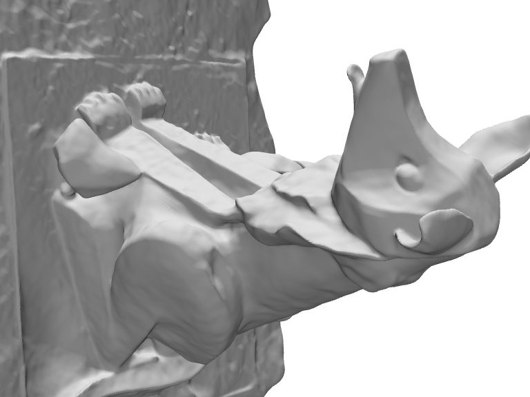
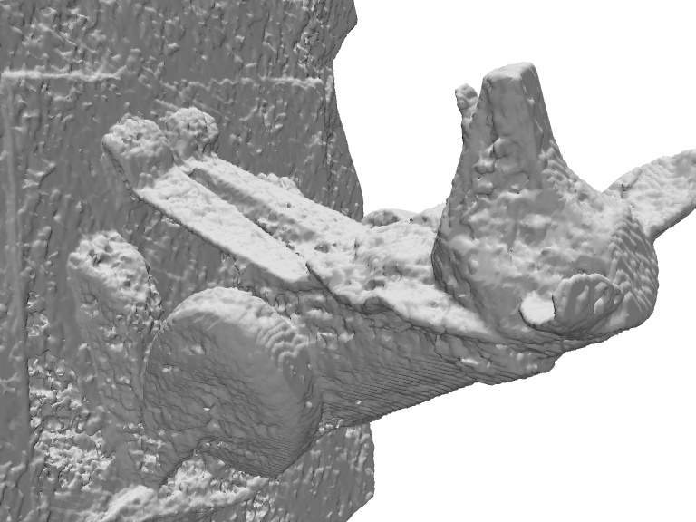
Scan 69
(DTU)
Clock
(BlendedMVS)
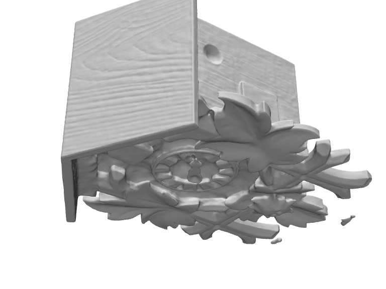
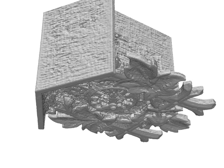
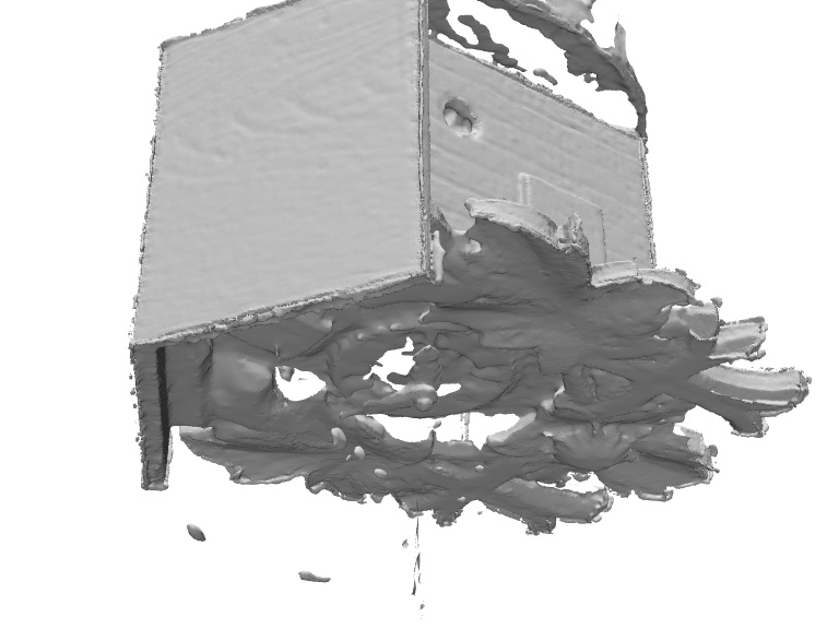
Sculpture
(BlendedMVS)
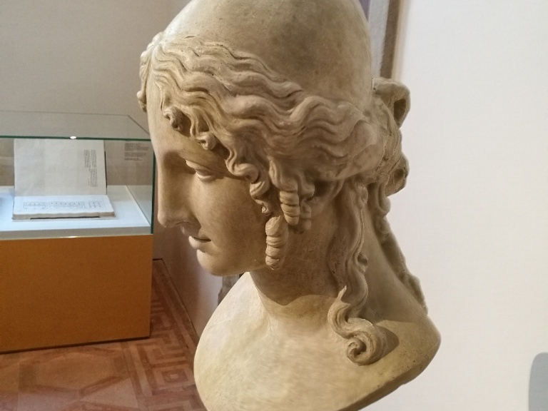
Bear
(BlendedMVS)
Reference Image
Ours
NeRF
COLMAP
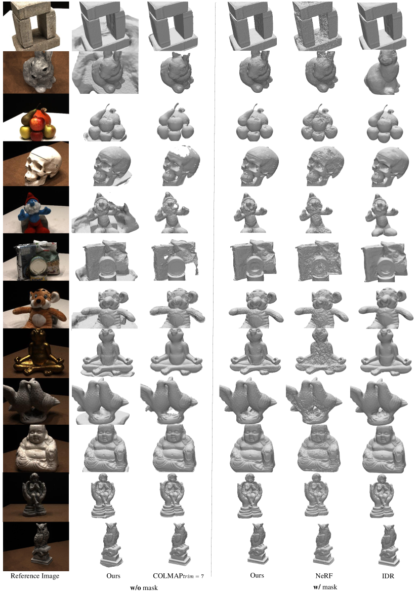
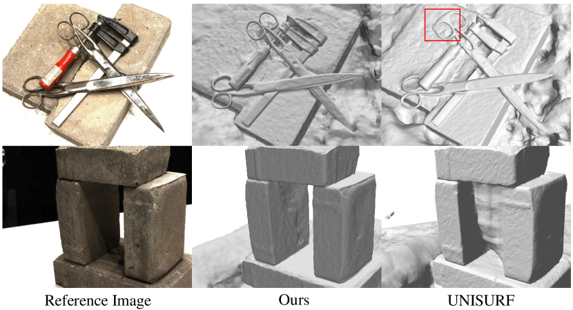
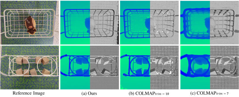
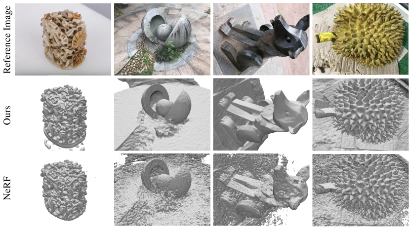
We conduct the qualitative comparisons on the DTU dataset and the BlendedMVS dataset in both settings, w/ mask and w/o mask, in Figure 4 and Figure 5, respectively. As shown in Figure 4 for the setting of w/ mask, IDR shows limited performance for reconstructing thin metals parts in Scan 37 (DTU), and fails to handle sudden depth changes in Stone (BlendedMVS) due to the local optimization process in surface rendering. The extracted meshes of NeRF are noisy since the volume density field has not sufficient constraint on its 3D geometry. Regarding the w/o mask setting, we visually compare our method with NeRF and COLMAP in the setting of w/o mask in Figure 5, which shows our reconstructed surfaces are with more fidelity than baselines. We further show a comparison with UNISURF [31] on two examples in the w/o mask setting. Note that we use the qualitative results of UNISURF reported their paper for comparison. Our method works better for the objects with abrupt depth changes. More qualitative images are included in the supplementary material.
4.3 Analysis
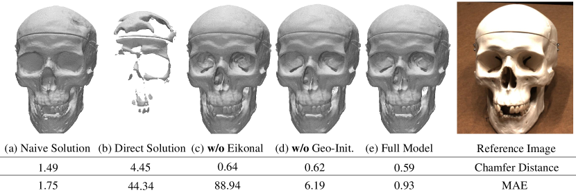
Ablation study.
To evaluate the effect of the weight calculation, we test three different kinds of weight constructions described in Sec. 3.1: (a) Naive Solution. (b) Straightforward Construction as shown in Eqn. 4. (e) Full Model. As shown in Figure 6, the quantitative result of naive solution is worse than our weight choice (e) in terms of the Chamfer distance. This is because it introduces a bias to the surface reconstruction. If direct construction is used, there are severe artifacts.
We also studied the effect of Eikonal regularization [10] and geometric initialization [1]. Without Eikonal regularization or geometric initialization, the result on Chamfer distance is on par with that of the full model. However, neither of them can correctly output a signed distance function. This is indicated by the MAE(mean absolute error) between the SDF predictions and corresponding ground-truth SDF, as shown in the bottom line of Figure 6. The MAE is computed on uniformly-sampled points in the object’s bounding sphere. Qualitative results of SDF predictions are provided in the supplementary material.
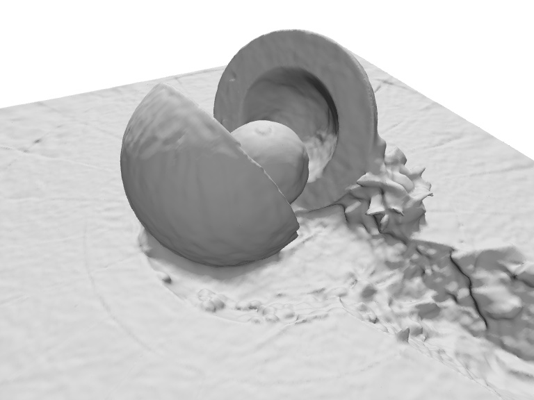
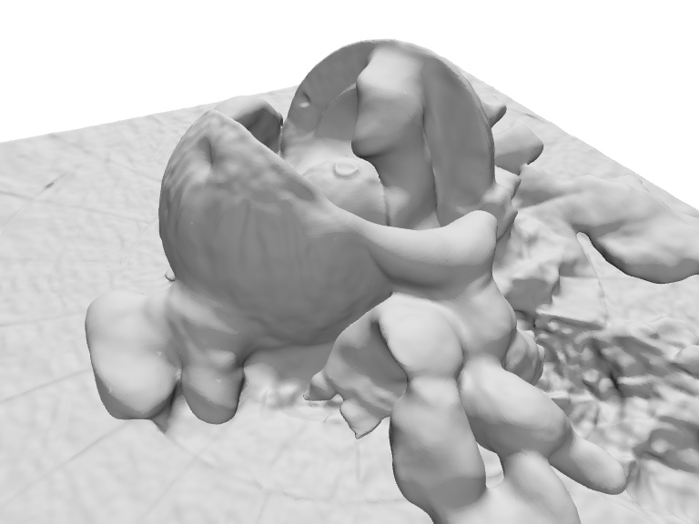
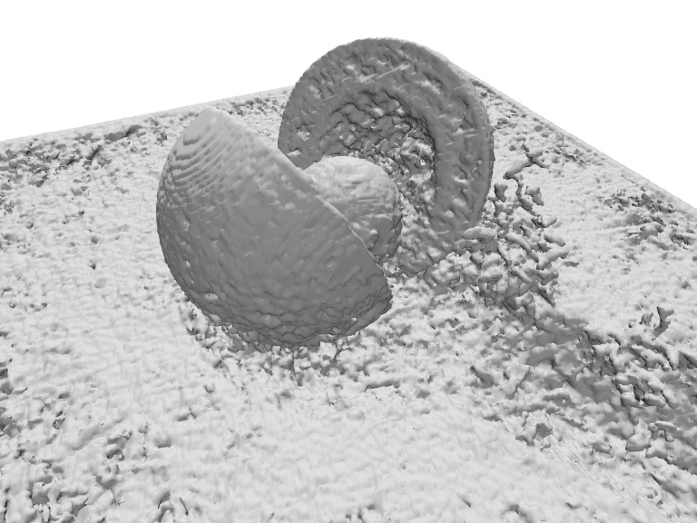
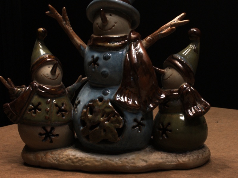
Thin structures. We additionally show results on two challenging thin objects with 32 input images. The plane with rich texture under the object is used for camera calibration. As shown in Fig. 8, our method is able to accurately reconstruct these thin structures, especially on the edges with abrupt depth changes. Furthermore, different from the methods [41, 20, 45, 21] which only target at high-quality thin structure reconstruction, our method can handle the scenes which have a mixture of thin structures and general objects.
5 Conclusion
We have proposed NeuS, a new approach to multiview surface reconstruction that represents 3D surfaces as neural SDF and developed a new volume rendering method for training the implicit SDF representation. NeuS produces high-quality reconstruction and successfully reconstructs objects with severe occlusions and complex structures. It outperforms the state-of-the-arts both qualitatively and quantitatively. One limitation of our method is that although our method does not heavily rely on correspondence matching of texture features, the performance would still degrade for textureless objects (we show the failure cases in the supplementary material). Moreover, NeuS has only a single scale parameter that is used to model the standard deviation of the probability distribution for all the spatial location. Hence, an interesting future research topic is to model the probability with different variances for different spatial locations together with the optimization of scene representation, depending on different local geometric characteristics. Negative societal impact: like many other learning-based works, our method requires a large amount of computational resources for network training, which can be a concern for global climate change.
Acknowlegements
We thank Michael Oechsle for providing the results of UNISURF. Christian Theobalt was supported by ERC Consolidator Grant 770784. Lingjie Liu was supported by Lise Meitner Postdoctoral Fellowship. Computational resources are mainly provided by HKU GPU Farm.
References
- [1] Matan Atzmon and Yaron Lipman. Sal: Sign agnostic learning of shapes from raw data. In Proceedings of the IEEE/CVF Conference on Computer Vision and Pattern Recognition, pages 2565–2574, 2020.
- [2] Connelly Barnes, Eli Shechtman, Adam Finkelstein, and Dan B Goldman. Patchmatch: A randomized correspondence algorithm for structural image editing. ACM Trans. Graph., 28(3):24, 2009.
- [3] Adrian Broadhurst, Tom W Drummond, and Roberto Cipolla. A probabilistic framework for space carving. In Proceedings Eighth IEEE International Conference on Computer Vision. ICCV 2001, volume 1, pages 388–393. IEEE, 2001.
- [4] Z. Chen and H. Zhang. Learning implicit fields for generative shape modeling. In 2019 IEEE/CVF Conference on Computer Vision and Pattern Recognition (CVPR), pages 5932–5941, 2019.
- [5] Christopher B Choy, Danfei Xu, JunYoung Gwak, Kevin Chen, and Silvio Savarese. 3d-r2n2: A unified approach for single and multi-view 3d object reconstruction. In European conference on computer vision, pages 628–644. Springer, 2016.
- [6] Jeremy S De Bonet and Paul Viola. Poxels: Probabilistic voxelized volume reconstruction. In Proceedings of International Conference on Computer Vision (ICCV), pages 418–425, 1999.
- [7] Haoqiang Fan, Hao Su, and Leonidas J Guibas. A point set generation network for 3d object reconstruction from a single image. In Proceedings of the IEEE conference on computer vision and pattern recognition, pages 605–613, 2017.
- [8] Yasutaka Furukawa and Jean Ponce. Accurate, dense, and robust multiview stereopsis. IEEE transactions on pattern analysis and machine intelligence, 32(8):1362–1376, 2009.
- [9] Silvano Galliani, Katrin Lasinger, and Konrad Schindler. Gipuma: Massively parallel multi-view stereo reconstruction. Publikationen der Deutschen Gesellschaft für Photogrammetrie, Fernerkundung und Geoinformation e. V, 25(361-369):2, 2016.
- [10] Amos Gropp, Lior Yariv, Niv Haim, Matan Atzmon, and Yaron Lipman. Implicit geometric regularization for learning shapes. arXiv preprint arXiv:2002.10099, 2020.
- [11] Rasmus Jensen, Anders Dahl, George Vogiatzis, Engil Tola, and Henrik Aanæs. Large scale multi-view stereopsis evaluation. In 2014 IEEE Conference on Computer Vision and Pattern Recognition, pages 406–413, 2014.
- [12] Yue Jiang, Dantong Ji, Zhizhong Han, and Matthias Zwicker. Sdfdiff: Differentiable rendering of signed distance fields for 3d shape optimization. In The IEEE/CVF Conference on Computer Vision and Pattern Recognition (CVPR), June 2020.
- [13] Abhishek Kar, Christian Häne, and Jitendra Malik. Learning a multi-view stereo machine. arXiv preprint arXiv:1708.05375, 2017.
- [14] Hiroharu Kato, Yoshitaka Ushiku, and Tatsuya Harada. Neural 3d mesh renderer. In Proceedings of the IEEE conference on computer vision and pattern recognition, pages 3907–3916, 2018.
- [15] Srinivas Kaza et al. Differentiable volume rendering using signed distance functions. PhD thesis, Massachusetts Institute of Technology, 2019.
- [16] Michael Kazhdan and Hugues Hoppe. Screened poisson surface reconstruction. ACM Trans. Graph., 32(3), July 2013.
- [17] Petr Kellnhofer, Lars Jebe, Andrew Jones, Ryan Spicer, Kari Pulli, and Gordon Wetzstein. Neural lumigraph rendering. arXiv preprint arXiv:2103.11571, 2021.
- [18] Diederik P Kingma and Jimmy Ba. Adam: A method for stochastic optimization. arXiv preprint arXiv:1412.6980, 2014.
- [19] Chen-Hsuan Lin, Chen Kong, and Simon Lucey. Learning efficient point cloud generation for dense 3d object reconstruction. In proceedings of the AAAI Conference on Artificial Intelligence, volume 32, 2018.
- [20] Lingjie Liu, Duygu Ceylan, Cheng Lin, Wenping Wang, and Niloy J. Mitra. Image-based reconstruction of wire art. 36(4):63:1–63:11, 2017.
- [21] Lingjie Liu, Nenglun Chen, Duygu Ceylan, Christian Theobalt, Wenping Wang, and Niloy J. Mitra. Curvefusion: Reconstructing thin structures from rgbd sequences. 37(6), 2018.
- [22] Lingjie Liu, Jiatao Gu, Kyaw Zaw Lin, Tat-Seng Chua, and Christian Theobalt. Neural sparse voxel fields. Advances in Neural Information Processing Systems, 33, 2020.
- [23] Shaohui Liu, Yinda Zhang, Songyou Peng, Boxin Shi, Marc Pollefeys, and Zhaopeng Cui. Dist: Rendering deep implicit signed distance function with differentiable sphere tracing. In Proceedings of the IEEE/CVF Conference on Computer Vision and Pattern Recognition, pages 2019–2028, 2020.
- [24] Stephen Lombardi, Tomas Simon, Jason Saragih, Gabriel Schwartz, Andreas Lehrmann, and Yaser Sheikh. Neural volumes: Learning dynamic renderable volumes from images. ACM Transactions on Graphics (TOG), 38(4):65, 2019.
- [25] Priyanka Mandikal, K L Navaneet, Mayank Agarwal, and R Venkatesh Babu. 3D-LMNet: Latent embedding matching for accurate and diverse 3d point cloud reconstruction from a single image. In Proceedings of the British Machine Vision Conference (BMVC), 2018.
- [26] Paul Merrell, Amir Akbarzadeh, Liang Wang, Philippos Mordohai, Jan-Michael Frahm, Ruigang Yang, David Nistér, and Marc Pollefeys. Real-time visibility-based fusion of depth maps. pages 1–8, 01 2007.
- [27] Lars Mescheder, Michael Oechsle, Michael Niemeyer, Sebastian Nowozin, and Andreas Geiger. Occupancy networks: Learning 3d reconstruction in function space. In Proceedings of the IEEE/CVF Conference on Computer Vision and Pattern Recognition, pages 4460–4470, 2019.
- [28] Mateusz Michalkiewicz, Jhony K. Pontes, Dominic Jack, Mahsa Baktashmotlagh, and Anders Eriksson. Implicit surface representations as layers in neural networks. In The IEEE International Conference on Computer Vision (ICCV), October 2019.
- [29] Ben Mildenhall, Pratul P Srinivasan, Matthew Tancik, Jonathan T Barron, Ravi Ramamoorthi, and Ren Ng. Nerf: Representing scenes as neural radiance fields for view synthesis. In European Conference on Computer Vision, pages 405–421. Springer, 2020.
- [30] Michael Niemeyer, Lars Mescheder, Michael Oechsle, and Andreas Geiger. Differentiable volumetric rendering: Learning implicit 3d representations without 3d supervision. In Proceedings of the IEEE/CVF Conference on Computer Vision and Pattern Recognition, pages 3504–3515, 2020.
- [31] Michael Oechsle, Songyou Peng, and Andreas Geiger. Unisurf: Unifying neural implicit surfaces and radiance fields for multi-view reconstruction. arXiv preprint arXiv:2104.10078, 2021.
- [32] Jeong Joon Park, Peter Florence, Julian Straub, Richard Newcombe, and Steven Lovegrove. Deepsdf: Learning continuous signed distance functions for shape representation. In Proceedings of the IEEE/CVF Conference on Computer Vision and Pattern Recognition, pages 165–174, 2019.
- [33] Songyou Peng, Michael Niemeyer, Lars M. Mescheder, Marc Pollefeys, and Andreas Geiger. Convolutional occupancy networks. ArXiv, abs/2003.04618, 2020.
- [34] Shunsuke Saito, Zeng Huang, Ryota Natsume, Shigeo Morishima, Angjoo Kanazawa, and Hao Li. Pifu: Pixel-aligned implicit function for high-resolution clothed human digitization. ICCV, 2019.
- [35] Shunsuke Saito, Tomas Simon, Jason Saragih, and Hanbyul Joo. Pifuhd: Multi-level pixel-aligned implicit function for high-resolution 3d human digitization. In Proceedings of the IEEE/CVF Conference on Computer Vision and Pattern Recognition, pages 84–93, 2020.
- [36] Tim Salimans and Diederik P Kingma. Weight normalization: A simple reparameterization to accelerate training of deep neural networks. arXiv preprint arXiv:1602.07868, 2016.
- [37] Johannes L Schönberger, Enliang Zheng, Jan-Michael Frahm, and Marc Pollefeys. Pixelwise view selection for unstructured multi-view stereo. In European Conference on Computer Vision, pages 501–518. Springer, 2016.
- [38] Steven M Seitz and Charles R Dyer. Photorealistic scene reconstruction by voxel coloring. International Journal of Computer Vision, 35(2):151–173, 1999.
- [39] Vincent Sitzmann, Justus Thies, Felix Heide, Matthias Nießner, Gordon Wetzstein, and Michael Zollhofer. Deepvoxels: Learning persistent 3d feature embeddings. In Proceedings of the IEEE/CVF Conference on Computer Vision and Pattern Recognition, pages 2437–2446, 2019.
- [40] Vincent Sitzmann, Michael Zollhöfer, and Gordon Wetzstein. Scene representation networks: Continuous 3d-structure-aware neural scene representations. In Advances in Neural Information Processing Systems, pages 1119–1130, 2019.
- [41] A. Tabb. Shape from silhouette probability maps: Reconstruction of thin objects in the presence of silhouette extraction and calibration error. pages 161–168, June 2013.
- [42] Matthew Tancik, Pratul P Srinivasan, Ben Mildenhall, Sara Fridovich-Keil, Nithin Raghavan, Utkarsh Singhal, Ravi Ramamoorthi, Jonathan T Barron, and Ren Ng. Fourier features let networks learn high frequency functions in low dimensional domains. arXiv preprint arXiv:2006.10739, 2020.
- [43] Alex Trevithick and Bo Yang. Grf: Learning a general radiance field for 3d scene representation and rendering. arXiv preprint arXiv:2010.04595, 2020.
- [44] Nanyang Wang, Yinda Zhang, Zhuwen Li, Yanwei Fu, Wei Liu, and Yu-Gang Jiang. Pixel2mesh: Generating 3d mesh models from single rgb images. In Proceedings of the European Conference on Computer Vision (ECCV), pages 52–67, 2018.
- [45] Peng Wang, Lingjie Liu, Nenglun Chen, Hung-Kuo Chu, Christian Theobalt, and Wenping Wang. Vid2curve: Simultaneous camera motion estimation and thin structure reconstruction from an rgb video. ACM Trans. Graph., 39(4), July 2020.
- [46] Chao Wen, Yinda Zhang, Zhuwen Li, and Yanwei Fu. Pixel2mesh++: Multi-view 3d mesh generation via deformation. In Proceedings of the IEEE/CVF International Conference on Computer Vision, pages 1042–1051, 2019.
- [47] Haozhe Xie, Hongxun Yao, Xiaoshuai Sun, Shangchen Zhou, and Shengping Zhang. Pix2vox: Context-aware 3d reconstruction from single and multi-view images. In Proceedings of the IEEE/CVF International Conference on Computer Vision, pages 2690–2698, 2019.
- [48] Yao Yao, Zixin Luo, Shiwei Li, Jingyang Zhang, Yufan Ren, Lei Zhou, Tian Fang, and Long Quan. Blendedmvs: A large-scale dataset for generalized multi-view stereo networks. In Proceedings of the IEEE/CVF Conference on Computer Vision and Pattern Recognition, pages 1790–1799, 2020.
- [49] Lior Yariv, Yoni Kasten, Dror Moran, Meirav Galun, Matan Atzmon, Basri Ronen, and Yaron Lipman. Multiview neural surface reconstruction by disentangling geometry and appearance. Advances in Neural Information Processing Systems, 33, 2020.
- [50] Wang Yifan, Shihao Wu, Cengiz Oztireli, and Olga Sorkine-Hornung. Iso-points: Optimizing neural implicit surfaces with hybrid representations. arXiv preprint arXiv:2012.06434, 2020.
- [51] Christopher Zach, Thomas Pock, and Horst Bischof. A globally optimal algorithm for robust tv-l1 range image integration. In 2007 IEEE 11th International Conference on Computer Vision, pages 1–8, 2007.
- [52] Kai Zhang, Fujun Luan, Qianqian Wang, Kavita Bala, and Noah Snavely. Physg: Inverse rendering with spherical gaussians for physics-based material editing and relighting. arXiv preprint arXiv:2104.00674, 2021.
- [53] Kai Zhang, Gernot Riegler, Noah Snavely, and Vladlen Koltun. Nerf++: Analyzing and improving neural radiance fields. arXiv preprint arXiv:2010.07492, 2020.
- Supplementary -
A Derivation for Computing Opacity
In this section we will derive the formula in Eqn. 13 of the paper for computing the discrete opacity . Recall that the opaque density function is defined as
| (18) |
where and are the probability density function (PDF) and cumulative distribution function (CDF) of logistic distribution, respectively. First consider the case where the sample point interval lies in a range over which the camera ray is entering the surface from outside to inside, i.e. the signed distance function is decreasing on the camera ray over . Then it is easy to see that in . It follows from Eqn. 12 of the paper that,
| (19) |
Note that the integral term is computed by
| (20) |
where is a constant. Thus the discrete opacity can be computed by
| (21) |
Next consider the case where lies in a range over which the camera ray is exiting the surface, i.e. the signed distance function is increasing on over . Then we have in . Then, according to Eqn. 18, we have . Therefore, by Eqn. 12 of the paper, we have
Hence, the alpha value in this case is given by
| (22) |
This completes the derivation of Eqn. 13 of the paper.
B First-order Bias Analysis
B.1 Proof of Unbiased Property of Our Solution
Proof of Theorem 1: Suppose that the ray is going from outside to inside of the surface. Hence, we have , because by convention the signed distance function is positive outside and negative inside of the surface.
Recall that our S-density field is defined using the logistic density function , which is the derivative of the Sigmoid function , i.e. .
According to Eqn. 5 of the paper, the weight function is given by
where
By assumption, for . Since is a probability density function, we have . Clearly, . It follows that
which is positive. Hence,
| (23) |
As a first-order approximation of signed distance function , suppose that locally the surface is tangentially approximated by a sufficiently small planar patch with its outward unit normal vector denoted as . Because is a signed distance function, locally it has a unit gradient vector . Then we have
| (24) |
where is the angle between the view direction and the unit normal vector , that is, . Here can be regarded as a constant. Hence, attains a local maximum when because is a unimodal density function attaining the maximal value at .
We remark that in this proof we do not make any assumption on the existence of surfaces between the camera and the sample point . Therefore the conclusion holds true for the case of multiple surface intersections on the camera ray. This completes the proof.
B.2 Bias in Naive Solution
In this section we show that the weight function derived in naive solution is biased. According to Eqn. 3 of the paper, , with the opacity . Then we have
| (25) |
Now we perform the same first-order approximation of signed distance function near the surface intersection as in Section B.1. In this condition, the above equation can be rewritten as
| (26) |
Here can be regarded as a constant. Now suppose is a point on the surface , that is, . Next we will examine the value of at . First, clearly, and . Then, since , we have
Hence in naive solution does not attain a local maximum at , which corresponds to a point on the surface . This completes the proof.
C Second-order Bias Analysis
In this section we briefly introduce our local analysis in the interval near the surface intersection, in second-order approximation. In this condition, we follow the similar assumption as Section B that the signed distance function monotonically decreases along the ray in the interval .
According to Eqn. 25, the derivative of is given by:
Clearly, we have . Hence, when attains local maximum at , there is .
The case of our solution. In our solution, the volume density is given by following Eqn. 18. After organizing, we have
Here we perform a local analysis at near the surface intersection , where , . And we let , and . As a second-order analysis, we assume that in this local interval , is fixed. After substitution and organization, the induced equation for local maximum point is
| (27) |
which we will analyze later.
The case of the naive solution. Here we conduct a similar local analysis as in case of our solution. Regarding naive solution, when attains local maximum at , there is:
| (28) |
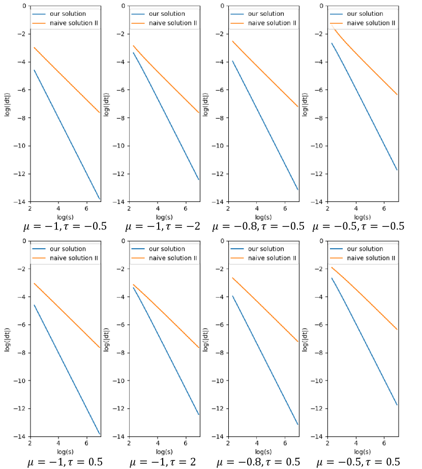
Comparison. Based on Eqn. 27 and Eqn. 28, we can numerically solve the equations on for any given values of and . Below we plot the curves of versus increasing for different (fixed) values of in Fig. 9.
As shown in Fig. 9, the error of local maximum position for our solution and the error for the naive solution. That is to say, our error converges to zero faster than the error of the naive solution does as the standard deviation of the -density approaches to , which is quadratic convergence versus linear convergence.
D Additional Experimental Details
D.1 Additional Implemenation Details
Network architecture. We use a similar network architecture as IDR [49], which consists of two MLPs to encode SDF and color respectively. The signed distance function is modeled by an MLP that consists of 8 hidden layers with hidden size of 256. We replace original ReLU with Softplus with as activation functions for all hidden layers. A skip connection [32] is used to connect the input with the output of the fourth layer. The function for color prediction is modeled by a MLP with 4 hidden layers with size of 256, which takes not only the spatial location as inputs but also the view direction , the normal vector of SDF , and a 256-dimensional feature vector from the SDF MLP. Positional encoding is applied to spatial location with 6 frequencies and to view direction with 4 frequencies. Same as IDR, we use weight normalization [36] to stabilize the training process.
Training details. We train our neural networks using the ADAM optimizer [18]. The learning rate is first linearly warmed up from 0 to in the first 5k iterations, and then controlled by the cosine decay schedule to the minimum learning rate of . We train each model for 300k iterations for 14 hours (for the ‘w/ mask’ setting) and 16 hours (for the ‘w/o mask’ setting) in total on a single Nvidia 2080Ti GPU.
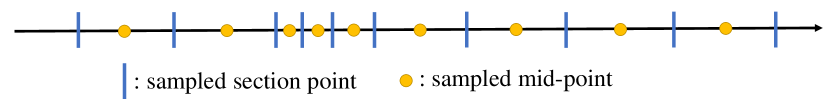
Alpha and color computation. In the implementation, we actually have two types of sampling points - the sampled section points and the sampled mid-points , with section length , as illustrated in Figure 10. To compute the alpha value , we use the section points, which is . To compute the color , we use the color of the mid-point .
Hierarchical sampling. Specifically, we first uniformly sample 64 points along the ray, then we iteratively conduct importance sampling for times. The coarse probability estimation in the i-th iteration is computed by a fixed value, which is set as . In each iteration, we additionally sample 16 points. Therefore, the total number of sampled points for NeuS is 128. For the ‘w/o mask’ setting, we sample extra 32 points outside the sphere. The outside scene is represented using NeRF++ [53].
| Scan ID | Threshold 0 | Threshold 25 | Threshold 50 | Threshold 100 | Threshold 500 |
|---|---|---|---|---|---|
| Scan 40 | 2.36 | 1.79 | 1.86 | 2.07 | 4.26 |
| Scan 83 | 1.65 | 1.20 | 1.37 | 2.24 | 29.10 |
| Scan 114 | 1.62 | 1.04 | 1.10 | 1.43 | 8.66 |
D.2 Baselines
IDR[49]. To implement IDR, we use their officially released codes111https://github.com/lioryariv/idr and pretrained models on the DTU dataset.
NeRF[29]. To implement NeRF, we use the code from nerf-pytorch222https://github.com/yenchenlin/nerf-pytorch. To extract surfaces from NeRF, we use the density level-set of 25, which is validated by experiments to be the best level-set with smallest reconstruction errors, as shown in Table 2 and Figure 11.
COLMAP[37]. We use the officially provided CLI(command line interface) version of COLMAP. Dense point clouds are produced by sequentially running following commands: (1) feature_extractor, (2) exhaustive_matcher, (3) patch_match_stereo, and (4) stereo_fusion. Given dense point clouds, meshes are produced by (5) poisson_mesher.
UNISURF[31]. The quantitative and qualitative results in the paper are provided by the authors of UNISURF.
Threshold 0
Threshold 25
Threshold 50
Threshold 100
Threshold 500
E Additional Experimental Results
|
Scan ID 24 37 40 55 63 65 69 83 97 105 106 110 114 118 122 Mean PSNR(Ours) 28.20 27.10 28.13 28.80 32.05 33.75 30.96 34.47 29.57 32.98 35.07 32.74 31.69 36.97 37.07 31.97 PSNR(OursST) 27.07 26.58 27.70 28.37 31.32 31.39 30.20 31.79 28.58 30.87 33.61 32.40 31.33 35.55 35.96 30.85 SSIM(Ours) 0.764 0.813 0.737 0.768 0.917 0.835 0.845 0.850 0.837 0.837 0.875 0.876 0.861 0.891 0.892 0.840 SSIM(OursST) 0.757 0.811 0.736 0.759 0.915 0.788 0.813 0.812 0.794 0.811 0.852 0.862 0.847 0.867 0.873 0.820 |
|
Scan ID 24 37 40 55 63 65 69 83 97 105 106 110 114 118 122 Mean PSNR(NeRF) 24.83 25.35 26.87 27.64 30.24 29.65 28.03 28.94 26.76 29.61 32.85 31.00 29.94 34.28 33.69 29.31 PSNR(Ours) 23.98 22.79 25.21 26.03 28.32 29.80 27.45 28.89 26.03 28.93 32.47 30.78 29.37 34.23 33.95 28.55 SSIM(NeRF) 0.753 0.794 0.780 0.761 0.915 0.805 0.803 0.822 0.804 0.815 0.870 0.857 0.848 0.880 0.879 0.826 SSIM(Ours) 0.732 0.778 0.722 0.739 0.915 0.809 0.818 0.831 0.812 0.815 0.866 0.863 0.847 0.878 0.878 0.820 |
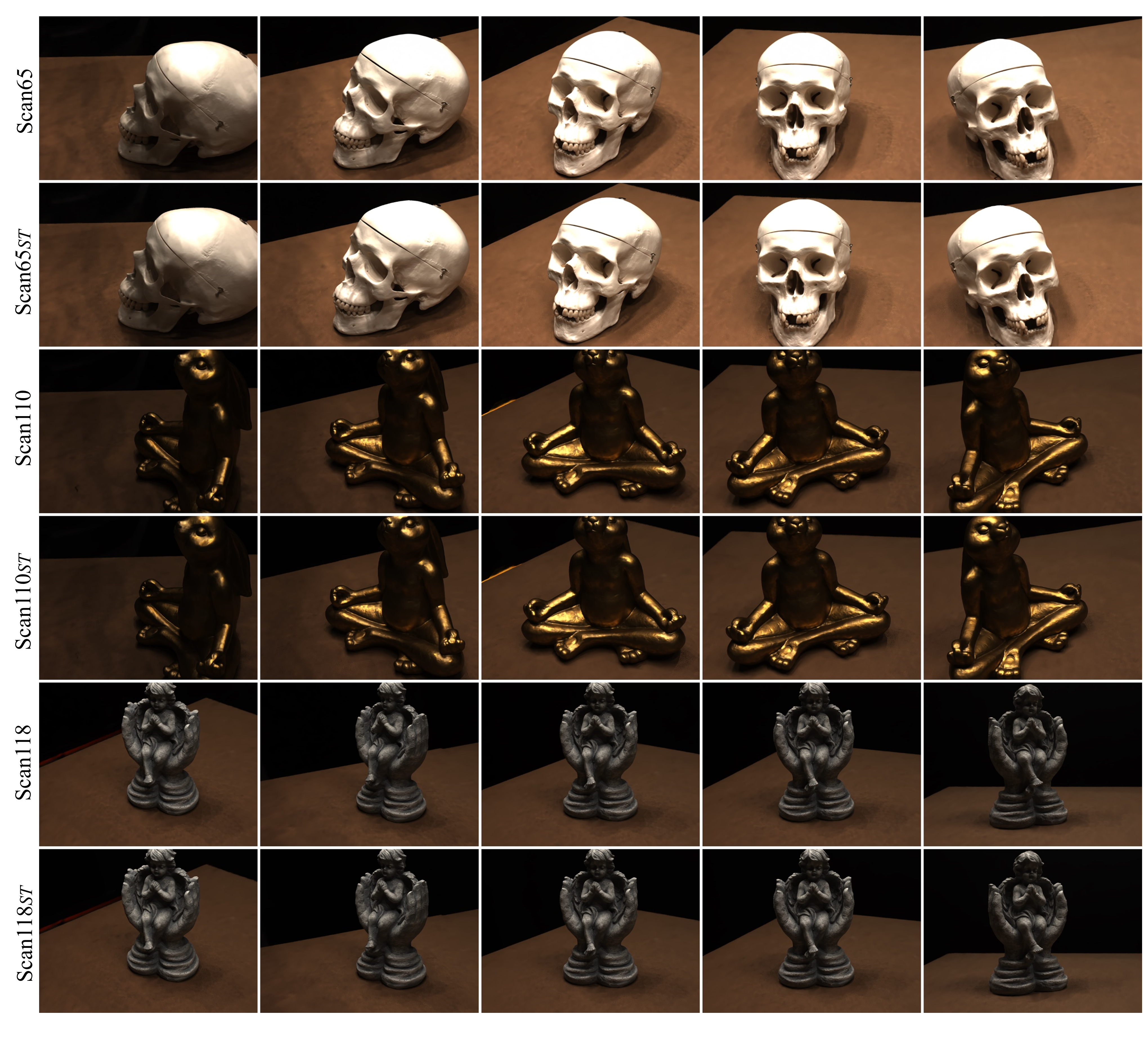
E.1 Rendering Quality and Speed
Besides the reconstructed surfaces, our method also renders high-quality images, as shown in Figure 12. Rendering an image in resolution of 1600x1200 costs about 320 seconds in the default volume rendering setting on a single Nvidia 2080Ti GPU. In addition, we also tested another sampling strategy by first applying sphere tracing to find the regions near the surfaces and only sampling points in those regions. With this strategy, rendering an image in the same resolution only needs about 60 seconds. Table 3 reports the quantitative results in terms of PSNR and SSIM in default volume rendering setting and sphere tracing setting.
E.2 Novel View Synthesis
In this experiment, we held out 10% of the images in the DTU dataset as the testing set and the others as the training set. We compare the quantitative results on the testing set in terms of PSNR and SSIM with NeRF. As shown in Table 4, our method achieves comparable performance to NeRF.
E.3 SDF Qualitative Evaluation
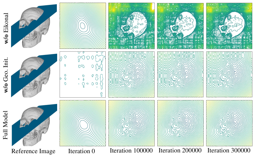
While our method without Eikonal regularization [10] or geometric initialization [1] produces plausible surface reconstruction results, our full model can predict a more accurate signed distance function as shown in Figure 13. Furthermore, using random initialization produces axis-aligned artifacts due to the spectral bias of positional encoding [42] while the geometric initialization [1] does not have such kind of artifacts.
E.4 Training Progression
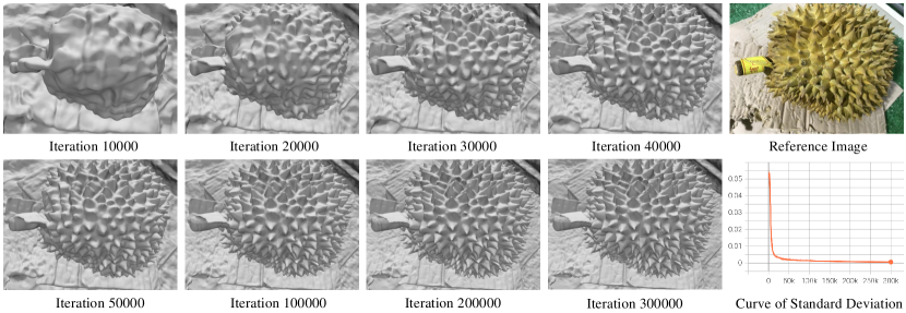
We show the reconstructed surfaces at different training stages of the Durian in the BlendedMVS dataset. As illustrated in Figure 14, the surface gets sharper along the training process. Meanwhile, we also provide a curve in the figure to show how the trainable standard deviation in changes in the training process. As we can see, the optimization process will automatically reduce the standard deviation so that the surface becomes more clear and sharper with more training steps.
E.5 Limitation
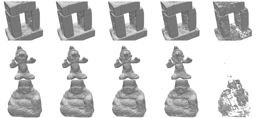
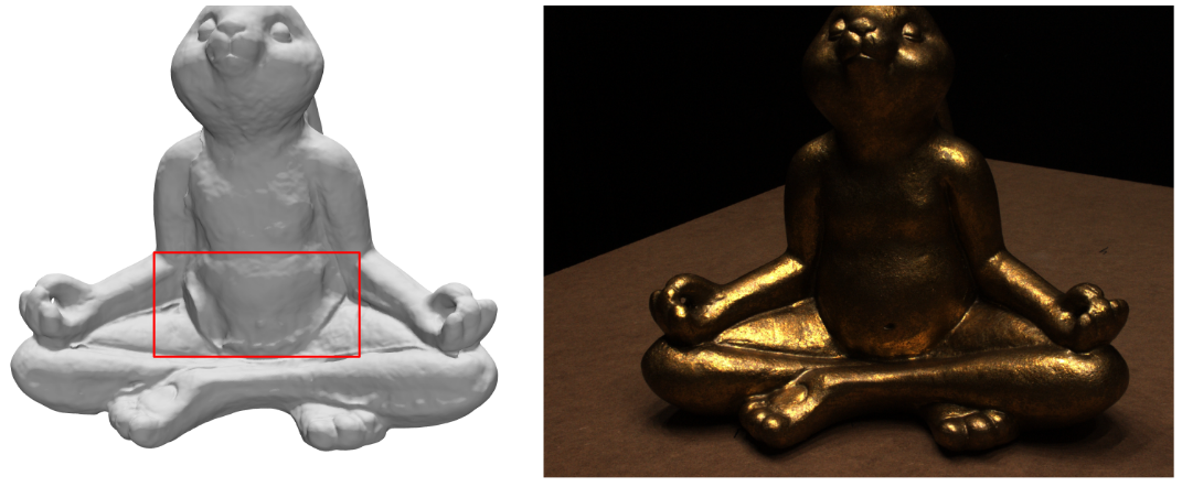
Figure 16 shows a failure case where our method fails to correctly reconstruct the texutreless region of the surface on the metal rabbit model. The reason is that such textureless regions are ambiguous for reconstruction in neural rendering.
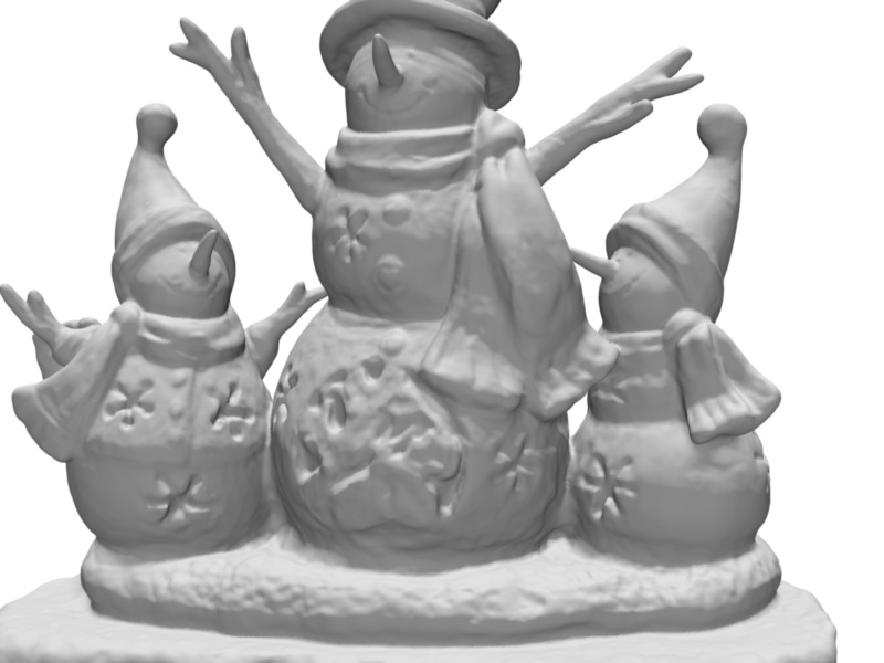
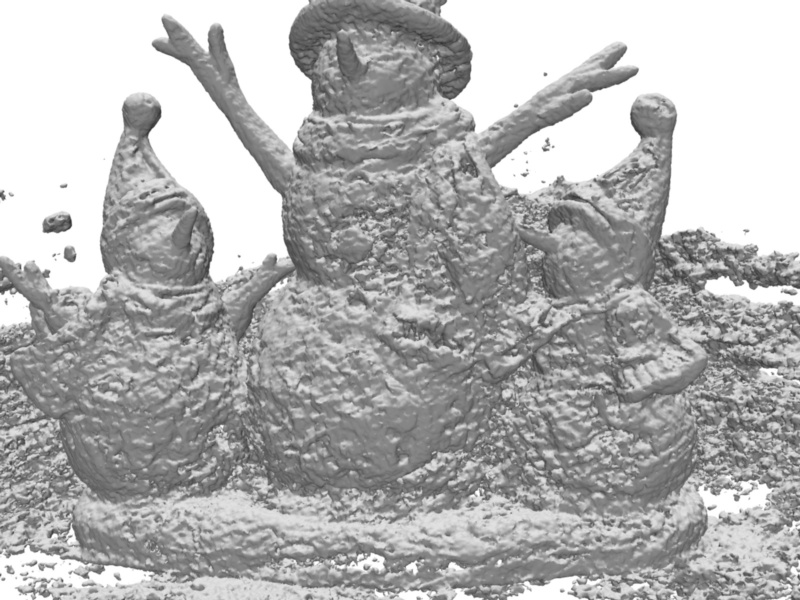
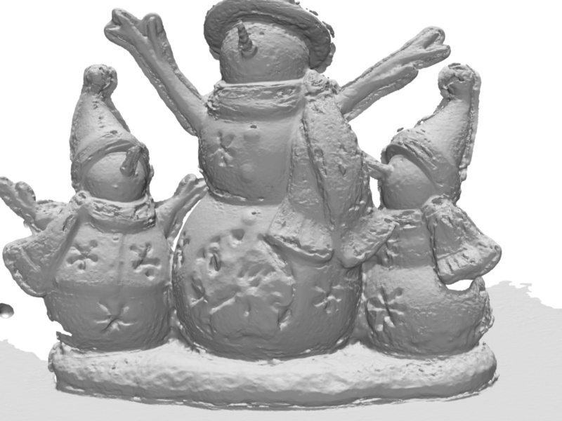
E.6 Additional Results
In this section, we show additional qualitative results on the DTU dataset and BlendedMVS dataset. Figure 17 shows the comparisons with baseline methods in both w/ mask setting and w/o mask setting. Figure 15 shows addtional results in w/o mask setting.