NeuronFair: Interpretable White-Box Fairness Testing through Biased Neuron Identification
Abstract.
Deep neural networks (DNNs) have demonstrated their outperformance in various domains. However, it raises a social concern whether DNNs can produce reliable and fair decisions especially when they are applied to sensitive domains involving valuable resource allocation, such as education, loan, and employment. It is crucial to conduct fairness testing before DNNs are reliably deployed to such sensitive domains, i.e., generating as many instances as possible to uncover fairness violations. However, the existing testing methods are still limited from three aspects: interpretability, performance, and generalizability. To overcome the challenges, we propose NeuronFair, a new DNN fairness testing framework that differs from previous work in several key aspects: (1) interpretable - it quantitatively interprets DNNs’ fairness violations for the biased decision; (2) effective - it uses the interpretation results to guide the generation of more diverse instances in less time; (3) generic - it can handle both structured and unstructured data. Extensive evaluations across 7 datasets and the corresponding DNNs demonstrate NeuronFair’s superior performance. For instance, on structured datasets, it generates much more instances (5.84) and saves more time (with an average speedup of 534.56%) compared with the state-of-the-art methods. Besides, the instances of NeuronFair can also be leveraged to improve the fairness of the biased DNNs, which helps build more fair and trustworthy deep learning systems. The code of NeuronFair is open-sourced at https://github.com/haibinzheng/NeuronFair.
1. Introduction
Deep neural networks (DNNs) (LeCun et al., 2015) have been increasingly adopted in many fields, including computer vision (Badar et al., 2020), natural language processing (Devlin et al., 2019), software engineering (Devanbu et al., 2020; Chen et al., 2020a; Sedaghatbaf et al., 2021; Mirabella et al., 2021; Huang et al., 2021; Li et al., 2021), etc. However, one of the crucial factors hindering DNNs from further serving applications with social impact is the unintended individual discrimination (Meng et al., 2021; Ramadan et al., 2018; Zhang and Harman, 2021). Individual discrimination exists when a given instance different from another only in sensitive attributes (e.g., gender, race, etc.) but receives a different prediction outcome from a given DNN (Aggarwal et al., 2019). Taking gender discrimination in salary prediction as an example, for two identical instances except for the gender attribute, male’s annual income predicted by the DNN is often higher than female’s (Kohavi, 1996). Thus, it is of great importance for stakeholders to uncover fairness violations and then to reduce DNNs’ discrimination so as to responsibly deploy fair and trustworthy deep learning systems in many sensitive scenarios (Huang et al., 2018; Gaur et al., 2021; Mai et al., 2019; Buolamwini and Gebru, 2018).
Much effort has been put into uncovering fairness violations (Farahani et al., 2021; Clegg et al., 2019; Germán et al., 2018; Holstein and Dodig-Crnkovic, 2018; Melton, 2018; Verma and Rubin, 2018; Biswas and Rajan, 2021, 2020; Brun and Meliou, 2018). The most common method is fairness testing (Dwork et al., 2012; Aggarwal et al., 2019; Black et al., 2020; Galhotra et al., 2017; Aggarwal et al., 2018; Udeshi et al., 2018; Zhang et al., 2020; Zhang et al., 2021), which solves this problem by generating as many instances as possible. Initially, fairness testing is designed to uncover and reduce the discrimination in traditional machine learning (ML) with low-dimensional linear models. However, such methods are suffering from several problems. First, most of them (e.g., FairAware (Dwork et al., 2012), BlackFT (Aggarwal et al., 2019), and FlipTest (Black et al., 2020)) cannot handle DNNs with high-dimensional nonlinear structures. Then, though some of them (e.g., Themis (Galhotra et al., 2017), SymbGen (Aggarwal et al., 2018), and Aequitas (Udeshi et al., 2018)) can be applied to test DNNs, they are still challenged by the high time cost and numerous duplicate instances. Recently, several methods have been specifically developed for DNNs, such as ADF (Zhang et al., 2020) and EIDIG (Zhang et al., 2021), etc. These methods make progress in effectiveness and efficiency through gradient guidance, but they still suffer from the following problems.
First, these methods can hardly be generalized to unstructured data. As we know, DNNs are originally designed to process unstructured data (e.g., image, text, speech, etc.), but almost no existing fairness testing method can be applied to these data. It is mainly because these methods cannot determine which features are related to sensitive attributes, and cannot implement appropriate modifications to these features, e.g., how to determine pixels related to gender attribute in face images, and how to modify these pixel values to change gender (Wang et al., 2020). However, even a seemingly simple task such as face detection (Klare et al., 2012) is subject to extreme amounts of fairness violations. It is especially concerning since these facial systems are often not deployed in isolation but rather as part of the surveillance or criminal detection pipeline (Amini et al., 2019). Therefore, these testing methods still cannot serve DNNs widely until we solve the problem of data generalization.
Second, the generation effectiveness of these methods is challenged by gradient vanishing. They leverage the gradient-guided strategy to improve generation efficiency, but the gradient may vanish and cause instance generation to fail. Additionally, when the gradient is small, the generated instances are highly similar. However, the purpose of fairness testing is to generate not only the numerous instances, but also the diverse instances.
Third, almost all existing methods hardly provide interpretability. They only focus on generating numerous instances, but cannot interpret how the biased decisions occurred. DNNs’ decision results are determined by neuron activation, then we try to study these neurons that cause biased decisions. We find that the instances generated by existing testing methods will miss the coverage of these neurons that cause biased decisions (refer to the experiment result in Fig. 6). More seriously, we cannot even know which neurons related to biased decisions have been missed for testing when there is a lack of interpretability. Therefore, we need an interpretable testing method so as to interpret DNNs’ biased decisions and evaluate instances’ utility for uncovering fairness violations. Based on these, the interpretation results can guide us to design effective testing to uncover more discrimination. In summary, the current fairness testing challenges lie in the lack of data generalization, generation effectiveness, and discrimination interpretation.
To overcome the above challenges, our design goals are as follows: 1) we intend to uncover and quantitatively interpret DNNs’ discrimination; 2) then, we plan to apply this interpretation results to guide fairness testing; 3) furthermore, we want to generalize our testing method to unstructured data. Due to the decision results of DNNs are determined by the nonlinear combination of each neuron’s activation state, thus we imagine whether the biased decisions are caused by some neurons. Then, we try to observe the neuron activation state in DNNs’ hidden layers through feeding instance pair, which is two identical instances except for the sensitive attribute. Surprisingly, we find that the activation state follows such a pattern, i.e., neurons with drastically varying activation values are overlapping for different instance pairs. We observe that DNNs’ discrimination is reduced when these overlapped neurons are zeroed out. Therefore, we conclude that these neurons cause the DNNs’ discrimination. Then, we intend to quantitatively interpret DNNs’ discrimination by computing the neuron activation difference (ActDiff) values.
According to the interpretation results, we further design a testing method, NeuronFair, to optimize gradient guidance. First, we determine the main neurons that cause discrimination, called biased neurons. Then, we search for discriminatory instances with the optimization object of increasing the ActDiff values of biased neurons. Because the optimization from the biased neuron shortens the derivation path, it reduces the probability of the gradient vanishing and time cost. Moreover, we can produce more diverse instances through the dynamic combination of biased neurons. All in all, we leverage the interpretation results to optimize gradient guidance, which is beneficial to the generation effectiveness.
We leverage adversarial attacks (Goodfellow et al., 2015; Kurakin et al., 2017; Chen et al., 2020b) to determine which features are related to sensitive attributes, and make appropriate modifications to these features. The adversarial attack is originally to test the DNNs’ security, e.g., slight modifications to some image pixels will cause the predicted label to flip (Brendel et al., 2018; Chen et al., 2017; Dong et al., 2018; Tabacof and Valle, 2016). Taking the gender attribute of face image as an example, we consider training a classifier with ‘male’ and ‘female’ as labels, then adding the perturbation to the face image until its predicted gender label flips. Based on this generalization framework, we can modify the sensitive attributes of any data, thereby generalizing NeuronFair to any data type.
In summary, we first implement to quantitatively interpret the discrimination using neuron-based analysis; then, we leverage the interpretation results to optimize the instance generation; finally, we design a generalization framework for sensitive attribute modification. The main contributions are as follows.
-
•
Through the neuron activation analysis, we quantitatively interpret DNNs’ discrimination, which provides a new perspective for measuring discrimination and guides DNNs’ fairness testing.
-
•
Based on the interpretation results, we design a novel method for DNNs’ discriminatory instance generation, NeuronFair, which significantly outperforms previous works in terms of effectiveness.
-
•
Inspired by adversarial attacks, we design a generalization framework to modify sensitive attributes of unstructured data, which generalizes NeuronFair to unstructured data.
-
•
We publish our NeuronFair as a self-contained open-source toolkit online.

2. Background
To better understand the problem we are tackling and the methodology we propose in later sections, we first introduce DNN, data form, individual discrimination, and our problem definition.
DNN. A DNN can be represented as , including an input layer, several hidden layers, and an output layer. Two popular architectures of DNNs are fully connected network (FCN) and convolutional neural network (CNN). For a FCN, we denote the activation output of each neuron in the hidden layer as: , where is the weights, , is the number of neural layers, , is the number of neurons in the -th layer. For a CNN, we flatten the output of the convolutional layer for the calculation of neuron activation. The loss function of DNNs is defined as follows:
| (1) |
where is the number of instances, is the number of classes, is the ground-truth of , is the predicted probability, is a logarithmic function.
Data Form. Denote , as a normal dataset, and its instance pairs by , . For an instance, we denote its attributes by , , where is a set of sensitive attributes, and is a set of non-sensitive attributes. Note that sensitive attributes (e.g., gender, race, age, etc.) are usually given in advance according to specific sensitive scenes.
Individual Discrimination. As stated in previous work (Dwork et al., 2012; Kusner et al., 2017; Aggarwal et al., 2019), individual discrimination exists when two valid inputs which differ only in the sensitive attributes but receive a different prediction result from a given DNN, as shown in Fig. 1. Such two valid inputs are called individual discriminatory instances (IDIs).
Definition 1: IDI determination. We denote as a set of IDI pairs, which satisfies:
| (2) |
where , represents the value of with respect to attribute . Note that our instances are generative (e.g., maybe the age of a generated instance is 150 years old on Adult dataset), thus we need to clip their attribute values that do not exist in the input domain .
Problem Definition. A DNN which suffers from individual discrimination may produce biased decisions when an IDI is presented as input. Below are the three goals that we want to achieve through the devised fairness testing technique. First, observe the activation state of neurons, find the correlation between neuron activation pattern and biased decision, and interpret the reason for discrimination. Then, based on the interpretation results, we generate IDIs with maximizing DNN’s discrimination as the optimization object. In the generation process, we consider not only the generation quantity, but also the diversity. Finally, we conduct fairness testing on unstructured datasets.
3. NeuronFair

An overview of NeuronFair is presented in Fig. 2. NeuronFair has two parts, i.e., discrimination interpretation and IDI generation based on interpretation results. During the discrimination interpretation, we first interpret why discrimination exists through neuron-based analysis. Then, we design a discrimination metric based on the interpretation result, i.e., AUC value, as shown in Fig. 2 (i). AUC is the area under AS curve, where the AS curve records the percentage of neurons above the ActDiff threshold. Finally, we leverage the AS curve to adaptively identify biased neurons, which serves for IDI generation. During the IDI generation, we employ the biased neurons to perform global and local generations. The global phase guarantees the diversity of the generated instances, and the local phase guarantees the quantity, as shown in Fig. 2 (ii). On the one hand, the global generation uses the normal instance as a seed and stops if an IDI is generated or it times out. On the other hand, the generated IDIs are adopted as seeds of local generation, leading to generate as many IDIs as possible near the seeds. Besides, we implement dynamic combinations of biased neurons to increase diversity, and use the momentum strategy to accelerate IDI generation. In the following, we first quantitatively interpret DNNs’ discrimination, then present details of IDI generation based on interpretation results, and finally generalize NeuronFair to unstructured data.
3.1. Quantitative Discrimination Interpretation
First, we draw AS curve and compute AUC value to measure DNNs’ discrimination. Then, based on the measurement results, we identify the key neurons that cause unfair decisions as biased neurons.
3.1.1. Discrimination Measurement
The ActDiff is calculated as follows:
| (3) |
where is the ActDiff of the -th neuron in the -th layer, , is the layer number, is the number of normal instance pairs , , returns an absolute value, returns the activation output of the -th neuron in the -th layer, represents the model weights.
Based on Eq. (3), we plot AS curve and compute AUC value. We first compute each neuron’s ActDiff and normalize it by hyperbolic tangent function , as shown in Fig.3 (i). “L1” means the -st hidden layer of a DNN with 64 neurons. Then, we set several ActDiff thresholds at equal intervals, count the neuron percentages above the ActDiff thresholds, and record them as sensitive neuron rate (SenNeuR). Finally, we plot AS curve according to the SenNeuR under different ActDiff thresholds, and then compute the area under AS curve as AUC value, as shown in Fig.3 (ii), where the x-axis is the ActDiff value normalized by Tanh function, the y-axis is SenNeuR. Repeat such an operation for each layer, we can intuitively observe the discrimination in each layer and find the most biased layer with the largest AUC value. As shown in Fig. 2 (i), the -nd layer ‘L2’ is selected as the most biased layer with AUC=0.7513.
More specific operations on AS curve drawing and AUC calculation are shown in Algorithm 1. First, we compute the average ActDiff values of each neuron at line 1. In the loop from lines 7 to 9, for each neural layer, we get SenNeuR for plotting the AS curve. Then, we compute AUC value by integration at line 11.

| Algorithm 1: AS curve drawing and AUC calculation. | |
|---|---|
| Input: The activation output , ActDiff threshold interval = 0.005, instance pairs . | |
| Output: AS curve and AUC value of each layer. | |
| 1 | Calculate the average ActDiff of each neuron: |
| 2 | For |
| 3 | |
| 4 | |
| 5 | |
| 6 | |
| 7 | For |
| 8 | |
| 9 | End For |
| 10 | |
| 11 | |
| 12 | Plot the AS curve based on (, ). |
| Save as the AUC of the -th layer. | |
| 13 | End For |
3.1.2. Biased Neuron Identification
The most biased layer is selected for adaptive biased neuron identification. A neuron with a large value demonstrates that it responds violently to the modification of sensitive attributes, thus it carries more discrimination. We define biased neuron as follows.
Definition 2: Biased neuron. For a given discrimination threshold of the most biased layer, the biased neurons satisfy the condition . is the average ActDiff normalized by of the -th neuron in the most biased layer, , .
Based on the Definition 2, we know that once is determined, biased neurons can be found. Here we give a strategy for adaptively determining . We draw a line that intersects the AS curve. The x-axis’s value of this intersection is . As shown in Fig. 3 (ii), the intersection is the point (0.33, 32.81%) and =0.33, After determining , we record these biased neurons and save their position , where is a vector with elements.
3.2. Interpretation-based IDI Generation
NeuronFair generates IDIs in two phases, i.e., a global generation phase and a local generation phase. The global phase aims to acquire diverse IDIs. The IDIs’ diversity in the global phase is crucial since these instances serve as seeds for the local phase. Instead, to guarantee the IDIs’ quantity, the local phase aims to search for as many IDIs as possible near the seeds.
| Algorithm 2: Global generation guided by biased neurons. | |
|---|---|
| Input: Normal instance , initial set , = KMeans(, ), , the number of seeds for global generation , the maximum number of iterations for each seed , the perturbation size of each iteration , the decay rate of momentum , the step size for random disturbance . | |
| Output: A set of IDI pairs found globally . | |
| 1 | For |
| 2 | For |
| 3 | Select seed from , . |
| 4 | For |
| 5 | If ( mod(, ) == 0 ) Then |
| 6 | |
| 7 | End If |
| 8 | Create s.t. , . |
| 9 | If () Then |
| 10 | |
| 11 | break |
| 12 | End If |
| 13 | |
| 14 | |
| 15 | |
| 16 | |
| 17 | |
| 18 | |
| 19 | End For |
| 20 | End For |
| 21 | End For |
| Algorithm 3: Local generation guided by biased neurons. | |
|---|---|
| Input: IDI pairs , , initial set , the maximum number of iterations for each seed , the perturbation size of each iteration , the decay rate of momentum , step size for random disturbance . | |
| Output: A set of IDI pairs found locally . | |
| 1 | For |
| 2 | Select seed from , . |
| 3 | For |
| 4 | If ( mod(, ) == 0 ) Then |
| 5 | |
| 6 | End If |
| 7 | |
| 8 | |
| 9 | |
| 10 | |
| 11 | For |
| 12 | Generate a random number . |
| 13 | If () Then |
| 14 | |
| 15 | End If |
| 16 | End For |
| 17 | |
| 18 | Create s.t. , . |
| 19 | If () Then |
| 20 | |
| 21 | End If |
| 22 | End For |
| 23 | End For |
3.2.1. Global Generation
To increases the IDIs’ diversity, we design a dynamic loss as follows:,
| (4) |
where comes from after flipping its sensitive attribute, is the number of neurons in the most biased layer, is the activation output of the -th neuron. is the position of biased neurons, is the position of randomly selected neurons to increase the dynamics of . , where returns a random vector with only ‘0’ or ‘1’. has the same size as and satisfies , where returns an integer. Here, we set . ‘—’ means ‘or’, if and only and . The optimization object of IDI generation is: arg max .
Algorithm 2 shows the details of global generation with momentum acceleration. We first adopt k-means clustering function KMeans() to process into clusters, and then get seeds from clusters in a round-robin fashion at line 3. We update random vector at equal intervals from lines 5 to 7, not only to increase the dynamics but also to avoid excessively disturbing the generation task. According to Definition 1, we determine the IDIs from lines 8 to 12. We employ the momentum acceleration operation at lines 13 and 14, which can effectively use historical gradient and reduce invalid searches. Note that we keep the value of the sensitive attribute in at line 16. Finally, we clip the value of to satisfy the input domain .
3.2.2. Local Generation
Since the local generation aims to find as many IDIs as possible near the seeds, we increase the iteration number of each seed , and reduce the bias perturbation added in each iteration, as shown in Algorithm 3. Compared to the global phase, the major difference is the loop from lines 11 to 16, where we add perturbation to the non-sensitive attributes of large gradients with a small probability. We automatically get the probability of adding perturbation to each attribute in at line 10.
3.3. Generalization Framework on Unstructured Data
We intend to solve the challenge of modification to generalize NeuronFair to unstructured data. Here we take image data as an example. Attributes of an image are determined by pixels with normalized values between 0 and 1, i.e., the input domain of images is . Motivated by the adversarial attack, we design a generalization framework to implement the image’s modification, which modifies through adding a small perturbation to most pixels, as shown in Fig. 4.

We consider a fairness testing scenario for face detection, which determines whether the input image contains a face. The face detector consists of a CNN module (i.e., Fig. 4 (i)) and a FCN module (i.e., Fig. 4 (ii)). As shown in Fig. 4, for a given face image and a detector , there are three steps: \footnotesize1⃝ build a sensitive attribute classifier; \footnotesize2⃝ produce based on Eq. (5), is the perturbation added to image to flip sensitive attribute; \footnotesize3⃝ generate based on NeuronFair, where is the bias perturbation added to an image to flip the detection result.
First, we need a sensitive attribute classifier that can distinguish the face image’s (e.g., gender). We build the classifier by adding a new FCN module (i.e., Fig. 4 (iii)) to the face detector’s CNN module (i.e., Fig. 4 (i)). Then, we froze the weights of the CNN module, and train the weights of the newly added FCN module.
Next, we modify the face image’s based on the adversarial attack. A classic adversarial attack FGSM (Goodfellow et al., 2015) is adopted to flip the predicted result of the sensitive attribute by generating as follows:
| (5) |
where is a hyper-parameter to determine perturbation size, is a signum function return “-1”, “0”, or “1”, is an input image, is the ground-truth of about sensitive attributes, is the weights of the classifier.
Finally, we leverage NeuronFair to generate , and then determine whether the instance pair satisfy Definition 1. We determine the discrimination at each layer of the detector at first. For the CNN module, the activation output of the convolutional layer is flattened. Then, in the process of image IDI generation, only the global generation is employed, which is due to the different data forms between image and structured data. Taking the input image in Fig. 4 as an example, its attributes can be regarded as . Based on a seed image IDI generated in the global phase, numerous image IDIs will evolve in the local phase. However, these image IDIs are similar, with only a few pixel differences, which have little effect on fairness improvement of the face detector. Besides, cancel the signum function at line 15 of Algorithm 2 for image data.
4. Experimental Setting
4.1. Datasets
We evaluate NeuronFair on 7 datasets of which five are structured datasets and two are image datasets. Each dataset is divided into three parts, i.e., 70%, 10%, 20% as training, validation, and testing, respectively.
The 5 open-source structured datasets include Adult, German credit (GerCre), bank marketing (BanMar), COMPAS, and medical expenditure panel survey (MEPS). The details of these datasets are shown in Tab. 1. All datasets can be downloaded from GitHub 111https://github.com/Trusted-AI/AIF360/tree/master/aif360/data and preprocessed by AI Fairness 360 toolkit (AIF360) (Bellamy et al., 2018).
The 2 image datasets (i.e., ClbA-IN and LFW-IN) are constructed by ourselves for face detection. ClbA-IN dataset consists of 60,000 face images from CelebA (Liu et al., 2015) and 60,000 non-face images from ImageNet (Deng et al., 2009). LFW-IN dataset consists of 10,000 face images from LFW (Huang et al., 2008) and 10,000 non-face images from ImageNet (Deng et al., 2009). The pixel value of each image is normalized to [0,1].
4.2. Classifiers
We implement 5 FCN-based classifiers (Zhang et al., 2020; Bellamy et al., 2018) for structured datasets and 2 CNN-based face detectors (Simonyan and Zisserman, 2015; He et al., 2016) for image datasets since FCN and CNN are the most widely used basic structures in real-world classification tasks.
The 5 FCN-based classifiers can be divided into two types. The one is composed of 5 hidden layers for processing low-dimensional data (i.e., Adult, GerCre, BanMar), denoted as LFCN. The another is composed of 8 hidden layers for processing high-dimensional data (i.e., COMPAS and MEPS), denoted as HFCN. The activation functions in hidden layers and the output layer are ReLU and Softmax, respectively. The hidden layer structures of LFCN and HFCN are [64, 32, 16, 8, 4] and [256, 256, 64, 64, 32, 32, 16, 8], respectively.
The 2 CNN-based face detectors serve for face detection, which are variants from two pre-trained models (i.e., VGG16 (Simonyan and Zisserman, 2015) and ResNet50 (He et al., 2016)) of keras.applications. We use the CNN module of VGG16 and ResNet50 as Fig. 4 (i), and design the FCN module of Fig. 4 (ii) and (iii) as [512, 256, 128, 64, 16].
4.3. Baselines
We implement and compare 4 state-of-the-art (SOTA) methods with NeuronFair to evaluate their performance, including Aequitas (Udeshi et al., 2018), SymbGen (Aggarwal et al., 2018), ADF (Zhang et al., 2020), and EIDIG (Zhang et al., 2021). Note that Themis (Galhotra et al., 2017) has been shown to be significantly less effective for DNN and thus is omitted (Zhang et al., 2020; Aggarwal et al., 2018). We obtained the implementation of these baselines from GitHub 222https://github.com/pxzhang94/ADF 333https://github.com/LingfengZhang98/EIDIG. All baselines are configured according to the best performance setting reported in the respective papers.
| Datasets | Scenarios | Sensitive Attributes | # records | Dimensions |
| Adult | census income | gender, race, age | 48,842 | 13 |
| GerCre | credit | gender, age | 1,000 | 20 |
| BanMar | credit | age | 41,188 | 16 |
| COMPAS | law | race | 5,278 | 400 |
| MEPS | medical care | gender | 15,675 | 137 |
| ClbA-IN | face detection | gender, race | 120,000 | 64643 |
| LFW-IN | face detection | gender, race | 20,000 | 64643 |
4.4. Evaluation Metrics
Five aspects of NeuronFair are evaluated, including generation effectiveness, efficiency, interpretability, the utility of AUC metric, and generalization of NeuronFair.
4.4.1. Generation Effectiveness Evaluation
We evaluate the effectiveness of NeuronFair on structured data from two aspects: generation quantity and quality.
(1) Quantity. To evaluate the generation quantity, we first count the total number of IDIs, then count the global IDIs’ number and local IDIs’ number respectively, recorded as ‘#IDIs’. Note that the duplicate instances are filtered.
(2) Quality. We use generation success rate (GSR), generation diversity (GD), and IDIs’ contributions to fairness improvement (DM-RS (Udeshi et al., 2018; Zhang et al., 2020; Zhang et al., 2021)) to evaluate IDIs’ quality.
| (6) |
where non-duplicate instances represent the input space.
| (7) |
where represents the coverage rate of the NeuronFair’s IDIs to baseline’s IDIs, is the area with NeuronFair’s IDIs as the center and cosine distance as the radius; similar to . The NeuronFair’s IDIs are more diverse when 1.
The generated IDIs serve to improve DNN’s fairness by using these IDIs to retrain it. DM-RS is the percentage of IDIs in randomly sampled instances. High DM-RS value represents that the DNN is biased, i.e., the IDI’s contribution to fairness improvement is low.
| (8) |
4.4.2. Efficiency Evaluation
We evaluate the efficiency of NeuronFair by generation speed (Zhang et al., 2020), i.e., the time cost of generating 1,000 IDIs (#sec/1,000 IDIs).
4.4.3. Interpretability Evaluation based on Biased Neurons
To interpret the utility of NeuronFair, we refer to paper (Pei et al., 2019) to design the coverage of biased neurons, which is defined as follows: for a given instance, compute the activation output of the most biased layer; normalize the activation values; select neurons with activation values greater than 0.5 as the activated neurons; compare the coverage of the activated neurons to the biased neurons.
4.4.4. Utility Evaluation of AUC Metric
In our work, based on the interpretation results, we design AUC value to measure the discrimination. We evaluate the utility of AUC metrics from three aspects: consistency, significance, and complexity between AUC and DM-RS.
(1) Consistency. To evaluate the consistency, we adopt Spearman’s correlation coefficient, as follows:
| (9) |
where , , and are the rank of AUC and DM-RS values, respectively. High means more consistent.
(2) Significance. To evaluate whether AUC can measure discrimination more significantly than DM-RS, we use the standard deviation, as follows:
| (10) |
where is AUC or DM-RS of different testing methods, , is the mean value of . Large means more significant.
4.4.5. Generalization Evaluation on Image Data
We evaluate the generalization of NeuronFair on image data from two aspects: generation quantity, and quality.
(1) Quantity. To evaluate the generation quantity on image data, we only count the global image IDIs’ number, recorded as ‘#IDIs’.
(2) Quality. We adopt GSR and IDIs’ contributions to face detector’s fairness improvement based on AUC value to evaluate IDIs’ quality, then compute its detection rate (DR) after retraining.
4.5. Implementation Details
To fairly study the performance of the baselines and NeuronFair, our experiments have the following settings: (1) the hyperparameters of each method are set according to Tab. 2, where ‘Glo.’ and ‘Loc.’ represent the global and local phases, respectively; (2) for the FCN-based classifier, we set the learning rate to 0.001, and choose Adam as the optimizer; for the CNN-based face detector, we set the learning rate to 0.01, and choose SGD as the optimizer; the training results are shown in Tab. 3, where “99.83%/92.80%/94.30%” represents the accuracy of face detector, gender classifier, and race classifier, respectively.
We conduct all the experiments on a server with one Intel i7-7700K CPU running at 4.20GHz, 64 GB DDR4 memory, 4 TB HDD and one TITAN Xp 12 GB GPU card.
| No. | Parameters | Values (Glo. / Loc.) | Descriptions | ||
|---|---|---|---|---|---|
| 1 | 4 | / | ✗ | the number of clusters for global generation | |
| 2 | 1,000 | / | ✗ | the number of seeds for global generation | |
| 3 | 40 | / | 1,000 | the maximum number of iterations for each seed | |
| 4 | 1.0 | / | 1.0 | the perturbation size of each iteration | |
| 5 | 0.1 | / | 0.05 | the decay rate of momentum, | |
| 6 | 10 | / | 50 | the step size for random disturbance, | |
| Datasets | Adult | GerCre | BanMar | COMPAS | MEPS | ClbA-IN | LFW-IN | ||||||
|---|---|---|---|---|---|---|---|---|---|---|---|---|---|
| Classifiers | LFC-A | LFC-G | LFC-B | HFC-C | HFC-M | VGG16 | ResNet50 | ||||||
| accuracy | 88.36% | 100.00% | 96.71% | 92.20% | 98.13% |
|
|
5. Experimental Results
We evaluate NeuronFair through answering the following five research questions (RQ): (1) how effective is NeuronFair; (2) how efficient is NeuronFair; (3) how to interpret the utility of NeuronFair; (4) how useful is the AUC metric; (5) how generic is NeuronFair?
5.1. Research Questions 1
How effective is NeuronFair in generating IDIs?
When reporting the results, we focus on the following aspects: generation quantity and quality.
Generation Quantity. The evaluation results are shown in Tabs. 4, 5, and 6, including three scenarios: the total number of IDIs, the IDIs number in global phase, and the IDIs number in local phase.
Implementation details for quantity evaluation: (1) SymbGen works differently from other baselines, thus we follow the comparison strategy of Zhang et al. (Zhang et al., 2020), i.e., evaluating the generation quantity of NeuronFair and SymbGen within the same time (i.e., 500 sec) limit, as shown in Tab. 5; (2) for a fair global phase comparison, we generate 1,000 non-duplicate instances without constrained by , then count IDIs number and record it in Tab. 6, where the seeds used are consistent for different methods; (3) for a fair local phase comparison, we mix IDIs generated globally by different methods, and randomly sample 100 as the seeds in local phase; then generate 1,000 non-duplicate instances for each seed without constrained by , count the IDIs number on average for each seed and record it in Tab. 6.
-
•
NeuronFair generates more IDIs than baselines, especially for densely coded structured data. For instance, in Tab. 4, on Adult dataset with different attributes, the IDIs number of NeuronFair is 217,855 on average, which is 16.5 times and 1.6 times that of Aequitas and EIDIG, respectively. In addition, in Tab. 5, NeuronFair generates much more IDIs than SymbGen on all datasets. The outstanding performance of NeuronFair is mainly because the optimization object of NeuronFair takes into account the whole DNNs’ discrimination information through the biased neurons while Aequitas and EIDIG only depend on the output layer. However, the IDIs number on COMPAS dataset with race gender is 11,232, which is slightly lower than that of EIDIG. Since the COMPAS is encoded as one-hot in AIF360 (Bellamy et al., 2018), we speculate the reason is that too sparse data coding reduces the derivation efficiency from biased neurons.
| Datasets | Sen. Att. | Aequitas | ADF | EIDIG | NeuronFair | ||||
| #IDIs | GSR | #IDIs | GSR | #IDIs | GSR | #IDIs | GSR | ||
| Adult | gender | 1,995 | 8.35% | 33,365 | 16.42% | 57,386 | 27.24% | 122,370 | 28.19% |
| race | 13,132 | 8.65% | 57,716 | 23.32% | 88,650 | 32.81% | 172,995 | 34.19% | |
| age | 24,495 | 10.48% | 188,057 | 46.94% | 251,156 | 48.69% | 358,201 | 49.39% | |
| GerCre | gender | 4,347 | 15.24% | 57,386 | 15.43% | 64,075 | 17.23% | 68,218 | 36.57% |
| age | 44,800 | 38.63% | 236,551 | 58.74% | 239,107 | 59.38% | 255,971 | 63.35% | |
| BanMar | age | 10,138 | 27.21% | 167,361 | 30.75% | 197,341 | 36.26% | 302,821 | 47.76% |
| COMPAS | race | 658 | 18.87% | 12,335 | 2.22% | 13,451 | 2.32% | 11,232 | 1.62% |
| MEPS | gender | 6,132 | 13.51% | 77,794 | 16.37% | 101,132 | 21.28% | 130,898 | 27.91% |
| Datasets | Sen. Att. | SymbGen | NeuronFair | ||
| #IDIs | GSR | #IDIs | GSR | ||
| Adult | gender | 195 | 13.89% | 4,048 | 25.24% |
| race | 452 | 11.01% | 4,532 | 39.54% | |
| age | 531 | 12.17% | 5,760 | 50.74% | |
| GerCre | gender | 821 | 18.92% | 3,610 | 27.55% |
| age | 1,034 | 37.19% | 3,796 | 51.40% | |
| BanMar | age | 672 | 30.79% | 3,095 | 56.79% |
| COMPAS | race | 42 | 1.33% | 124 | 2.08% |
| MEPS | gender | 404 | 14.22% | 3,252 | 26.35% |
| Datasets | Sen. Att. | Global Phase | Local Phase | ||||||||||||||||||
|---|---|---|---|---|---|---|---|---|---|---|---|---|---|---|---|---|---|---|---|---|---|
|
|
ADF | EIDIG |
|
|
|
ADF | EIDIG |
|
||||||||||||
| Adult | gender | 35 | 51 | 261 | 404 | 864 | 57 | 63 | 128 | 142 | 143 | ||||||||||
| race | 98 | 143 | 332 | 459 | 959 | 134 | 158 | 174 | 193 | 189 | |||||||||||
| age | 115 | 331 | 538 | 695 | 974 | 213 | 267 | 350 | 361 | 367 | |||||||||||
| GerCre | gender | 69 | 128 | 541 | 577 | 599 | 63 | 86 | 106 | 111 | 113 | ||||||||||
| age | 175 | 247 | 598 | 599 | 600 | 256 | 301 | 396 | 400 | 426 | |||||||||||
| BanMar | age | 74 | 244 | 678 | 697 | 999 | 137 | 198 | 247 | 283 | 303 | ||||||||||
| COMPAS | race | 94 | 187 | 745 | 749 | 930 | 7 | 6 | 17 | 18 | 12 | ||||||||||
| MEPS | gender | 73 | 210 | 650 | 692 | 1,000 | 84 | 92 | 120 | 146 | 149 | ||||||||||
-
•
As shown in Tab. 6, NeuronFair generates much more IDIs than all baselines in the global phase, which is beneficial to increase the diversity of NeuronFair’s IDIs in the subsequent local phase. For instance, on all datasets, the IDIs number of NeuronFair is 866 on average, which is 9.45 times and 1.42 times that of Aequitas and EIDIG, respectively. This is mainly because the optimization object of NeuronFair takes into account the dynamics through the dynamic combination of biased neurons. Thus, NeuronFair searches a larger space to generate more global IDIs.
-
•
In the local phase, NeuronFair is much more efficient than baselines in general. For instance, in Tab. 6, on average, NeuronFair returns 78.97%, 45.35%, 10.81%, and 2.90% more IDIs than Aequitas, SymbGen, ADF, and EIDIG, respectively. Recall that Aequitas, ADF, EIDIG, and NeuronFair all guide local phase through a probability distribution, which is the likelihood of IDIs by modifying several certain attributes (i.e., the loop from lines 11 to 16 of Algorithm 3). The probability determination of NeuronFair takes into account the momentum and SoftMax activation (i.e., at line 10 of Algorithm 3) while the baselines do not. Hence, NeuronFair generates more local IDIs.
Generation Quality. The evaluation results are shown in Tabs. 4, 5, 7, and Fig. 5, including the generation success rate (GSR), generation diversity (GD), and fairness improvement (DM-RS).
Implementation details for quality evaluation: (1) for a fair diversity comparison, we seed each method with the same set of 10 global IDIs and apply them to generate 100 local IDIs for each seed without considering , as shown in Fig. 5; (2) we randomly select 10% IDIs of each method to retrain DNNs, then compute their fairness improvement results; to avoid contingency, we repeat 5 times and record the average DM-RS value in Tab. 7.
-
•
As shown in Tabs. 4 and 5, the GSR values of NeuronFair are higher than that of baselines on almost all datasets, i.e., NeuronFair can search for a larger valid input space, where the input space is calculated by ‘#IDIs/GSR’. For instance, in Tab. 4, on all datasets, Aequitas has a GSR of 17.62% on average, whereas NeuronFair achieves a GSR of 36.12%, which is 2.1 more than that of Aequitas. The outstanding performance of NeuronFair is mainly because it not only considers the whole DNN’s discrimination through biased neurons, but also takes into account the dynamics of the optimization object through the combination of biased neurons. Thus, NeuronFair searches a larger valid input space than Aequitas.
Meanwhile, the GSR value of NeuronFair on different sensitive attributes is more robust than ADF and EIDIG. For instance, in Tab. 4, on the GerCre dataset with gender and age attributes, the GSR values of NeuronFair are 36.57% and 63.35%, whereas that of EIDIG are 17.23% and 59.38%. We speculate the reason is that the discrimination about the gender attribute in the output layer is not obvious, but NeuronFair can find potential fairness violations through the internal discrimination information of biased neurons. Therefore, we can realize stable testing for different sensitive attributes.
In addition, the valid input space of NeuronFair is larger than baselines in general, i.e., a larger input space supports more diverse IDI generation. For instance, in Tab. 5, the average input space of NeuronFair is 3.30 times that of SymbGen. It is mainly because the momentum acceleration strategy employs historical gradient as auxiliary guidance, which reduces the number of invalid searches. Hence, NeuronFair generates more IDIs in a large input space.
| Datasets | Sen. Att. | Before | After | |||||||
|
|
ADF | EIDIG |
|
||||||
| Adult | gender | 2.88% | 0.45% | 0.44% | 0.26% | 0.21% | 0.19% | |||
| race | 8.91% | 0.61% | 0.81% | 0.75% | 0.69% | 0.57% | ||||
| age | 14.56% | 4.40% | 4.38% | 4.18% | 3.74% | 3.30% | ||||
| GerCre | gender | 5.16% | 0.76% | 0.67% | 0.55% | 0.56% | 0.49% | |||
| age | 30.90% | 3.66% | 3.46% | 3.31% | 3.21% | 2.32% | ||||
| BanMar | age | 1.38% | 0.68% | 0.52% | 0.76% | 0.55% | 0.39% | |||
| COMPAS | race | 2.03% | 1.48% | 1.20% | 0.75% | 0.76% | 0.52% | |||
| MEPS | gender | 5.10% | 1.30% | 2.15% | 1.28% | 1.27% | 1.26% | |||


-
•
In all cases, NeuronFair can generate more diverse IDIs, which is beneficial to discover more potential discrimination and then improve fairness through retraining. For instance, in Fig. 5, compare to Aequitas and ADF, the values are all greater than ‘1’ under different radius values , and as the radius increases, the value of gradually converges to ‘1’. It demonstrates that the IDIs generated by NeuronFair can always cover that of baselines. We speculate the reason is that the dynamic loss function expands the valid input space by combining different biased neurons as the optimization object.
Besides, a close investigation shows that there is a similar trend in the generation diversity for the same sensitive attribute. For instance, when 0.1 in Fig. 5 (a) or 0.02 in Fig. 5 (b), the line ‘L2’ with race is always the highest, the line ‘L4’ with age is always the lowest, while lines ‘L1’ and ‘L3’ with gender are in the middle. Since both datasets Adult and GerCre are related to money (i.e., salary and loans), we speculate that there is similar discrimination for gender in classifiers LFC-A and LFC-G for similar tasks, thus shows similar trends in gender attribute.
-
•
In all cases, NeuronFair can obtain larger DM-RS values, i.e., the IDIs generated by NeuronFair contribute more to the DNNs’ fairness improvement. For instance, in Tab. 7, measured by DM-RS, NeuronFair realizes fairness improvement of 87.24% on average, versus baselines, i.e., 81.18% for Aequitas, 80.78% for SymbGen, 83.30% for ADF, and 84.49% for EIDIG. It is because the IDIs of NeuronFair are more diverse than those of baselines, so it can discover more potential fairness violations and implement higher fairness improvement through retraining.
Answer to RQ1: NeuronFair outperforms the SOTA methods (i.e., Aequitas, SymbGen, ADF, and EIDIG) in two aspects: (1) quantity - it generates 5.84 IDIs on average compared to baselines; (2) quality - it searches 3.03 input space with more than 1.65 GSR on average compared to baselines, it generates IDIs that are 6.24 and 1.38 more diverse than Aequitas and ADF on average with 0.02, it is beneficial to DNNs’ fairness improvement of 87.24% on average.
5.2. Research Questions 2
How efficient is NeuronFair in generating IDIs?
| Datasets |
|
|
|
ADF | EIDIG |
|
||||||||
|---|---|---|---|---|---|---|---|---|---|---|---|---|---|---|
| Adult | gender | 345.68 | 1,568.20 | 298.46 | 156.38 | 121.56 | ||||||||
| race | 1,219.35 | 5,168.24 | 268.34 | 146.14 | 114.25 | |||||||||
| age | 484.00 | 2,431.09 | 213.76 | 118.85 | 105.64 | |||||||||
| GerCre | gender | 436.00 | 2,014.68 | 488.19 | 344.10 | 296.46 | ||||||||
| age | 531.00 | 2,834.12 | 209.44 | 116.14 | 103.91 | |||||||||
| BanMar | age | 557.00 | 3,015.21 | 472.59 | 246.64 | 116.52 | ||||||||
| COMPAS | race | 524.13 | 2,315.94 | 253.69 | 199.93 | 187.50 | ||||||||
| MEPS | gender | 498.16 | 2,537.58 | 217.65 | 182.34 | 152.36 |
When answering this question, we refer to the generation speed. The evaluation results are shown in Tab. 8, where the time cost of SymbGen includes generating the explainer and constraint solving. Here we have the following observation.
-
•
NeuronFair generates IDIs more efficiently, which meets the rapidity requirements of software engineering testing. For instance, in Tab. 8, on average, NeuronFair takes only 26.07%, 5.47%, 49.47%, and 79.32% of the time required by Aequitas, SymbGen, ADF, and EIDIG, respectively. The outstanding performance of NeuronFair is mainly because it uses a momentum acceleration strategy and shortens the derivation path to reduce computational complexity. Hence, it takes less time than baselines.
Answer to RQ2: NeuronFair is more efficient in generation speed - it produces IDIs with an average speedup of 534.56%.

5.3. Research Questions 3
How to interpret NeuronFair’s utility by biased neurons?
When interpreting the utility, we refer to the biased neuron coverage. The evaluation results are shown in Fig. 6.
Implementation details for interpretation: (1) we conduct experiments on the Adult dataset with gender attribute for the LFC-A classifier; (2) we compare the interpretation results of NeuronFair with ADF and EIDIG; (3) for a fair interpretation, we randomly select 10% IDIs and 10% non-IDIs (i.e., the generated failure instances) for each method, and then compute the coverage of biased neurons, as shown in Fig. 6.
-
•
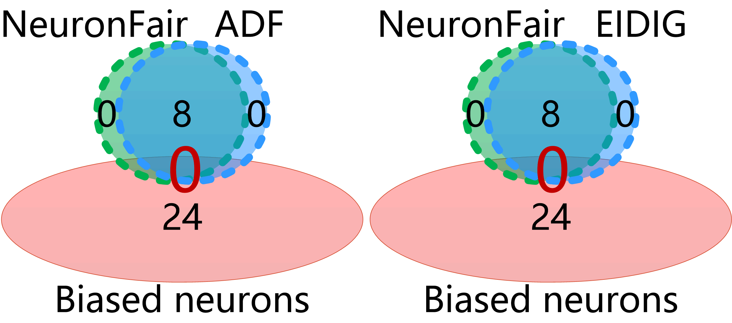
Biased neurons can be adopted to interpret the utility of IDIs and NeuronFair. First, IDIs trigger discrimination by activating biased neurons. For instance, the neurons activated by IDIs can cover most of the biased neurons in Fig. 6 (a), while the coverage of the biased neurons by non-IDIs of different methods is 0 in Fig. 6 (b). We can further interpret the utility of testing methods is related to the coverage of biased neurons, i.e., NeuronFair is more effective than ADF and EIDIG because they miss some discrimination contained in biased neurons while NeuronFair does not. For instance, in Fig. 6 (a), the NeuronFair’s IDIs activate all 24 biased neurons in the 2-nd layer of LFC-A classifier, while the neurons activated by other IDIs cannot cover all (15 for ADF and 18 for EIDIG).
Answer to RQ3: The main reason for NeuronFair’s utility is that its IDIs can activate more biased neurons. NeuronFair’s IDIs activate 100% biased neurons, while 62.5% for ADF and 75% for EIDIG.
5.4. Research Questions 4
How useful is the AUC metric for measuring DNNs’ fairness?
When answering this question, we refer to the following aspects: the consistency, significance, and complexity between AUC and DM-RS. The evaluation results on Adult and GerCre datasets with multiple sensitive attributes are shown in Tab. 9. From the results, we have the following observations.
-
•
In all cases, AUC can correctly distinguish DNNs’ fairness violations, i.e., AUC can serve the discrimination measurement of DNN. For instance, in Tab. 9, all of the values are 1.00, indicating that the discrimination ranking results of different DNNs based on AUC are completely consistent with those based on DM-RS. Since DNN’s decision results are determined by the neurons’ activation, we speculate that the biased decisions are also caused by the neurons’ activation, i.e., neurons contain discrimination information. Therefore, we can leverage the discrimination information in neurons to determine DNNs’ fairness.
-
•
In all cases, AUC can distinguish the different DNN’s discrimination more significantly than DM-RS, which is beneficial for a more accurate evaluation of IDIs of different testing methods. For instance, in Tab. 9, all values of AUC are higher than those of DM-RS, and the average value of AUC is 8.46 times that of DM-RS. The outstanding performance of AUC is mainly because we use the neurons’ ActDiff to measure the discrimination, which extracts more bias-related information from the whole DNN; while MD-RS only uses the bias-related information from the output layer.
-
•
The computational complexity of AUC is much lower than that of MD-RS, which is beneficial to quickly distinguish DNNs’ discrimination or the IDIs’ effect. The time frequency of AUC is based on Algorithm 1. Thus the time complexity of AUC is , while that of DM-RS is , where is the instance number, is the layer number, . It is mainly because AUC only conducts matrix operations, while DM-RS requires iterative operations until convergence.
Answer to RQ4: The AUC is useful for discrimination measurement. Compared to the results in Tab. 9, AUC is (1) 100% consistent with DM-RS, (2) 8.46 more significant than DM-RS, (3) low computational complexity with .
| Datasets | Sen. Att. | Metrics | Before | After | ||||||
|---|---|---|---|---|---|---|---|---|---|---|
|
|
ADF | EIDIG |
|
||||||
| Adult | gender | DM-RS | 2.88% | 0.45% | 0.44% | 0.26% | 0.21% | 0.19% | 1.00 | 0.0106 |
| AUC | 0.7513 | 0.1492 | 0.1482 | 0.1331 | 0.1098 | 0.0897 | 0.2563 | |||
| race | DM-RS | 8.91% | 0.61% | 0.81% | 0.75% | 0.69% | 0.57% | 1.00 | 0.0336 | |
| AUC | 0.8045 | 0.1466 | 0.1795 | 0.1652 | 0.1599 | 0.1070 | 0.2677 | |||
| age | DM-RS | 14.56% | 4.40% | 4.38% | 4.18% | 3.74% | 3.30% | 1.00 | 0.0433 | |
| AUC | 0.8591 | 0.1565 | 0.1520 | 0.1482 | 0.1347 | 0.1082 | 0.2941 | |||
| GerCre | gender | DM-RS | 5.16% | 0.76% | 0.67% | 0.55% | 0.56% | 0.49% | 1.00 | 0.0186 |
| AUC | 0.6308 | 0.1733 | 0.1568 | 0.1422 | 0.1524 | 0.0960 | 0.2004 | |||
| age | DM-RS | 30.90% | 3.66% | 3.46% | 3.31% | 3.21% | 2.32% | 1.00 | 0.1132 | |
| AUC | 0.8608 | 0.2046 | 0.1691 | 0.1568 | 0.1432 | 0.1204 | 0.2879 | |||
5.5. Research Questions 5
How generic is NeuronFair for the task of image IDI generation?
| Datasets | Sen. Att. | ADF | EIDIG | NeuronFair | |||
|---|---|---|---|---|---|---|---|
| #IDIs | GSR | #IDIs | GSR | #IDIs | GSR | ||
| ClbA-IN | gender | 1,087 | 11.58% | 2,895 | 12.50% | 10,578 | 69.90% |
| race | 11,908 | 33.54% | 25,180 | 59.87% | 51,529 | 90.15% | |
| LFW-IN | gender | 1,204 | 33.20% | 1,105 | 40.10% | 3,950 | 61.40% |
| race | 2,269 | 31.70% | 5,304 | 62.40% | 5,457 | 64.17% | |
| Datasets | Sen. Att. | Before | After | ||||||
| ADF | EIDIG | NeuronFair | |||||||
| AUC | DR | AUC | DR | AUC | DR | AUC | DR | ||
| ClbA-IN | gender | 0.3587 | 99.83% | 0.3328 | 97.20% | 0.3091 | 95.40% | 0.1650 | 98.40% |
| race | 0.4438 | 0.4045 | 96.50% | 0.3720 | 95.50% | 0.2501 | 98.90% | ||
| LFW-IN | gender | 0.3910 | 99.56% | 0.3524 | 95.30% | 0.3678 | 92.30% | 0.1091 | 98.90% |
| race | 0.4251 | 0.3984 | 98.10% | 0.3933 | 96.40% | 0.2240 | 99.10% | ||
When reporting the results, we focus on two aspects: generation quantity and quality.
Implementation details for NeuronFair generalized on image data: (1) we only perform comparisons with ADF and EIDIG at global phase, because the effect of ADF and EIDIG on DNNs is much better than that of Aequitas and SymbGen; (2) we remove the operation, set =0.15 for image, and all face images are used as input; (3) we retrain the face detector with all image IDIs of each method and measure its fairness improvement by AUC, (4) we measure the bias perturbation and sensitive attribute perturbation by -norm.
Generation Quantity. The evaluation results are shown in Tab. 10 measured by the IDIs number in global phase. From the results, we have the following observation.
-
•
In all cases, NeuronFair can obtain more IDIs than ADF and EIDIG, especially for the discrimination against race attribute. For instance, in Tab. 10, on average, NeuronFair generates 4.34 times and 2.07 times IDIs of ADF and EIDIG, respectively. The outstanding performance of NeuronFair is because it adopts dynamic loss to expand the valid input space while ADF and EIDIG do not consider the dynamics of search. Meanwhile, the number of IDIs generated by NeuronFair for race is 3.91 times that for gender. We speculate the reason is that the pixel information related to race is mainly skin color (i.e., light & dark, or black & white), while the pixel information related to gender is more diverse (such as hair, makeup, face shape, etc.). Therefore, the image IDIs generation for race is easier through manipulating skin color.
Generation Quality. The evaluation results are shown in Tabs. 10 and 11, including three scenarios: the generation success rate (GSR), the fairness improvement (AUC), and the detection rate (DR).
-
•
Among image data, image IDIs of NeuronFair are of higher quality than those of ADF and EIDIG, which can be applied to retrain face detectors and contribute to their fairness improvement in face detection scenarios. For instance, in Tab 10, on average, the GSR value of NeuronFair is 2.60 times and 1.63 times that of ADF and EIDIG, respectively. It is because NeuronFair reduces the probability of gradient vanishing, which in turn improves the probability of non-duplicate IDIs generation guided by the gradient. Hence, all GSR values of NeuronFair are higher than those of baselines. Meanwhile, the valid input space of NeuronFair is 1.67 times and 1.27 times that of ADF and EIDIG, respectively. Since the probability of falling into a local optimum is reduced by dynamically combining biased neurons, we can perform valid searches in limited instance space.
-
•
NeuronFair contributes more to the fairness improvement of the face detector, i.e., its generalization on image data is better than that of ADF and EIDIG. For instance, in Tab. 11, on average, the discrimination of detectors retrained with IDIs of NeuronFair dropped by 53.77%, while the AUC values of ADF and EIDIG only dropped by 8.06% and 10.90%, respectively. We speculate that the valid input space of NeuronFair is larger, so its IDIs can find potential discrimination that other methods’ IDIs cannot. Then improve the detector’s fairness through retraining.
-
•
NeuronFair hardly affects the detector’s DR values while improving its fairness. For instance, in Tab. 11, on average, the DR value of detectors retrained with NeuronFair’s IDIs only dropped by 0.87%, while that of ADF and EIDIG dropped by 2.92% and 4.80%, respectively. We compare the norm of and generated by different methods, and find that of NeuronFair is much lower than that of ADF and EIDIG. Therefore, NeuronFair can not only improve the detector’s fairness but also maintain its detection performance.
Answer to RQ5: The generalization performance of NeuronFair on the image dataset is better than the SOTA methods (i.e., ADF and EIDIG) in two aspects: (1) quantity - it generates 4.34 and 2.07 image IDIs on average compared to ADF and EIDIG, respectively; (2) quality - it searches 1.47 input space with more than 2.11 GSR on average, it is beneficial to detectors’ fairness improvement of 53.77% on average but hardly affects their detection performance. Thus, NeuronFair shows better generalization performance than ADF and EIDIG.
6. Threats to Validity
Correlation between attributes. The attributes of unstructured data are not as clear as structured data, so we provide a generalization framework that can modify sensitive attributes. However, there is a correlation between attributes, i.e., after the perturbation for one sensitive attribute is added, another attribute may also be changed. Since the transferability of perturbation is not robust. the slight attribute change will not affect our IDI generation.
Sensitive attributes. We consider only one sensitive attribute at a time for our experiments. However, considering multiple protected attributes will not hamper the effectiveness or generalization offered by our novel testing technique, but will certainly lead to an increase in execution time. This increase is attributed towards the fact that the algorithm in such a case, needs to consider all the possible combinations of their unique values.
Access to DNNs. NeuronFair is white-box testing that generates IDIs based on the biased neurons inside DNNs, which means it requires accessing to DNNs. It is widely accepted that DNN testing could have full knowledge of the target model in software engineering.
7. Related Works
Fairness Testing. Based on the software engineering point of view, several works on testing the fairness of traditional ML models are proposed (Tramèr et al., 2017; Adebayo and Kagal, 2016; Udeshi et al., 2018; Galhotra et al., 2017; Aggarwal et al., 2018; Zhang and Harman, 2021). To uncover their fairness violations, Galhotra et al. (Galhotra et al., 2017) firstly proposed Themis, a fairness testing method for software, which measures the discrimination in software through counting the frequency of IDIs in the input space. However, its efficiency for IDIs generation is unsatisfactory. To improve the generation speed of Themis, Udeshi et al. (Udeshi et al., 2018) proposed a faster generation algorithm, Aequitas, which uncovers fairness violations by probabilistic search over the input space. Aequitas adopts a two-phase operation in which the IDIs generated globally are used as seeds for the local generation. However, Aequitas uses a global sampling distribution for all the inputs, which leads to the limitation that it can only search in narrow input space and easily falls into the local optimum. Thus, Aequitas’s IDIs lack diversity. To further improve the instance diversity, Agarwal et al. (Aggarwal et al., 2018) designed a new testing method, SymbGen, which combines the symbolic execution along with the local interpretation for the generation of effective instances. SymbGen constructs the local explainer of the complex model at first and then searches for IDIs based on the fitted decision boundary. Therefore, its instance effectiveness almost depends on the performance of the explainer.
The above-mentioned methods mainly deal with traditional ML models, which cannot directly be applied to deal with DNNs. Recently, several methods have been proposed specifically for DNNs. For instance, Zhang et al. (Zhang et al., 2020) first proposed a fairness testing method specifically for DNNs, ADF, which guides the search direction through gradients. The authors proved that its effectiveness and efficiency of IDIs generation for DNNs are greatly improved based on the guidance of gradients. Based on the ADF (Zhang et al., 2020), Zhang et al. (Zhang et al., 2021) designed a framework EIDIG for discovering individual fairness violations, which adopts prior information to accelerate the convergence of iterative optimization. However, there is still a problem of gradient vanishing, which may lead to local optimization.
Neuron-based DNN Interpretation. Kim et al. (Kim et al., 2018) first introduced concept activation vectors, which provide an interpretation of a DNN’s internal state (i.e., the activation output in the hidden layer). They viewed the high-dimensional internal state of a DNN as an aid, and interpreted which concept is important to the classification result. Inspired by the concept activation vectors, Du et al. (Du et al., 2019) suggested that interpretability can serve as a useful ingredient to diagnose the reasons that lead to algorithmic discrimination. The above methods study the activation output of one hidden layer, while Liu et al. (Liu et al., 2019) studied the activation state of a single neuron. They observed that the neuron activation is related to the DNNs’ robustness, and used the abnormal activation of a single neuron to detect backdoor attacks. These methods leverage the internal state to interpret DNNs’ classification performance and robustness, which inspires us to use it to interpret DNNs’ biased decision.
8. Conclusions
We propose an interpretable white-box fairness testing method, NeuronFair, to efficiently generate IDIs for DNNs based on biased neurons. Our method provides discrimination interpretation and IDI generation for different data forms. In the discrimination interpretation, AS curve and AUC measurement are designed to qualitatively and quantitatively interpret the severity of discrimination in each layer of DNNs, respectively. In the IDI generation, a global phase and a local phase collaborate to systematically search the input space for IDIs with the guidance of momentum acceleration and dynamic loss. Further, NeuronFair can process not only structured data but also unstructured data, e.g., image, text, etc. We compare NeuronFair with four SOTA methods in 5 structured datasets and 2 face image datasets against 7 DNNs, the results show that NeuronFair has significantly better performance in terms of interpretability, generation effectiveness, and data generalization.
Acknowledgment
This research was supported by the National Natural Science Foundation of China (Nos. 62072406, 62102359), the Key R&D Projects in Zhejiang Province (Nos. 2021C01117 and 2022C01018), the “Ten Thousand Talents Program” in Zhejiang Province (2020R52011).
References
- (1)
- Adebayo and Kagal (2016) Julius Adebayo and Lalana Kagal. 2016. Iterative Orthogonal Feature Projection for Diagnosing Bias in Black-Box Models. CoRR abs/1611.04967 (2016), 1–5. arXiv:1611.04967 http://arxiv.org/abs/1611.04967
- Aggarwal et al. (2018) Aniya Aggarwal, Pranay Lohia, Seema Nagar, Kuntal Dey, and Diptikalyan Saha. 2018. Automated Test Generation to Detect Individual Discrimination in AI Models. CoRR abs/1809.03260 (2018), 1–8. arXiv:1809.03260 http://arxiv.org/abs/1809.03260
- Aggarwal et al. (2019) Aniya Aggarwal, Pranay Lohia, Seema Nagar, Kuntal Dey, and Diptikalyan Saha. 2019. Black box fairness testing of machine learning models. In Proceedings of the ACM Joint Meeting on European Software Engineering Conference and Symposium on the Foundations of Software Engineering, ESEC/SIGSOFT FSE 2019, Tallinn, Estonia, August 26-30, 2019. ACM, New York, NY, 625–635. https://doi.org/10.1145/3338906.3338937
- Amini et al. (2019) Alexander Amini, Ava P. Soleimany, Wilko Schwarting, Sangeeta N. Bhatia, and Daniela Rus. 2019. Uncovering and Mitigating Algorithmic Bias through Learned Latent Structure. In Proceedings of the 2019 AAAI/ACM Conference on AI, Ethics, and Society, AIES 2019, Honolulu, HI, USA, January 27-28, 2019. ACM, New York, NY, 289–295. https://doi.org/10.1145/3306618.3314243
- Badar et al. (2020) Maryam Badar, Muhammad Haris, and Anam Fatima. 2020. Application of deep learning for retinal image analysis: A review. Computer Science Review 35 (2020), 1–18. http://dx.doi.org/10.1016/j.cosrev.2019.100203
- Bellamy et al. (2018) Rachel K. E. Bellamy, Kuntal Dey, Michael Hind, Samuel C. Hoffman, Stephanie Houde, Kalapriya Kannan, Pranay Lohia, Jacquelyn Martino, Sameep Mehta, Aleksandra Mojsilovic, Seema Nagar, Karthikeyan Natesan Ramamurthy, John Richards, Diptikalyan Saha, Prasanna Sattigeri, Moninder Singh, Kush R. Varshney, and Yunfeng Zhang. 2018. AI Fairness 360: An Extensible Toolkit for Detecting, Understanding, and Mitigating Unwanted Algorithmic Bias. https://arxiv.org/abs/1810.01943
- Biswas and Rajan (2020) Sumon Biswas and Hridesh Rajan. 2020. Do the machine learning models on a crowd sourced platform exhibit bias? an empirical study on model fairness. In ESEC/FSE ’20: 28th ACM Joint European Software Engineering Conference and Symposium on the Foundations of Software Engineering, Virtual Event, USA, November 8-13, 2020, Prem Devanbu, Myra B. Cohen, and Thomas Zimmermann (Eds.). ACM, New York, NY, 642–653. https://doi.org/10.1145/3368089.3409704
- Biswas and Rajan (2021) Sumon Biswas and Hridesh Rajan. 2021. Fair preprocessing: towards understanding compositional fairness of data transformers in machine learning pipeline. In ESEC/FSE ’21: 29th ACM Joint European Software Engineering Conference and Symposium on the Foundations of Software Engineering, Athens, Greece, August 23-28, 2021, Diomidis Spinellis, Georgios Gousios, Marsha Chechik, and Massimiliano Di Penta (Eds.). ACM, New York, NY, 981–993. https://doi.org/10.1145/3468264.3468536
- Black et al. (2020) Emily Black, Samuel Yeom, and Matt Fredrikson. 2020. FlipTest: fairness testing via optimal transport. In FAT* ’20: Conference on Fairness, Accountability, and Transparency, Barcelona, Spain, January 27-30, 2020. ACM, New York, NY, 111–121. https://doi.org/10.1145/3351095.3372845
- Brendel et al. (2018) Wieland Brendel, Jonas Rauber, and Matthias Bethge. 2018. Decision-based adversarial attacks: Reliable attacks against black-box machine learning models. In 6th International Conference on Learning Representations, ICLR 2018, Vancouver, BC, Canada, April 30-May 3, 2018. OpenReview.net, [C/OL, 2018-2-16], 1–12. https://openreview.net/forum?id=SyZI0GWCZ
- Brun and Meliou (2018) Yuriy Brun and Alexandra Meliou. 2018. Software fairness. In Proceedings of the 2018 ACM Joint Meeting on European Software Engineering Conference and Symposium on the Foundations of Software Engineering, ESEC/SIGSOFT FSE 2018, Lake Buena Vista, FL, USA, November 04-09, 2018, Gary T. Leavens, Alessandro Garcia, and Corina S. Pasareanu (Eds.). ACM, New York, NY, 754–759. https://doi.org/10.1145/3236024.3264838
- Buolamwini and Gebru (2018) Joy Buolamwini and Timnit Gebru. 2018. Gender Shades: Intersectional Accuracy Disparities in Commercial Gender Classification. In Conference on Fairness, Accountability and Transparency, FAT 2018, 23-24 February 2018, New York, NY, USA (Proceedings of Machine Learning Research, Vol. 81). PMLR, Stockholm, Sweden, 77–91. http://proceedings.mlr.press/v81/buolamwini18a.html
- Chen et al. (2020a) Jinyin Chen, Keke Hu, Yue Yu, Zhuangzhi Chen, Qi Xuan, Yi Liu, and Vladimir Filkov. 2020a. Software visualization and deep transfer learning for effective software defect prediction. In ICSE ’20: 42nd International Conference on Software Engineering, Seoul, South Korea, 27 June - 19 July, 2020, Gregg Rothermel and Doo-Hwan Bae (Eds.). ACM, New York, NY, 578–589. https://doi.org/10.1145/3377811.3380389
- Chen et al. (2020b) Jinyin Chen, Haibin Zheng, Hui Xiong, Shijing Shen, and Mengmeng Su. 2020b. MAG-GAN: Massive Attack Generator via GAN. Information Sciences 536 (2020), 67–90. http://dx.doi.org/10.1016/j.ins.2020.04.019
- Chen et al. (2017) PinYu Chen, Huan Zhang, Yash Sharma, Jinfeng Yi, and ChoJui Hsieh. 2017. ZOO: Zeroth order optimization based black-box attacks to deep neural networks without training substitute models. In Proceedings of the 10th ACM Workshop on Artificial Intelligence and Security, AISec@CCS 2017, Dallas, TX, USA, November 3, 2017. ACM, New York, NY, 15–26. https://doi.org/10.1145/3128572.3140448
- Clegg et al. (2019) Benjamin S. Clegg, Siobhán North, Phil McMinn, and Gordon Fraser. 2019. Simulating student mistakes to evaluate the fairness of automated grading. In Proceedings of the 41st International Conference on Software Engineering: Software Engineering Education and Training, ICSE (SEET) 2019, Montreal, QC, Canada, May 25-31, 2019, Sarah Beecham and Daniela E. Damian (Eds.). IEEE / ACM, Piscataway, NJ, 121–125. https://doi.org/10.1109/ICSE-SEET.2019.00021
- Deng et al. (2009) Jia Deng, Wei Dong, Richard Socher, Li-Jia Li, Kai Li, and Li Fei-Fei. 2009. ImageNet: A Large-Scale Hierarchical Image Database. In 2009 IEEE Computer Society Conference on Computer Vision and Pattern Recognition (CVPR 2009), 20-25 June 2009, Miami, Florida, USA, Vol. 1-4. IEEE Computer Society, Computer Society Los Alamitos, CA, 248–255. https://doi.org/10.1109/CVPR.2009.5206848
- Devanbu et al. (2020) Prem Devanbu, Matthew Dwyer, Sebastian Elbaum, Michael Lowry, Kevin Moran, Denys Poshyvanyk, Baishakhi Ray, Rishabh Singh, and Xiangyu Zhang. 2020. Deep Learning & Software Engineering: State of Research and Future Directions. arXiv:2009.08525 [cs.SE]
- Devlin et al. (2019) Jacob Devlin, Ming-Wei Chang, Kenton Lee, and Kristina Toutanova. 2019. BERT: Pre-training of deep bidirectional transformers for language understanding. In Proceedings of the 2019 Conference of the North American Chapter of the Association for Computational Linguistics: Human Language Technologies, NAACL-HLT 2019, Minneapolis, MN, USA, June 2-7, 2019. Association for Computational Linguistics, Stroudsburg,PA, 4171–4186. https://doi.org/10.18653/v1/n19-1423
- Dong et al. (2018) Yinpeng Dong, Fangzhou Liao, Tianyu Pang, Hang Su, Jun Zhu, Xiaolin Hu, and Jianguo Li. 2018. Boosting Adversarial Attacks with Momentum. In 2018 IEEE Conference on Computer Vision and Pattern Recognition, CVPR 2018, Salt Lake City, UT, USA, June 18-22, 2018. IEEE Computer Society, Computer Society Los Alamitos, CA, 9185–9193. https://doi.org/10.1109/CVPR.2018.00957
- Du et al. (2019) Mengnan Du, Fan Yang, Na Zou, and Xia Hu. 2019. Fairness in Deep Learning: A Computational Perspective. CoRR abs/1908.08843 (2019), 1–9. arXiv:1908.08843 http://arxiv.org/abs/1908.08843
- Dwork et al. (2012) Cynthia Dwork, Moritz Hardt, Toniann Pitassi, Omer Reingold, and Richard S. Zemel. 2012. Fairness through awareness. In Innovations in Theoretical Computer Science 2012, Cambridge, MA, USA, January 8-10, 2012. ACM, New York, NY, 214–226. https://doi.org/10.1145/2090236.2090255
- Farahani et al. (2021) Ali Farahani, Liliana Pasquale, Amel Bennaceur, Thomas Welsh, and Bashar Nuseibeh. 2021. On Adaptive Fairness in Software Systems. In 16th International Symposium on Software Engineering for Adaptive and Self-Managing Systems, SEAMS@ICSE 2021, Madrid, Spain, May 18-24, 2021. IEEE, Piscataway, NJ, 97–103. https://doi.org/10.1109/SEAMS51251.2021.00022
- Galhotra et al. (2017) Sainyam Galhotra, Yuriy Brun, and Alexandra Meliou. 2017. Fairness testing: testing software for discrimination. In Proceedings of the 2017 11th Joint Meeting on Foundations of Software Engineering, ESEC/FSE 2017, Paderborn, Germany, September 4-8, 2017. ACM, New York, NY, 498–510. https://doi.org/10.1145/3106237.3106277
- Gaur et al. (2021) Bodhvi Gaur, Gurpreet Singh Saluja, Hamsa Bharathi Sivakumar, and Sanjay Singh. 2021. Semi-supervised deep learning based named entity recognition model to parse education section of resumes. Neural Computing and Applications 33 (2021), 5705–5718. https://doi.org/10.1007/s00521-020-05351-2
- Germán et al. (2018) Daniel M. Germán, Gregorio Robles, Germán Poo-Caamaño, Xin Yang, Hajimu Iida, and Katsuro Inoue. 2018. ”Was my contribution fairly reviewed?”: a framework to study the perception of fairness in modern code reviews. In Proceedings of the 40th International Conference on Software Engineering, ICSE 2018, Gothenburg, Sweden, May 27 - June 03, 2018, Michel Chaudron, Ivica Crnkovic, Marsha Chechik, and Mark Harman (Eds.). ACM, New York, NY, 523–534. https://doi.org/10.1145/3180155.3180217
- Goodfellow et al. (2015) Ian J. Goodfellow, Jonathon Shlens, and Christian Szegedy. 2015. Explaining and harnessing adversarial examples. In 3rd International Conference on Learning Representations, ICLR 2015, San Diego, CA, USA, May 7-9, 2015. Arxiv, [C/OL, 2015-5-20], 1–10. http://arxiv.org/abs/1412.6572
- He et al. (2016) Kaiming He, Xiangyu Zhang, Shaoqing Ren, and Jian Sun. 2016. Deep residual learning for image recognition. In 2016 IEEE Conference on Computer Vision and Pattern Recognition, CVPR 2016, Las Vegas, NV, USA, June 27-30, 2016. IEEE Computer Society, Computer Society Los Alamitos, CA, 770–778. https://doi.org/10.1109/CVPR.2016.90
- Holstein and Dodig-Crnkovic (2018) Tobias Holstein and Gordana Dodig-Crnkovic. 2018. Avoiding the intrinsic unfairness of the trolley problem. In Proceedings of the International Workshop on Software Fairness, FairWare@ICSE 2018, Gothenburg, Sweden, May 29, 2018, Yuriy Brun, Brittany Johnson, and Alexandra Meliou (Eds.). ACM, New York, NY, 32–37. https://doi.org/10.1145/3194770.3194772
- Huang et al. (2018) Chao Huang, Junbo Zhang, Yu Zheng, and Nitesh V. Chawla. 2018. DeepCrime: Attentive Hierarchical Recurrent Networks for Crime Prediction. In Proceedings of the 27th ACM International Conference on Information and Knowledge Management, CIKM 2018, Torino, Italy, October 22-26, 2018. ACM, New York, NY, 1423–1432. https://doi.org/10.1145/3269206.3271793
- Huang et al. (2008) Gary B. Huang, Marwan Mattar, Tamara Berg, and Eric Learned-Miller. 2008. Labeled Faces in the Wild: A Database forStudying Face Recognition in Unconstrained Environments. In Workshop on Faces in ’Real-Life’ Images: Detection, Alignment, and Recognition. Erik Learned-Miller and Andras Ferencz and Frédéric Jurie, HAL-inria, Marseille, France, 1–15. https://hal.inria.fr/inria-00321923
- Huang et al. (2021) Yujin Huang, Han Hu, and Chunyang Chen. 2021. Robustness of on-Device Models: Adversarial Attack to Deep Learning Models on Android Apps. In 43rd IEEE/ACM International Conference on Software Engineering: Software Engineering in Practice, ICSE (SEIP) 2021, Madrid, Spain, May 25-28, 2021. IEEE, Piscataway, NJ, 101–110. https://doi.org/10.1109/ICSE-SEIP52600.2021.00019
- Kim et al. (2018) Been Kim, Martin Wattenberg, Justin Gilmer, Carrie J. Cai, James Wexler, Fernanda B. Viégas, and Rory Sayres. 2018. Interpretability Beyond Feature Attribution: Quantitative Testing with Concept Activation Vectors (TCAV). In Proceedings of the 35th International Conference on Machine Learning, ICML 2018, Stockholmsmässan, Stockholm, Sweden, July 10-15, 2018 (Proceedings of Machine Learning Research, Vol. 80). PMLR, Stockholm, Sweden, 2673–2682. http://proceedings.mlr.press/v80/kim18d.html
- Klare et al. (2012) Brendan Klare, Mark James Burge, Joshua C. Klontz, Richard W. Vorder Bruegge, and Anil K. Jain. 2012. Face Recognition Performance: Role of Demographic Information. IEEE Trans. Inf. Forensics Secur. 7, 6 (2012), 1789–1801. https://doi.org/10.1109/TIFS.2012.2214212
- Kohavi (1996) Ron Kohavi. 1996. Scaling Up the Accuracy of Naive-Bayes Classifiers: A Decision-Tree Hybrid. In Proceedings of the Second International Conference on Knowledge Discovery and Data Mining (KDD-96), Portland, Oregon, USA. AAAI Press, Menlo Park, CA, 202–207. http://www.aaai.org/Library/KDD/1996/kdd96-033.php
- Kurakin et al. (2017) Alexey Kurakin, Ian J. Goodfellow, and Samy Bengio. 2017. Adversarial examples in the physical world. In 5th International Conference on Learning Representations, ICLR 2017, Toulon, France, April 24-26, 2017, Workshop Track Proceedings. OpenReview.net, [C/OL, 2017-2-11], 1–14. https://openreview.net/forum?id=HJGU3Rodl
- Kusner et al. (2017) Matt J. Kusner, Joshua R. Loftus, Chris Russell, and Ricardo Silva. 2017. Counterfactual Fairness. In Advances in Neural Information Processing Systems 30: Annual Conference on Neural Information Processing Systems 2017, December 4-9, 2017, Long Beach, CA, USA, Isabelle Guyon, Ulrike von Luxburg, Samy Bengio, Hanna M. Wallach, Rob Fergus, S. V. N. Vishwanathan, and Roman Garnett (Eds.). NEURAL INFORMATION PROCESSING SYSTEMS, La Jolla, California, 4066–4076. https://proceedings.neurips.cc/paper/2017/hash/a486cd07e4ac3d270571622f4f316ec5-Abstract.html
- LeCun et al. (2015) Yann LeCun, Yoshua Bengio, and Geoffrey Hinton. 2015. Deep learning. NATURE 521, 7553 (2015), 436–444. https://doi.org/10.1038/nature14539
- Li et al. (2021) Yuanchun Li, Jiayi Hua, Haoyu Wang, Chunyang Chen, and Yunxin Liu. 2021. DeepPayload: Black-box Backdoor Attack on Deep Learning Models through Neural Payload Injection. In 43rd IEEE/ACM International Conference on Software Engineering, ICSE 2021, Madrid, Spain, 22-30 May 2021. IEEE, Piscataway, NJ, 263–274. https://doi.org/10.1109/ICSE43902.2021.00035
- Liu et al. (2019) Yingqi Liu, Wen-Chuan Lee, Guanhong Tao, Shiqing Ma, Yousra Aafer, and Xiangyu Zhang. 2019. ABS: Scanning Neural Networks for Back-doors by Artificial Brain Stimulation. In Proceedings of the 2019 ACM SIGSAC Conference on Computer and Communications Security, CCS 2019, London, UK, November 11-15, 2019. ACM, New York, NY, 1265–1282. https://doi.org/10.1145/3319535.3363216
- Liu et al. (2015) Ziwei Liu, Ping Luo, Xiaogang Wang, and Xiaoou Tang. 2015. Deep Learning Face Attributes in the Wild. In 2015 IEEE International Conference on Computer Vision, ICCV 2015, Santiago, Chile, December 7-13, 2015. IEEE Computer Society, Computer Society Los Alamitos, CA, 3730–3738. https://doi.org/10.1109/ICCV.2015.425
- Mai et al. (2019) Feng Mai, Shaonan Tian, Chihoon Lee, and Ling Ma. 2019. Deep learning models for bankruptcy prediction using textual disclosures. Eur. J. Oper. Res. 274, 2 (2019), 743–758. https://doi.org/10.1016/j.ejor.2018.10.024
- Melton (2018) Hayden Melton. 2018. On fairness in continuous electronic markets. In Proceedings of the International Workshop on Software Fairness, FairWare@ICSE 2018, Gothenburg, Sweden, May 29, 2018, Yuriy Brun, Brittany Johnson, and Alexandra Meliou (Eds.). ACM, New York, NY, 29–31. https://doi.org/10.1145/3194770.3194771
- Meng et al. (2021) Linghan Meng, Yanhui Li, Lin Chen, Zhi Wang, Di Wu, Yuming Zhou, and Baowen Xu. 2021. Measuring Discrimination to Boost Comparative Testing for Multiple Deep Learning Models. In 43rd IEEE/ACM International Conference on Software Engineering, ICSE 2021, Madrid, Spain, 22-30 May 2021. IEEE, Piscataway, NJ, 385–396. https://doi.org/10.1109/ICSE43902.2021.00045
- Mirabella et al. (2021) A. Giuliano Mirabella, Alberto Martin-Lopez, Sergio Segura, Luis Valencia-Cabrera, and Antonio Ruiz-Cortés. 2021. Deep Learning-Based Prediction of Test Input Validity for RESTful APIs. In 3rd IEEE/ACM International Workshop on Deep Learning for Testing and Testing for Deep Learning, DeepTest@ICSE 2021, Madrid, Spain, June 1, 2021. IEEE, Piscataway, NJ, 9–16. https://doi.org/10.1109/DeepTest52559.2021.00008
- Pei et al. (2019) Kexin Pei, Yinzhi Cao, Junfeng Yang, and Suman Jana. 2019. DeepXplore: automated whitebox testing of deep learning systems. Commun. ACM 62, 11 (2019), 137–145. https://doi.org/10.1145/3361566
- Ramadan et al. (2018) Qusai Ramadan, Amir Shayan Ahmadian, Daniel Strüber, Jan Jürjens, and Steffen Staab. 2018. Model-based discrimination analysis: a position paper. In Proceedings of the International Workshop on Software Fairness, FairWare@ICSE 2018, Gothenburg, Sweden, May 29, 2018, Yuriy Brun, Brittany Johnson, and Alexandra Meliou (Eds.). ACM, New York, NY, 22–28. https://doi.org/10.1145/3194770.3194775
- Sedaghatbaf et al. (2021) Ali Sedaghatbaf, Mahshid Helali Moghadam, and Mehrdad Saadatmand. 2021. Automated Performance Testing Based on Active Deep Learning. In 2nd IEEE/ACM International Conference on Automation of Software Test, AST@ICSE 2021, Madrid, Spain, May 20-21, 2021. IEEE, Piscataway, NJ, 11–19. https://doi.org/10.1109/AST52587.2021.00010
- Simonyan and Zisserman (2015) Karen Simonyan and Andrew Zisserman. 2015. Very deep convolutional networks for large-scale image recognition. In 3rd International Conference on Learning Representations, ICLR 2015, San Diego, CA, USA, May 7-9, 2015. Arxiv, [C/OL, 2015-4-10], 1–14. http://arxiv.org/abs/1409.1556
- Tabacof and Valle (2016) Pedro Tabacof and Eduardo Valle. 2016. Exploring the space of adversarial images. In 2016 International Joint Conference on Neural Networks, IJCNN 2016, Vancouver, BC, Canada, July 24-29, 2016, Vol. 2016-October. IEEE, Piscataway, NJ, 426–433. https://doi.org/10.1109/IJCNN.2016.7727230
- Tramèr et al. (2017) Florian Tramèr, Vaggelis Atlidakis, Roxana Geambasu, Daniel J. Hsu, Jean-Pierre Hubaux, Mathias Humbert, Ari Juels, and Huang Lin. 2017. FairTest: Discovering Unwarranted Associations in Data-Driven Applications. In 2017 IEEE European Symposium on Security and Privacy, EuroS&P 2017, Paris, France, April 26-28, 2017. IEEE, Piscataway, NJ, 401–416. https://doi.org/10.1109/EuroSP.2017.29
- Udeshi et al. (2018) Sakshi Udeshi, Pryanshu Arora, and Sudipta Chattopadhyay. 2018. Automated directed fairness testing. In Proceedings of the 33rd ACM/IEEE International Conference on Automated Software Engineering, ASE 2018, Montpellier, France, September 3-7, 2018. ACM, New York, NY, 98–108. https://doi.org/10.1145/3238147.3238165
- Verma and Rubin (2018) Sahil Verma and Julia Rubin. 2018. Fairness definitions explained. In Proceedings of the International Workshop on Software Fairness, FairWare@ICSE 2018, Gothenburg, Sweden, May 29, 2018. ACM, New York, NY, 1–7. https://doi.org/10.1145/3194770.3194776
- Wang et al. (2020) Zeyu Wang, Klint Qinami, Ioannis Christos Karakozis, Kyle Genova, Prem Nair, Kenji Hata, and Olga Russakovsky. 2020. Towards Fairness in Visual Recognition: Effective Strategies for Bias Mitigation. In 2020 IEEE/CVF Conference on Computer Vision and Pattern Recognition, CVPR 2020, Seattle, WA, USA, June 13-19, 2020. IEEE, Piscataway, NJ, 8916–8925. https://doi.org/10.1109/CVPR42600.2020.00894
- Zhang and Harman (2021) Jie M. Zhang and Mark Harman. 2021. ”Ignorance and Prejudice” in Software Fairness. In 43rd IEEE/ACM International Conference on Software Engineering, ICSE 2021, Madrid, Spain, 22-30 May 2021. IEEE, Piscataway, NJ, 1436–1447. https://doi.org/10.1109/ICSE43902.2021.00129
- Zhang et al. (2021) Lingfeng Zhang, Yueling Zhang, and Min Zhang. 2021. Efficient white-box fairness testing through gradient search. In ISSTA ’21: 30th ACM SIGSOFT International Symposium on Software Testing and Analysis, Virtual Event, Denmark, July 11-17, 2021, Cristian Cadar and Xiangyu Zhang (Eds.). ACM, New York, NY, 103–114. https://doi.org/10.1145/3460319.3464820
- Zhang et al. (2020) Peixin Zhang, Jingyi Wang, Jun Sun, Guoliang Dong, Xinyu Wang, Xingen Wang, Jin Song Dong, and Ting Dai. 2020. White-box fairness testing through adversarial sampling. In ICSE ’20: 42nd International Conference on Software Engineering, Seoul, South Korea, 27 June - 19 July, 2020. ACM, New York, NY, 949–960. https://doi.org/10.1145/3377811.3380331