Neural KEM: A Kernel Method with Deep Coefficient Prior for PET Image Reconstruction

PET projection measurement $\bm{y}=\left\{y_{i}\right\}_{i=1}^{N}$ can be well modeled as independent Poisson random variables using the log-likelihood function [1],

$$L(\bm{y}|\bm{x})=\sum_{i=1}^{N}y_{i}\log\overline{y}_{i}-\overline{y}_{i}-\log y_{i}!,$$

(1)

where the expectation of the projection data, $\overline{\bm{y}}=\left\{\overline{y}_{i}\right\}_{i=1}^{N}$, is related to the unknown activity image $\bm{x}=\left\{x_{j}\right\}_{j=1}^{J}$ through

$$\overline{\bm{y}}=\bm{P}\bm{x}+\bm{r},$$

(2)

where $x_{j}$ denotes the PET image intensity value in pixel $j$. $N$ is the total number of detector pairs and $J$ is the number of image pixels. $\bm{P}$ is the detection probability matrix and includes normalization factors for scanner sensitivity, scan duration, deadtime correction and attenuation correction. $\bm{r}$ is the expectation of random and scattered events[1].

The maximum likelihood estimate of the activity image $\bm{x}$ is found by maximizing the Poisson log-likelihood,

$$\hat{\bm{x}}=\arg\max\limits_{\bm{x}\geq 0}L(\bm{y}|\bm{x}).$$

(3)

A common way of seeking the solution of (3) is the maximum likelihood expectation maximization (ML-EM) algorithm [37].

The image estimate by standard MLEM is commonly noisy due to the limited counting statistics of PET emission data. To suppress noise, the kernel method[2] incorporates an image prior into the forward projection of PET reconstruction by describing the image intensity $x_{j}$ using kernels,

$$x_{j}=\sum_{l\in\mathcal{N}_{j}}\bm{\alpha}_{l}\kappa(\bm{f}_{j},\bm{f}_{l}),$$

(4)

where $\mathcal{N}_{j}$ defines the neighborhood of pixel $j$, e.g., by the k-nearest neighbors (kNN, [38]). $\kappa(\cdot,\cdot)$ is the kernel function (e.g., radial Gaussian) and $\bm{f}$ denotes the low-dimensional feature vector that is extracted at each pixel from the image prior $\bm{z}$ (e.g. the composite images in dynamic PET or anatomical image in PET/MR or PET/CT). The equivalent matrix-vector form of (4) is

$$\bm{x}=\bm{K}\bm{\alpha},$$

(5)

where $\bm{K}$ is a sparse square kernel matrix with its ($j,l$)th element being $\kappa(\bm{f}_{j},\bm{f}_{l})$. $\bm{\alpha}$ denotes the corresponding kernel coefficient image.

Substituting the kernelized image model (5) into the standard PET forward projection model in (2) gives the following kernelized forward projection model for PET image reconstruction,

$$\overline{\bm{y}}=\bm{P}\bm{K}\bm{\alpha}+\bm{r}.$$

(6)

The maximium-likelihood estimate of $\bm{\alpha}$ can be found by the kernel EM algorithm [2],

$$\bm{\alpha}^{n+1}=\frac{\bm{\alpha}^{n}}{\bm{w}}\cdot\left(\bm{K}^{T}\bm{P}^{T}\frac{\bm{y}}{\bm{P}\bm{K}\bm{\alpha}^{n}+\bm{r}}\right),$$

(7)

where

$$\bm{w}=\bm{K}^{T}\bm{P}^{T}\bm{1}_{N},$$

(8)

and $\bm{1}_{N}$ is a vector with all elements being 1. $n$ denotes the iteration number and the superscript “$T$” denotes matrix transpose. The vector multiplication and division are element-wise operations. Note that the KEM update becomes the standard EM update if $\bm{K}$ is an identity matrix. Once $\bm{\alpha}$ is estimated, the final reconstructed PET image is given by

$$\hat{\bm{x}}=\bm{K}\hat{\bm{\alpha}}.$$

(9)

Note that the same update equation (7) is also used by the sieves method [11]. The difference is that the sieves method uses a stationary Gaussian kernel [11], while the kernel method here uses data-driven spatially variant kernels that are derived from the image prior $\bm{z}$.

The estimated kernel coefficient image $\bm{\alpha}$ by the standard kernel method [2] may still suffer from noise, as demonstrated later in this paper. One possible way for improvement is to add an explicit penalty function to stabilize the estimation of $\bm{\alpha}$ as indicated in the original kernel method [2], which however may result in a more challenging optimization problem and involves at least one more regularization parameter to tune.

The DIP method for PET reconstruction is proposed in [18] based on the representation ability of CNNs. Instead of using the linear kernel representation in (6), the PET image $\bm{x}$ can be also described by a nonlinear representation using neural networks and the image prior data $\bm{z}$,

$$\bm{x}=\bm{\beta}(\bm{\theta}|\bm{z}),$$

(10)

where $\bm{\beta}$ is a neural netwok model with $\bm{z}$ the input images and $\bm{\theta}$ the network weights. After substituting the DIP model (10) into (2), the PET forward projection model becomes

$$\overline{\bm{y}}=\bm{P}\bm{\beta}(\bm{\theta}|\bm{z})+\bm{r}.$$

(11)

The maximum-likelihood estimate of the unknown $\bm{\theta}$ is obtained by

$$\hat{\bm{\theta}}=\arg\max\limits_{\bm{\theta}}L\Big{(}\bm{y}|\bm{\beta}(\bm{\theta}|\bm{z})\Big{)}.$$

(12)

Once $\bm{\theta}$ is estimated, the PET activity image is calculated as

$$\hat{\bm{x}}=\bm{\beta}(\hat{\bm{\theta}}|\bm{z}).$$

(13)

To solve the resulting nonlinear optimization problem, Gong et al. [18] use the ADMM algorithm,

$$\bm{x}^{n+1}=\arg\max\limits_{\bm{x}}L(\bm{y}|\bm{x})-\frac{\rho}{2}||\bm{x}-\bm{\beta}(\bm{\theta}^{n}|\bm{z})+\bm{\mu}||^{2},$$

(14)

$$\bm{\theta}^{n+1}=\arg\min\limits_{\bm{\theta}}||\bm{\beta}(\bm{\theta}|\bm{z})-(\bm{x}^{n+1}+\bm{\mu}^{n})||^{2},$$

(15)

$$\bm{\mu}^{n+1}=\bm{\mu}^{n}+\bm{x}^{n+1}-\bm{\beta}(\bm{\theta}^{n+1}|\bm{z}),$$

(16)

where the subproblem (14) is a penalized-likelihood image reconstruction problem and the subproblem (15) is an image-domain DIP learning using a mean-square error (MSE) loss function. $\rho$ is a hyper-parameter. One well-known weakness of the ADMM algorithm is that $\rho$ is usually difficult to tune.

In this work, we propose to describe the kernel coefficient image $\bm{\alpha}$ in the kernel method as a function of neural networks,

$$\bm{\alpha}=\bm{\beta}(\bm{\theta}|\bm{z}),$$

(17)

where $\bm{z}$ and $\bm{\theta}$ are again the input (e.g., the composite image prior in dynamic PET [2]) and weights of the neural network $\bm{\beta}$, sharing the same spirit of the DIP model [18]. This provides a kernel representation with deep coefficient prior for PET image,

$$\bm{x}=\bm{K}\bm{\beta}(\bm{\theta}|\bm{z}).$$

(18)

Fig. 1 shows a graphical illustration of the proposed model using neural network layers, of which the last layer is linear and has fixed network weights as determined by the kernel matrix $\bm{K}$.

The proposed model (18) becomes the DIP model in [18] if the kernel matrix $\bm{K}$ is an identity matrix; the model is also equivalent to the standard kernel model [2] if the neural network $\bm{\beta}$ is an identity mapping. When a more complex neural network model (e.g., U-net) is used, the deep coefficient prior then introduces an implicit regularization to stabilize the estimation of the kernel coefficient image $\bm{\alpha}$.

By substituting the proposed image model in (18) into the standard PET forward projection model in (2), we obtain the following forward model for PET image reconstruction,

$$\overline{\bm{y}}=\bm{P}\bm{K}\bm{\beta}(\bm{\theta}|\bm{z})+\bm{r}.$$

(19)

The unknown $\bm{\theta}$ of the neural network is estimated from the projection data by maximizing the Poisson log-likelihood,

$$\hat{\bm{\theta}}=\arg\max\limits_{\bm{\theta}}L\Big{(}\bm{y}|\bm{K}\bm{\beta}(\bm{\theta}|\bm{z})\Big{)}.$$

(20)

Once $\hat{\bm{\theta}}$ is estimated, the PET image is obtained by

$$\hat{\bm{x}}=\bm{K}\bm{\beta}(\hat{\bm{\theta}}|\bm{z}).$$

(21)

The optimization problem in (20) is challenging to solve because the unknown $\bm{\theta}$ is non-linearly involved in the projection domain. One possible solution is the ADMM algorithm as used in [18] but tuning the hyperparameter $\rho$ is nontrivial in practice. Here we develop an easy-to-implement optimization transfer algorithm using a similar concept as used for nonlinear parametric PET image reconstruction of tracer kinetics [25, 26] and for joint image registration and reconstruction [27].

The basic idea of optimization transfer [28] is to construct a surrogate function $Q(\bm{\theta}|\bm{\theta}^{n})$ at iteration $n$, which minorizes the original objective function $L(\bm{\theta})$, as illustrated in Fig. 2. Following the concave property of the log function [28] (also see Eq. 9 in [26]) and treating $\bm{P}\bm{K}$ as a single matrix $\bm{A}$ with its ($i,j$)th element being $a_{ij}$, we have the following inequality,

	$\displaystyle\log\overline{y}_{i}$	$\displaystyle=\log\Big{(}\sum_{j=1}^{J}a_{ij}\beta_{j}(\bm{\theta}|\bm{z})+r_{i}\Big{)}$		(22)
		$\displaystyle\geq\sum_{j=1}^{J}\frac{a_{ij}\beta_{j}(\bm{\theta}^{n}|\bm{z})}{\overline{y}_{i}^{n}}\log\beta_{j}(\bm{\theta}|\bm{z})+c_{i}^{n},$

where $\overline{y}_{i}^{n}=[\bm{A}\bm{\beta}(\bm{\theta}^{n}|\bm{z})+\bm{r}]_{i}$. The iteration-dependent constant,

$$c_{i}^{n}=\Big{(}\sum_{j=1}^{J}\frac{a_{ij}\beta_{j}(\bm{\theta}^{n}|\bm{z})}{\overline{y}_{i}^{n}}\log\frac{\overline{y}_{i}^{n}}{\beta_{j}(\bm{\theta}^{n}|\bm{z})}\Big{)}+\frac{r_{i}}{\overline{y}_{i}^{n}}\log\overline{y}_{i}^{n},$$

(23)

is independent of the unknown parameter $\bm{\theta}$ and is thus omitted hereafter.

Based on (22), an EM-type surrogate function $Q(\bm{\theta}|\bm{\theta}^{n})$ can be built for the original likelihood function $L$ in a similar way as used in [26],

$${\color[rgb]{0,0,0}Q(\bm{\theta}|\bm{\theta}^{n})=\sum_{j=1}^{J}w_{j}\Big{(}\hat{\alpha}_{j}^{n+1}\log\beta_{j}(\bm{\theta}|\bm{z})-\beta_{j}(\bm{\theta}|\bm{z})\Big{)}},$$

(24)

where $w_{j}$ corresponds to the $j$th pixel of $\bm{w}$ defined in (8). $\hat{\bm{\alpha}}^{n+1}$ is an intermediate kernel coefficient image updated with

$$\hat{\bm{\alpha}}^{n+1}=\frac{\bm{\alpha}^{n}}{\bm{w}}\cdot\left(\bm{K}^{T}\bm{P}^{T}\frac{\bm{y}}{\overline{\bm{y}}^{n}}\right),$$

(25)

which is one iteration of KEM defined by (7) with $\bm{\alpha}^{n}\triangleq\bm{\beta}(\bm{\theta}^{n}|\bm{z})$.

The surrogate $Q(\bm{\theta}|\bm{\theta}^{n})$ resembles an image-domain Poisson log-likelihood function (with a pixel-wise weight $\bm{w}$). Using (22), it is straightforward to prove that the surrogate satisfies the following two conditions for optimization transfer [28],

$${\color[rgb]{0,0,0}Q(\bm{\theta}|\bm{\theta}^{n})-Q(\bm{\theta}^{n}|\bm{\theta}^{n})\leq L\big{(}\bm{y}|\bm{K}\bm{\beta}(\bm{\theta}|\bm{z})\big{)}-L\big{(}\bm{y}|\bm{K}\bm{\beta}(\bm{\theta}^{n}|\bm{z})\big{)},}$$

(26)

$$\nabla Q(\bm{\theta}^{n}|\bm{\theta}^{n})=\nabla L\big{(}\bm{y}|\bm{K}\bm{\beta}(\bm{\theta}^{n}|\bm{z})\big{)},$$

(27)

where $\nabla$ denotes the gradient with respect to $\bm{\theta}$.

The original optimization problem in (20) is now equivalently transferred into the maximization of the surrogate function (24) at each iteration $n$,

$$\bm{\theta}^{n+1}=\arg\max\limits_{\bm{\theta}}Q(\bm{\theta}|\bm{\theta}^{n}),$$

(28)

which performs an image-domain neural-network learning for seeking a $\bm{\beta}$ approximation to the intermediate kernel coefficient image $\hat{\bm{\alpha}}^{n+1}$. The learning can be implemented using any existing optimization algorithm (e.g., the Adams optimizer) that is available in a deep-learning software library such as PyTorch or TensorFlow. Because of $Q(\bm{\theta}^{n+1}|\bm{\theta}^{n})\geq Q(\bm{\theta}^{n}|\bm{\theta}^{n})$ and (26), the surrogate optimization guarantees convergence to a local optimum and a monotonic increase in the original likelihood $L$,

$$L\Big{(}\bm{y}|\bm{K}\bm{\beta}(\bm{\theta}^{n+1}|\bm{z})\Big{)}\geq L\Big{(}\bm{y}|\bm{K}\bm{\beta}(\bm{\theta}^{n}|\bm{z})\Big{)}.$$

(29)

A pseudo-code of the proposed algorithm is provided in Algorithm 1. Each iteration of the algorithm consists of two separate steps:

1. 1.

   Image reconstruction: Obtain an intermediate kernel coefficient image update $\hat{\bm{\alpha}}^{n+1}$ from the projection data $\bm{y}$ using KEM in (25);

2. 2.

   Neural-network learning: Find a CNN approximation of the intermediate image $\hat{\bm{\alpha}}^{n+1}$ using the image-domain maximum-likelihood optimization in (28).

We call this algorithm Neural KEM to reflect the fact that neural-network learning is used following the KEM update. Compared to ADMM, the Neural KEM algorithm does not need to tune a hyperparameter and is easier to use.

The proposed algorithm is applicable to different neural network architectures that are suitable for image representation. In our work, a popular residual U-net (e.g., used in [18]) is used for neural network learning and is illustrated in Fig. 3. The network is available in both 2D and 3D versions for learning 2D and 3D images, respectively. It consists of the following operations: 1) 3$\times$3 ($\times$3) 2D (3D) convolutional layer, 2) 2D (3D) batch normalization (BN) layer, 3) leaky rectified linear unit (LReLU) layer, 4) 3$\times$3 ($\times$3) convolutional layer with stride 2$\times$2 ($\times$2) for down-sampling, 5) 2$\times$2 ($\times$2) bilinear (trilinear) interpolation layer for up-sampling, 6) identity mapping layer that adds feature maps from left-side encoder path to the right-side decoder path. In addition, a ReLU layer is used before the output in order to satisfy the non-negative constraint on the kernel coefficient image. The total number of model parameters in the 3D U-net is about 1.3 million.

We conducted a two-dimensional (2D) computer simulation study to validate the proposed method in dynamic PET image reconstruction. Dynamic scans were simulated for a GE DST whole-body PET scanner using a Zubal head phantom shown in Fig. 4a. The phantom is composed of gray matter, white matter, blood pools (18mm in long axis) and a tumor (15 mm in diameter). The detector system consists of 280 detector blocks, arranged as four rings of 70 blocks each. The width of the block is 38.35mm. The scanner consists of 10,080 BGO crystals. A one-hour dynamic scan was divided into 24 time frames: 4$\times$20s, 4$\times$40s, 4$\times$60s, 4$\times$180s, and 8$\times$300s. The pixel size is 3$\times$3 mm² and the image size is 111$\times$111. The time activity curve of ¹⁸F-FDG in each region is shown in Fig. 4b. Dynamic activity images were first forward projected to generate noise-free sinograms. Poisson noise was then introduced. Scatters were simulated using the SimSET package[39] using the cylindrical scanner model with no block and gap effects included. We also included 20% uniform random events. Attenuation map, mean scatters and randoms were used in all reconstruction methods to obtain quantitative images. The expected total number of events over 60 min was 8 million. Ten noisy realizations were simulated and each was reconstructed independently for comparison.

We compared the proposed neural KEM with four different reconstruction methods: (1) standard ML-EM, (2) KEM [2], (3) DIP reconstruction by ADMM [18], and (4) DIP reconstruction by the optimization transfer (OT) algorithm, which is equivalent to the neural KEM with $\bm{K}=\bm{I}$.

In the kernel-based methods (regular KEM and neural KEM), three 20-minute composite frames were used to generate the image prior data $\bm{z}$ as used in [2]. The radial Gaussian kernel function $\kappa(\bm{f}_{j},\bm{f}_{l})={\rm exp}(-||\bm{f}_{j}-\bm{f}_{l}||^{2}/2\sigma^{2})$ was used. Pixel intensity values extracted from the composite images were used to form the feature vector $\bm{f}$ for generating the kernel matrix $\bm{K}$ using $\sigma=1$ and kNN with $k$=48 which were the same as used in [2].

For the DIP reconstruction by ADMM [18], within each outer iteration, 4 iterations were used for solving (14) and 50 iterations were used for solving (15). These settings were empirically optimized for obtaining stable results according to image mean squared error (MSE; defined in next subsection) in our experiments. The effect of the ADMM hyper-parameter $\rho$ was also investigated and reported. $\rho=0.05$ was chosen for nearly optimal image MSE.

The input of CNN in both the DIP methods and neural KEM was set to the composite image prior $\bm{z}$. A ML-EM image was also tested but resulted in worse results. For implementation, the tomographic reconstruction step was implemented in MATLAB and the neural-network learning step was implemented in PyTorch, both on a PC with an Intel i9-9920X CPU with 64GB RAM and a NVIDIA GeForce RTX 2080Ti GPU. The Adam algorithm was used with a learning rate $10^{-3}$ for neural network learning. All reconstructions were run for 60 iterations with a uniform initial image. The subiteration number for the neural network learning step was empirically optimized to be 150 in both the DIP by OT and neural KEM method for image MSE. The effect of this subiteration number was also investigated.

Different methods were first compared using image MSE defined by

$${\rm MSE}(\hat{\bm{x}}_{m})=10\log_{10}\big{(}||\hat{\bm{x}}_{m}-\bm{x}_{m}^{\rm{true}}||^{2}/||\bm{x}_{m}^{\rm{true}}||^{2}\big{)}(\mathrm{dB}),$$

(30)

where $\hat{\bm{x}}_{m}$ is an image estimate of frame $m$ obtained with one of the reconstruction methods and $\bm{x}_{m}^{\rm{true}}$ denotes the ground truth image. The ensemble bias and standard deviation (SD) of the mean intensity in regions of interest (ROIs) were also calculated to evaluate ROI quantification,

$$\rm{Bias}=\frac{1}{\rm{c}^{\rm{true}}}\big{|}\overline{\rm{c}}-\rm{c}^{\rm{true}}\big{|},\;{\rm SD}=\frac{1}{\rm{c}^{\rm{true}}}\sqrt{\frac{1}{N_{r}-1}\sum_{i=1}^{N_{r}}|\rm{c}_{\it{i}}-\overline{\rm{c}}|},$$

(31)

where $\rm{c}^{\rm{true}}$ is the noise-free intensity and $\overline{\rm{c}}=\frac{1}{N_{r}}\sum_{i=1}^{N_{r}}\rm{c}_{\it{i}}$ denotes the mean of $N_{r}$ realizations. $c_{i}$ is the mean ROI uptake in the $i$th realization and $N_{r}=10$ in this study.

Fig. 5 shows the true activity images and reconstructed images at iteration 60 by five different reconstruction methods for frame 2 (early 20-s frame, low count level), frame 12 (middle 1-min frame, moderate count level) and frame 24 (late 3-min frame, relatively high count level), respectively. The results of MSE in dB are included. As expected, kernel-based methods (regular KEM and neural KEM) achieved a better image quality with lower MSE as compared to the methods without kernel ((b), (d) and (e)). The DIP by ADMM [18] and DIP by OT both suppressed noise well but also led to over-smoothness. The proposed neural KEM was less noisy than the regular KEM due to the added level of regularization from the deep coefficient prior on $\bm{\alpha}$ and demonstrated better detail preservation than the DIP methods due to the additional structural information embedded in the kernel matrix $\bm{K}$.

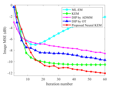
Fig. 6(a) and Fig. 6(b) further show image MSE as a function of iteration number for the two different frames (frame 2 and frame 12). For the DIP reconstruction, the ADMM algorithm demonstrated a relatively faster convergence rate in early iterations than the KEM and DIP by OT. This is mainly because four sub-iterations were used for the tomographic reconstruction step in the ADMM algorithm while one sub-iteration was used for other algorithms. The DIP by OT was either comparable to (Fig. 6(b)) or better than (Fig. 6(a)) the DIP by ADMM. Note that here the DIP by ADMM and DIP by OT were not always close to each other. This can be explained by that the neural network model is nonlinear and different algorithms are not guaranteed to provide the same solution.

Fig. 6(c) shows the plots of image MSE for all time frames reconstructed by different methods with 60 iterations. Error bars were calculated over 10 noisy realizations. The DIP by ADMM showed a slightly unstable behavior across different frames. This is likely because a single value of the hyper-parameter $\rho$ has varying efficacy for different time frames. The regular KEM was either equivalent to or slightly better than the DIP by OT. The proposed neural KEM further improved all the frames as compared to the regular KEM.

Fig. 7 shows the trade-off between the bias and SD of different methods for ROI quantification in the blood and tumor regions. The two ROIs are the same as the anatomical regions marked in Fig. 4a. The curves were obtained by varying the iteration number from 10 to 60 iterations with an interval of 10 iterations. As expected, the bias decreases as the iteration number increases in all the methods. For the blood ROI quantification, the DIP by OT was better than the DIP by ADMM because of the improved convergence and stability by OT in these three cases. For the tumor ROI quantification, the DIP by OT was either better than the DIP by ADMM in the low and medium cases (frame 2 and frame 12) or comparable in the high-count case (frame 24).

The proposed neural KEM achieved the lowest SD and bias simultaneously for frame 2 and frame 12 after 20 iterations, demonstrating its advantage for low- and medium-count frames. In the high-count case (frame 24), the traditional ML-EM achieved the lowest bias for small targets (i.e., the tumor and blood ROIs) due to a good recovery of the contrast at a high iteration number. The neural KEM was with a higher bias due to oversmoothness in this high-count case but it was still better than the regular KEM and DIP methods.

To demonstrate the challenge for choosing a proper ADMM parameter $\rho$ in the DIP method, Fig. 8(a) shows the iteration-based MSE result for a range of $\rho$ values for frame 12. An inappropriate $\rho$ resulted in instability and oscillations across iterations. $\rho=0.05$ was a good choice for this frame but resulted in poor MSE for some of other frames, as shown in Fig. 6(c). The OT algorithm avoids this difficult-to-tune parameter.

Similar to other methods that use neural network-based deep prior, the proposed neural KEM involves a sub-iteration number that needs to be determined for the neural-network learning step. Fig. 8(b) shows the effect of this sub-iteration number on the final image MSE for frame 2 (low-count), frame 12 (medium-count) and frame 24 (high-count). The result suggests a reasonable choice is 150 iterations, which also worked well for other frames. We also found that the CNN training is stable when the learning rate in the Adam optimizer ranges from 10^-4 to 10^-2.

We also performed a fully-3D computer simulation study using an XCAT heart phantom for a GE Discovery 690 PET scanner. This scanner has 13,824 LYSO crystals, arranged in 24 ring detectors. The detection unit is composed of blocks consisting of 9$\times$6 crystals, each containing a total of 64 blocks per ring. The sinogram size is $381\times 553\times 288$ and the image size is $137\times 137\times 47$. The voxel size was $4.0\times 4.0\times 3.3$ mm³. A one-hour dynamic ¹⁸F-FDG scan was simulated using 49 time frames: 30$\times$10s, 10$\times$60s, and 9$\times$300s. Here the framing scheme is adapted to capture the fast kinetics in the heart. The TACs of different regions were extracted from a real patient FDG PET scan to generate noise-free dynamic activity images. The images were then forward projected to generate noise-free sinograms. No time-of-flight information was simulated. To reduce time, SimSET-based simulation was not used for scatter simulation here. Instead, scattered and random events were simulated using a 40% uniform sinogram. Poisson noise was then generated with 1.25 billion expected events over 1 hour. Ten noisy realizations were simulated.

For the kernel methods, the kernel matrix $\bm{K}$ was built using four composite frames (one 5-min frame, one 15-min frame and two 20-min frames). Here compared to the 3 composite frames used for the 2D simulation study, the first 20-min was divided into two shorter composite frames to better capture the early dynamic information for reconstructing the data of higher temporal resolution. The kNN search was performed in a $9\times 9\times 9$ local region with $k=50$ nearest neighbors to reduce the computation time. The 3D version of U-net was used in the neural network-based methods with the 4 composite images as the network input. Similar to the 2D simulation study, 150 iterations were used for the neural-network learning step within each outer iteration. The proposed neural KEM was compared with ML-EM, regular KEM and DIP by OT using the image MSE and ROI bias-SD metrics. All the methods were run for 60 iterations starting from a uniform initial image.

Fig. 9 shows the true 3D activity images and reconstructed images at iteration 60 by different reconstruction methods for frame 6 (early 10-s frame, low-count level) and frame 49 (late 5-min frame, high-count level). The proposed neural KEM achieved the lowest image MSE for both frames.

Fig. 10(a) shows the plots of image MSE for all frames reconstructed by different methods with 60 iterations. The two kernel-based methods (regular KEM and neural KEM) demonstrated a substantial improvement as compared to the ML-EM and DIP methods. The neural KEM was further better than the regular KEM particularly for those low-count frames.

Fig. 10(b) and fig. 10(c) show the trade-off between the bias and SD of different methods for ROI quantification in an aorta ROI of 3077 voxels and a myocardium ROI of 3744 voxels, respectively. The result of this 3D simulation study here is consistent with that of the 2D simulation study. The DIP method demonstrated a poor ROI bias-SD performance for the myocardial ROI quantification even though the associated image MSE was better than the MLEM. In comparison, the proposed neural KEM achieved the best trade-off among the different reconstruction methods.

We have further applied the neural KEM to dynamic PET imaging for a real patient dataset. A cancer patient scan was performed on the GE Discovery 690 PET/CT scanner at the UC Davis Medical Center. The PET scan started right at the injection of 10 mCi ¹⁸F-FDG and lasted 60 minutes. As our simulation studies have indicated that the neural KEM mainly benefits low-count frames, here we focus on high-temporal resolution dynamic imaging. The one-hour data are divided into 97 time frames following the schedule $60\times 2$s, $18\times 10$s, $10\times 60$s, and $9\times 300$s. A CT scan was acquired for attenuation correction. The projection data size was $381\times 553\times 288$ and the image size was $192\times 192\times 47$. All data corrections, including normalization, attenuation correction, scatter correction and random correction, were extracted using the vendor software and included in the reconstruction process. Similar to the 3D simulation study, four composite frames (one 5-min frame, one 15-min frame and two 20-min frames)) were used to build the kernel matrix for this high-temporal resolution reconstruction. Other algorithm settings were also the same as used for the 3D simulation study described in Section V.A.

For ROI analyses, three ROIs were manually drawn on the corresponding CT images in the descending aorta, the tumor, and the kidney cortex regions. The volume of the blood ROI, tumor ROI and kidney ROI is 9 cm³, 12 cm³, and 15 cm³, respectively.

Fig. 11 shows the comparison of different reconstructions for a late 5-minute frame ($t=3300-3600s$) and two early 2-s frames ($t=18-20s$, $t=36-38s$). Each reconstruction is shown in the transverse and coronal views.

For the 5-minute frame which has a relatively high count level, the ML-EM reconstruction had good contrast in the tumor region though still contained high noise in the normal liver parenchyma. The DIP by OT caused over-smoothness and demonstrated a distortion in the tumor as pointed by the arrow in Fig. 11(a). With a preserved tumor shape similar to that of the ML-EM, both the regular KEM and neural KEM suppressed noise well and provided similar results in this high-count reconstruction, though the latter may have a slightly higher risk of oversmoothing small targets or sharp edges for higher count data due to the additional regularization from the use of deep coefficient prior.

For the 2-s frames, the ML-EM reconstructions were extremely noisy. The DIP by OT significantly reduced noise but tended to over-smooth the images. In Fig. 11(b), KEM resulted in a discontinuous aorta while the proposed neural KEM showed a more natural shape. In Fig. 11(c), the neural KEM also showed a more continuous renal cortex, which may benefit parametric imaging as will be presented in the next subsection. To sum up, the proposed neural KEM not only suppressed the noise in the background regions but also preserved structural contrast and details, though it cannot exclude a potential risk of over-regularization similar to any other methods that includes a regularization. Here the neural KEM and DIP by OT showed different anatomical structures in these two low-count frames. While there is no ground truth and the ML-EM was too noisy to provide a reference, the result from the high-count frame shown in Fig. 11(a) may imply the result by the neural KEM is more likely to be close to the truth of the low-count frames.

Fig. 12 further shows a quantitative comparison of different methods for ROI quantification in the blood ROI in frame 15 (where the uptake in the blood reaches its maximum), and in the tumor ROI and kidney ROI in the last frame (55-60 min). Here the ROI mean is plotted versus normalized background noise SD by varying the iteration number from 10 to 60. The proposed neural KEM achieved the best trade-off among all the other methods.

Parametric imaging was also performed for the dynamic images of the same subject. Because different reconstruction methods mainly make a difference for early-time frames which have a low count level (Fig. 11), here we focused on parametric imaging of early-dynamic data. A two-tissue compartment model with voxel-wise time delay estimation [41] was used to generate parametric images from the early-dynamic data. For each reconstruction method, the blood input function was derived from the descending aorta ROI.

Fig. 13 shows the parametric images of fractional blood volume $v_{b}$ and FDG delivery rate $K_{1}$ generated from the early 120s data. The CT images are also shown for reference of anatomy. The ML-EM result suffered from heavy noise. The KEM result demonstrated a significant improvement but still suffered from noise-induced artifacts. The proposed neural KEM showed more complete and regular kidney cortex structures that seem consistent with the kidney anatomy and function [42]. The $K_{1}$ by DIP was much lower in the kidney cortex region, which can be explained by the underestimation of the renal uptake in the DIP-reconstructed activity image as shown in Fig. 11(c) and Fig. 12(c).

References

- [1] J. Qi and R. M. Leahy, “Iterative reconstruction techniques in emission computed tomography,” Phys. Med. Biol., vol. 51, no. 15, pp. R541-R578, Aug. 2006.
- [2] G. B. Wang and J. Qi, “PET image reconstruction using kernel method,” IEEE Trans. Med. Imag., vol. 34, no. 1, pp. 61-71, Jan. 2015.
- [3] G. B. Wang, “High temporal-resolution dynamic PET image reconstruction using a new spatiotemporal kernel method,” IEEE Trans. Med. Imag., vol. 38, no. 3, pp. 664-674, Mar. 2019.
- [4] W. Hutchcroft, G. B. Wang, K. Chen, C. Catana, and J. Qi, “Anatomically-aided PET reconstruction using the kernel method,” Phys. Med. Biol., vol. 61, no. 18, pp. 6668-6683, 2016.
- [5] P. Novosad and A. J. Reader, “MR-guided dynamic PET reconstruction with the kernel method and spectral temporal basis functions,” Phys. Med. Biol., vol. 61, no. 12, pp. 4624-4645, 2016.
- [6] J. Bland et al.,“MR-guided kernel EM reconstruction for reduced dose PET imaging,” IEEE Trans. Radiat. Plasma Med. Sci., vol. 2, no. 3,pp. 235-243, May 2018.
- [7] K. Gong, J. Cheng-Liao, G. B. Wang, K. T. Chen, C. Catana, and J. Qi, “Direct Patlak reconstruction from dynamic PET data using the kernel method with MRI information based on structural similarity,” IEEE Trans. Med. Imag., vol. 37, no. 4, pp. 955-965, Apr. 2018.
- [8] D. Deidda et al., “Hybrid PET-MR list-mode kernelized expectation maximization reconstruction,” Inverse. Probls., vol. 35, no. 4, pp. 044001, 2019.
- [9] D. Deidda et al., “Effect of PET-MR inconsistency in the kernel image reconstruction method,” IEEE Trans. Radiat. Plasma Med. Sci., vol. 3, no. 4, pp. 400-409, July 2019.
- [10] X. Zhang et al., “Total-body dynamic reconstruction and parametric imaging on the uEXPLORER,” J. Nucl. Med., vol. 61, no. 2, pp. 285-291, 2020.
- [11] D. L. Snyder and M. I. Miller, “The use of sieves to stabilize images produced with the EM algorithm for emission tomography,” IEEE Trans. Nucl. Sci. vol. 32, no. 5, pp. 3864-3872, Oct. 1985.
- [12] J. E. Bowsher, V. E. Johnson, T. G. Turkington, R. J. Jaszczak, C. E. Floyd, and R. E. Coleman, “Bayesian reconstruction and use of anatomical a priori information for emission tomography,” IEEE Trans. Med. Imag., vol. 15, no. 5, pp. 673-686, Oct. 1996.
- [13] C. Chan, R. Fulton, D. D. Feng, and S. Meikle, “Regularized image reconstruction with an anatomically adaptive prior for positron emission tomography,” Phys. Med. Biol., vol. 54, no. 24, pp. 7379-400, 2009.
- [14] J. Cheng-Liao and J. Qi, “PET image reconstruction with anatomical edge guided level set prior,” Phys. Med. Biol., vol. 56, no. 21, p. 6899, 2011.
- [15] K. Vunckx et al., “Evaluation of three MRI-based anatomical priors for quantitative PET brain imaging,” IEEE Trans. Med. Imag., vol. 31, no. 3, pp. 599-612, Mar. 2012.
- [16] K. Kim et al., “Penalized PET reconstruction using deep learning prior and local linear fitting,” IEEE Trans. Med. Imag., vol. 37, no. 6, pp. 1478-1487, Jun. 2018.
- [17] N. Xie et al., “Penalized-likelihood PET image reconstruction using 3D structural convolutional sparse coding,” IEEE Trans. Bio-Med. Eng., vol. 69, no. 1, pp. 4-14, Jan. 2022.
- [18] K. Gong, C. Catana, J. Y. Qi, and Q. Z. Li, “PET image reconstruction using deep image prior,” IEEE Trans. Med. Imag., vol. 38, no. 7, pp. 1655-1665, Jul. 2019.
- [19] K. Gong et al., “Iterative PET image reconstruction using convolutional neural network representation,” IEEE Trans. Med. Imag., vol. 38, no. 3, pp. 675-685, Mar. 2019.
- [20] K. Gong, C. Catana, J. Qi and Q. Li, “Direct reconstruction of linear parametric images from dynamic PET using nonlocal deep image prior,” IEEE Trans. on Med. Imag., vol. 41, no. 3, pp. 680-689, Mar. 2022.
- [21] Z. Xie et al., “Generative adversarial network based regularized image reconstruction for PET,” Phys. Med. Biol., vol. 65, no. 12, pp. 125016, 2020.
- [22] T. Yokota, K. Kawai, M. Sakata, Y. Kimura, and H. Hontani, “Dynamic PET image reconstruction using nonnegative matrix factorization incorporatedwith deep image prior,” in Proc. IEEE Int. Conf. Comput. Vis., 2019.
- [23] Z. Xie, T. Li, X. Zhang, W. Qi, E. Asma, and J. Qi, “Anatomically aided PET image reconstruction using deep neural networks,” Med. Phys., vol. 48, no. 9, pp. 5244-5258, Sep. 2021.
- [24] D. Ulyanov, A. Vedaldi, and V. Lempitsky, “Deep image prior,” Int. J. Comput. Vis., vol. 128, no. 7, pp. 1867-1888, 2020.
- [25] G. B. Wang, and J. Qi, “Iterative nonlinear least squares algorithms for direct reconstruction of parametric images from dynamic PET,” IEEE ISBI, 2008, pp. 1031-1034.
- [26] G. B. Wang, and J. Qi, “An optimization transfer algorithm for nonlinear parametric image reconstruction from dynamic PET data,” IEEE Trans. on Med. Imag., vol. 31, no. 10, pp. 1977-1986, Oct. 2012.
- [27] J. A. Fessler, “Optimization transfer approach to joint registration / reconstruction for motion-compensated image reconstruction,” IEEE ISBI, 2010, pp. 596-599.
- [28] K. Lange, D. R. Hunter, and I. Yang, “Optimization transfer using surrogate objective functions,” J. Comput. Graphical Stat., vol. 9, no. 1, pp. 1-20, 2000.
- [29] A. J. Reader, G. Corda, A. Mehranian, C. Costa-Luis, S. Ellis, and J. A. Schnabel, “Deep learning for PET image reconstruction,” IEEE Trans. Radiat. Plasma Med. Sci., vol. 5, no. 1, pp. 1-24, Jan., 2021.
- [30] K. Gong, E. Berg, S. R. Cherry and J. Qi, “Machine learning in PET: From photon detection to quantitative image reconstruction,” Proc. IEEE Inst. Electr. Electron. Eng., vol. 108, no. 1, pp. 51-68, Jan., 2020.
- [31] T. Wang et al., “Machine learning in quantitative PET: A review of attenuation correction and low-count image reconstruction methods,” Phys. Med., vol. 76, pp. 294-306, 2020.
- [32] G. Wang, J. Ye, and B. De Man, “Deep learning for tomographic image reconstruction,” Nat. Mach. Intell., vol. 2, pp. 737-748, 2020.
- [33] G. Wang, M. Jacob, X. Mou, Y. Shi, and Y. C. Eldar, “Deep tomographic image reconstruction: yesterday, today, and tomorrow—editorial for the 2nd special issue “Machine Learning for Image Reconstruction”,” IEEE Trans. Med. Imag., vol. 40, no. 11, pp. 2956-2964, Nov., 2021.
- [34] I. Hggstrm, C. R. Schmidtlein, G. Campanella, and T. J. Fuchs, “DeepPET: A deep encoder-decoder network for directly solving the PET image reconstruction inverse problem,” Med. Imag. Anal., vol. 54, pp. 253–262, May 2019.
- [35] H. Lim, I. Y. Chun, Y. K. Dewaraja, and J. A. Fessler, “Improved low-count quantitative PET reconstruction with an iterative neural network”, IEEE Trans. Med. Imag., vol. 39, no. 11, pp. 3512-3522, Nov. 2020.
- [36] A. Mehranian and A. J. Reader, “Model-based deep learning PET image reconstruction using forward-backward splitting expectation maximisation,” IEEE Trans. Radiat. Plasma Med. Sci., vol. 5, no. 1, pp. 54-64, Jan. 2021.
- [37] L. A. Shepp and Y. Vardi, “Maximum likelihood reconstruction for emission tomography,” IEEE Trans. Med. Imag., vol. MI-1, no. 2, pp. 113-122, Oct., 1982.
- [38] J. H. Friedman, J. Bentely, and R. A. Finkel, “An algorithm for finding best matches in logarithmic expected time,” ACM Trans. Math. Software, vol. 3, no. 3, pp. 209-226, 1977.
- [39] R. L. Harrison et al., “Preliminary experience with the photon history generator module of a public-domain simulation system for emission tomography,” in Conf. Rec. IEEE Nucl. Sci. Symp. Med. Imag. Conf., pp. 1154-11581, 1993.
- [40] Z. Ashouri, G. B. Wang, R. M. Dansereau and R. A. de Kemp, “Evaluation of wavelet kernel-based PET image reconstruction,” IEEE Trans. Radiat. Plasma Med. Sci., vol. 6, no. 5, pp. 564-573, May 2022.
- [41] G. B. Wang et al., “Total-body PET multiparametric imaging of cancer using a voxel-wise strategy of compartmental modeling,” J. Nucl. Med., vol. 63, no. 8, pp. 1274-1281, 2022.
- [42] C. Ruiz-Bedoya et al., “11C-PABA as a PET radiotracer for functional renal imaging: Preclinical and first-in-human study,” J. Nucl. Med., vol. 61, no. 11, pp. 1665-1671, 2020.
- [43] S. Li and G. B. Wang, “Modified kernel MLAA using autoencoder for PET-enabled dual-energy CT,” Philos. Trans. Royal Soc. A, vol. 379, no. 2204, 2021.
- [44] S. Li and G. B. Wang, “Deep kernel representation for image reconstruction in PET,” IEEE Trans. Med. Imag., early access, 2022, doi: 10.1109/TMI.2022.3176002.
- [45] S. Cherry, R. Badawi, J. Karp, W. Moses, P. Price, and T. Jones, “Total-body imaging: Transforming the role of PET in translational medicine,” Sci. Transl. Med., vol. 9, no. 381, p. eaaf6169, 2017.
- [46] R. Badawi et al., “First human imaging studies with the EXPLORER total-body PET scanner,” J. Nucl. Med., vol. 60, no. 3, pp. 299-303, 2019.
- [47] B. Spencer et al., “Performance evaluation of the uEXPLORER total-body PET/CT scanner based on NEMA NU 2-2018 with additional tests to characterize PET scanners with a long axial field of view,” J. Nucl. Med., vol. 62, no.6, pp. 861-870, 2021.
- [48] J. Karp et al., “Imaging performance of the PennPET Explorer scanner,” J. Nucl. Med., 59: 222-222, 2018.
- [49] A. Pantel et al., “PennPET Explorer: Human imaging on a whole-body imager,” J. Nucl. Med., vol. 61, no. 1, pp. 144-151, 2020.