Neural Gradient Learning and Optimization for Oriented Point Normal Estimation

Qing Li School of Software, Tsinghua UniversityBeijingChina [email protected] , Huifang Feng School of Informatics, Xiamen UniversityXiamenChina [email protected] , Kanle Shi Kuaishou TechnologyBeijingChina [email protected] , Yi Fang Center for Artificial Intelligence and Robotics, New York UniversityAbu DhabiUAE [email protected] , Yu-Shen Liu School of Software, Tsinghua UniversityBeijingChina [email protected] and Zhizhong Han Department of Computer Science, Wayne State UniversityDetroitUSA [email protected]

(2023)

Abstract.

We propose Neural Gradient Learning (NGL), a deep learning approach to learn gradient vectors with consistent orientation from 3D point clouds for normal estimation. It has excellent gradient approximation properties for the underlying geometry of the data. We utilize a simple neural network to parameterize the objective function to produce gradients at points using a global implicit representation. However, the derived gradients usually drift away from the ground-truth oriented normals due to the lack of local detail descriptions. Therefore, we introduce Gradient Vector Optimization (GVO) to learn an angular distance field based on local plane geometry to refine the coarse gradient vectors. Finally, we formulate our method with a two-phase pipeline of coarse estimation followed by refinement. Moreover, we integrate two weighting functions, i.e., anisotropic kernel and inlier score, into the optimization to improve the robust and detail-preserving performance. Our method efficiently conducts global gradient approximation while achieving better accuracy and generalization ability of local feature description. This leads to a state-of-the-art normal estimator that is robust to noise, outliers and point density variations. Extensive evaluations show that our method outperforms previous works in both unoriented and oriented normal estimation on widely used benchmarks. The source code and pre-trained models are available at https://github.com/LeoQLi/NGLO.

Geometric Deep Learning, Point Clouds, Normal Estimation, Neural Gradient, Surface Reconstruction

^†^†journalyear: 2023^†^†copyright: acmlicensed^†^†conference: SIGGRAPH Asia 2023 Conference Papers; December 12–15, 2023; Sydney, NSW, Australia^†^†booktitle: SIGGRAPH Asia 2023 Conference Papers (SA Conference Papers ’23), December 12–15, 2023, Sydney, NSW, Australia^†^†price: 15.00^†^†doi: 10.1145/3610548.3618253^†^†isbn: 979-8-4007-0315-7/23/12^†^†ccs: Computing methodologies Point-based models^†^†ccs: Computing methodologies Mesh models^†^†ccs: Computing methodologies Reconstruction

1. Introduction

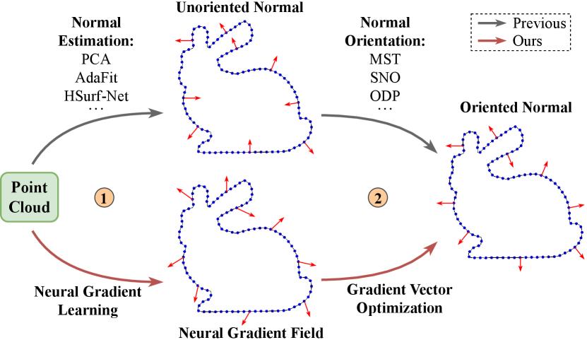
Refer to caption — Figure 1. For oriented normal estimation, previous methods usually conduct a two-stage pipeline, i.e., (1) unoriented normal estimation and (2) normal orientation, while our method achieves this through Neural Gradient Learning (NGL) and Gradient Vector Optimization (GVO). We introduce effective novel designs into our method that enable it to improve the SOTA results.

Normal estimation is a fundamental task in computer vision and computer graphics. Oriented normal with consistent orientation is a prerequisite for many downstream tasks, such as graphics rendering (Blinn, 1978; Gouraud, 1971; Phong, 1975) and surface reconstruction (Kazhdan, 2005; Kazhdan et al., 2006; Kazhdan and Hoppe, 2013). Due to noise levels, uneven sampling densities, and various complex geometries, estimating oriented normals from 3D point clouds still remains challenging. As shown in Fig. 1, the paradigm of oriented normal estimation usually includes: unoriented normal estimation that provides vectors perpendicular to the surfaces defined by local neighborhoods; normal orientation that aligns the directions of adjacent vectors for global consistency. Over the past few years, many excellent algorithms (Lenssen et al., 2020; Ben-Shabat and Gould, 2020; Zhu et al., 2021; Li et al., 2022b, a, 2023b) have been proposed for unoriented normal estimation. However, their estimated normals are randomly oriented on both sides of the surface and cannot be directly used in downstream applications without normal orientation. Most normal orientation approaches are based on a propagation strategy (Hoppe et al., 1992; König and Gumhold, 2009; Schertler et al., 2017; Xu et al., 2018; Jakob et al., 2019; Metzer et al., 2021). These methods are mainly based on the assumption of smooth and clean points, and carefully tune data-specific parameters, such as the neighborhood size of the propagation. Moreover, the issue of error propagation in the orientation process may let errors in local areas overflow into the subsequent steps.

The two-stage architecture of existing oriented normal estimation paradigms needs to combine two independent algorithms, and requires a lot of work to tune the parameters of the two algorithms. More importantly, the stability and effectiveness of the integrated algorithm cannot be guaranteed. In our experiments, we evaluate the combinations of different algorithms for unoriented normal estimation and normal orientation. A key observation is that, for the same normal orientation algorithm, integrating a better unoriented normal estimation algorithm does not lead to better orientation results. That is, using higher precision unoriented normals does not necessarily result in more accurate oriented normals using existing propagation strategies. In Fig. 2, we use a simple example to illustrate that judging whether to invert the direction of neighborhood normals based on a propagation rule will lead to unreasonable results. The propagation strategy is affected by the direction distribution of the unoriented normal vectors. Therefore, it is necessary to design a complete and unified pipeline for oriented normal estimation.

In a data-driven manner, the workflow of our proposed method is an inversion of the traditional pipeline (see Fig. 1). We start by solving normals with consistent orientation but possibly moderate accuracy, and then we further refine the normals. We introduce Neural Gradient Learning (NGL) and Gradient Vector Optimization (GVO), defined by a family of loss functions that can be used with point cloud data with noise, outliers and point density variations, and efficiently produce high accurate oriented normals for each point. Specifically, the NGL learns gradient vectors from global geometry representation, while the GVO optimizes vectors based on an insight into the local property. A series of qualitative and quantitative evaluation experiments are conducted to demonstrate the effectiveness of the proposed method.

To summarize, our main contributions include:

•

A technique of neural gradient learning, which can derive gradient vectors with consistent orientations from implicit representations of point cloud data.
•

A gradient vector optimization strategy, which learns an angular distance field based on local geometry to further optimize the gradient vectors.
•

We report the state-of-the-art performance for both unoriented and oriented normal estimation on point clouds with noise, density variations and complex geometries.

2. Related Work

2.1. Unoriented Normal Estimation

The most widely used unoriented normal estimation method for point clouds is Principle Component Analysis (PCA) (Hoppe et al., 1992). Later, PCA variants (Alexa et al., 2001; Pauly et al., 2002; Mitra and Nguyen, 2003; Lange and Polthier, 2005; Huang et al., 2009), Voronoi-based paradigms (Amenta and Bern, 1999; Mérigot et al., 2010; Dey and Goswami, 2006; Alliez et al., 2007), and methods based on complex surfaces (Levin, 1998; Cazals and Pouget, 2005; Guennebaud and Gross, 2007; Aroudj et al., 2017; Öztireli et al., 2009) have been proposed to improve the performance. These traditional methods (Hoppe et al., 1992; Cazals and Pouget, 2005) are usually based on geometric prior of point cloud data itself, and require complex preprocessing and parameter fine-tuning according to different types of data. Recently, some studies proposed to use neural networks to directly or indirectly map high-dimensional features of point clouds into 3D normal vectors. For example, the regression-based methods directly estimate normals from structured data (Boulch and Marlet, 2016; Roveri et al., 2018; Lu et al., 2020) or unstructured point clouds (Guerrero et al., 2018; Zhou et al., 2020b; Hashimoto and Saito, 2019; Ben-Shabat et al., 2019; Zhou et al., 2020a, 2022; Li et al., 2022a, 2023b). In contrast, the surface fitting-based methods first employ a neural network to predict point weights, then they derive normal vectors through weighted plane fitting (Lenssen et al., 2020; Cao et al., 2021) or polynomial surface fitting (Ben-Shabat and Gould, 2020; Zhu et al., 2021; Zhou et al., 2023; Zhang et al., 2022; Li et al., 2022b) on local neighborhoods. In our experiments, we observe that regression-based methods train models more stably and perform optimization more efficiently without coupling the fitting step used in fitting-based methods. In contrast, our method finds the optimal point normal through a classification strategy.

2.2. Consistent Normal Orientation

The normals estimated by the above methods do not preserve a consistent orientation since they only look for lines perpendicular to the surface. Based on local consistency strategy, the pioneering work (Hoppe et al., 1992) and its improved methods (Seversky et al., 2011; Wang et al., 2012; Schertler et al., 2017; Xu et al., 2018; Jakob et al., 2019) propagate seed point’s normal orientation to its adjacent points via a Minimum Spanning Tree (MST). More recent work (Metzer et al., 2021) introduces a dipole propagation strategy across the partitioned patches to achieve global consistency. However, these methods are limited by error propagation during the orientation process. Some other methods show that normal orientation can benefit from reconstructing surfaces from unoriented points. They usually adopt different volumetric representation techniques, such as signed distance functions (Mullen et al., 2010; Mello et al., 2003), variational formulations (Walder et al., 2005; Huang et al., 2019; Alliez et al., 2007), visibility (Katz et al., 2007; Chen et al., 2010), isovalue constraints (Xiao et al., 2023), active contours (Xie et al., 2004) and winding-number field (Xu et al., 2023). The correctly-oriented normals can be achieved from their solved representations, but their normals are not accurate in the vertical direction. Furthermore, a few approaches (Guerrero et al., 2018; Hashimoto and Saito, 2019; Wang et al., 2022; Li et al., 2023a) focus on using neural networks to directly learn a general mapping from point clouds to oriented normals. Different from the above methods, we solve the oriented normal estimation by first determining the global orientation and then improving its direction accuracy based on local geometry.

3. Preliminary

In general, the gradient of a real-valued function $f(x,y,z)$ in a 3D Cartesian coordinate system (also called gradient field) is given by a vector whose components are the first partial derivatives of $f$ , i.e., $\nabla f(x,y,z)\!=\!{f_{x}}\bm{i}+{f_{y}}\bm{j}+{f_{z}}\bm{k}$ , where $\bm{i},\bm{j}$ and $\bm{k}$ are the standard unit vectors in the directions of the $x,y$ and $z$ coordinates, respectively. If the function $f$ is differentiable at a point $\bm{p}$ and suppose that $\nabla f(\bm{p})\!\neq\!0$ , then there are two important properties of the gradient field: (1) The maximum value of the directional derivative, i.e., the maximum rate of change of the function $f$ , is defined by the magnitude of the gradient $\left\|\nabla f\right\|$ and occurs in the direction given by $\nabla f$ . (2) The gradient vector $\nabla f$ is perpendicular to the level surface $f(\bm{p})\!=\!0$ .

Recently, deep neural networks have been used to reconstruct surfaces from point cloud data by learning implicit functions. These approaches represent a surface as the zero level-set of an implicit function $f$ , i.e.,

(1)

\mathcal{S}=\left\{\bm{x}\in\mathbb{R}^{3}~{}|~{}f(\bm{x};\bm{\theta})=0\right\},

where $f\colon\mathbb{R}^{3}\!\rightarrow\!\mathbb{R}$ is a neural network with parameter $\bm{\theta}$ , such as multi-layer perceptron (MLP). Implicit function learning methods adopt either signed distance function (Park et al., 2019) or binary occupancy (Mescheder et al., 2019) as the shape representation. If the function $f$ is continuous and differentiable, the formula of normal vector (perpendicular to the surface) at a point $\bm{p}$ is $\bm{n}_{\bm{p}}\!=\!\nabla f(\bm{p})/\left\|\nabla f(\bm{p})\right\|$ , where $\|\!\cdot\!\|$ means vector norm. Using neural networks as implicit representations of surfaces can benefit from their adaptability and approximation capability (Atzmon et al., 2019). Meanwhile, we can obtain the gradient $\nabla f$ in the back-propagation process of training $f$ .

4. Method

As shown in Fig. 3, our method consists of two parts: (1) the neural gradient learning $(\bm{P}\!\rightarrow\!f\!\rightarrow\!\nabla f)$ to estimate inaccurate but correctly-oriented gradients, and (2) the gradient vector optimization $(\nabla f\!\rightarrow\!g\!\rightarrow\!\bm{n})$ to refine the coarse gradients to obtain accurate normals, which will be introduced in the following sections.

4.1. Neural Gradient Learning

Consider a point set $\bm{X}\!=\!\{\bm{x}_{i}\}_{i=1}^{M_{1}}$ that is sampled from raw point cloud $\bm{P}$ (possibly distorted) through certain probability distribution $\mathcal{D}$ , we explore training a neural network $f$ with parameter $\bm{\theta}$ to derive the gradient during the optimization. First, we introduce a loss function defined by the form of

(2)

\mathcal{L}(\bm{\theta})=\mathbb{E}_{\bm{x}\sim\mathcal{D}}~{}\mathcal{T}\big{(}F(\bm{x};\bm{\theta}),\mathcal{F}_{\bm{X}}(\bm{x})\big{)}~{},

where $\mathcal{T}\colon\mathbb{R}\times\mathbb{R}\rightarrow\mathbb{R}$ is a differentiable similarity function. $F(\bm{x};\bm{\theta})$ is the learning objective to be optimized and $\mathcal{F}_{\bm{X}}(\bm{x})$ is the distance measure with respect to $\bm{X}$ . In this work, our insight is that incorporating neural gradients in a manner similar to (Atzmon and Lipman, 2020, 2021) can learn neural gradient fields with consistent orientations from various point clouds. To this end, we add the derivative data of $f$ , i.e.,

(3)

F(\bm{x};\bm{\theta})=f(\bm{x};\bm{\theta})\cdot\bm{v}~{},

where $\bm{v}\!=\!\nabla f(\bm{x};\bm{\theta})/\left\|\nabla f(\bm{x};\bm{\theta})\right\|$ is the normalized neural gradient. Eq. (3) incorporates an implicit representation and a gradient approximation with respect to the underlying geometry of $\bm{X}$ .

We first show a special case of Eq. (2), which is given by

(4)

\mathcal{L}(\bm{\theta})=\mathbb{E}_{\bm{x}\sim\mathcal{D}}~{}\mathcal{T}\big{(}\bm{x}-f(\bm{x};\bm{\theta})\cdot\bm{v},~{}\bm{p}\big{)}.

Such definition of training objective has been used by surface reconstruction methods (Ma et al., 2021; Chibane et al., 2020) to learn signed or unsigned distance functions from noise-free data. Recall that the gradient will be the direction in which the distance value increases the fastest. These methods exploit this property to move a query position $\bm{x}$ by distance $f(\bm{x};\bm{\theta})$ along or against the gradient direction $\bm{v}$ to its closest point $\bm{p}$ sampled on the manifold. Specifically, $f(\bm{x};\bm{\theta})$ is interpreted as a signed distance (Ma et al., 2021) or unsigned distance (Chibane et al., 2020). This way they can learn reasonable signed/unsigned distance functions from the input noise-free point clouds. In contrast, we are not looking to learn an accurate distance field to approximate the underlying surface, but to learn a neural gradient field with a consistent orientation from a variety of data, even in the presence of noise.

Next, we will extend Eq. (2) to a more general case for neural gradient learning. Given a point $\bm{x}$ , instead of using the unsigned distance in (Atzmon and Lipman, 2020) or its nearest sampling point (Ma et al., 2021; Chibane et al., 2020), we consider the mean vector of its neighborhood, that is

(5)

\mathcal{F}_{\bm{X}}(\bm{x})=\frac{1}{k}\sum_{i=1}^{k}\big{(}\bm{x}-\mathcal{N}^{k}_{i}(\bm{x},\bm{P})\big{)},~{}\bm{x}\in\bm{X}~{},

where $\mathcal{N}^{k}_{i}(\bm{x},\bm{P})$ denotes the $k$ nearest points of $\bm{x}$ in $\bm{P}$ . Intuitively, $\mathcal{F}_{\bm{X}}(\bm{x})\!\in\!\mathbb{R}^{3}$ is a vector from the averaged point position $\bar{\bm{x}}\!=\!\sum_{i=1}^{k}\mathcal{N}^{k}_{i}(\bm{x},\bm{P})/k$ to $\bm{x}$ .

For the similarity measure $\mathcal{T}$ of vector-valued functions, we adopt the standard Euclidean distance. Then, the loss in Eq. (2) for Neural Gradient Learning (NGL) has the format

(6)

\mathcal{L}(\bm{\theta})=\left\|f(\bm{x};\bm{\theta})\cdot\bm{v}-\frac{1}{k}\sum_{i=1}^{k}\big{(}\bm{x}-\mathcal{N}^{k}_{i}(\bm{x},\bm{P})\big{)}\right\|.

As illustrated in Fig. 3(b), our method not only matches the predicted gradient on the position of $\bm{x}$ , but also matches the gradient on the neighboring regions of $\bm{x}$ . This is important because our input point cloud is noisy and individual points may not lie on the underlying surface. Finally, the training loss is an aggregation of the objective for each neural gradient learning function $\mathcal{L}(\bm{\theta})|_{\bm{x}_{i}}$ of $\bm{x}_{i}$ , i.e.,

(7)

\mathcal{L}_{\text{NGL}}=\frac{1}{M_{1}}\sum_{i=1}^{M_{1}}\mathcal{L}(\bm{\theta})|_{\bm{x}_{i}}~{},~{}\bm{x}_{i}\in\bm{X}.

For the distribution $\mathcal{D}$ , we make it concentrate in the neighborhood of $\bm{x}$ in 3D space. Specifically, $\mathcal{D}$ is set by uniform sampling points $\bm{x}$ from $\bm{P}$ and placing an isotropic Gaussian $N(\bm{x},\sigma^{2})$ for each $\bm{x}$ . The distribution parameter $\sigma$ depends on each point $\bm{x}$ and is adaptively set to the distance from the $50$ th nearest point to $\bm{x}$ (Atzmon and Lipman, 2020, 2021).

Our network architecture for neural gradient learning is based on the one used in (Atzmon and Lipman, 2020; Ma et al., 2021), which is composed of eight linear layers with ReLU activation functions (except the last layer) and a skip connection. After training, the network can derive pointwise gradients from the raw data $\bm{P}$ (see 2D examples in Fig. 4).

Extension. If we assume the raw data $\bm{P}$ is noise-free, that is, the neighbors $\mathcal{N}^{k}(\bm{x},\bm{P})$ are located on the surface, then the formula of Eq. (6) can take another form

(8)

\mathcal{L}(\bm{\theta})=\left\|\big{(}f(\bm{x};\bm{\theta})\cdot\bm{v}-\bm{x}\big{)}+\frac{1}{k}\sum_{i=1}^{k}\mathcal{N}^{k}_{i}(\bm{x},\bm{P})\right\|.

More particularly, if we set $k\!=\!1$ and the nearest point of $\bm{x}$ in $\bm{P}$ be $\bm{p}$ , i.e., $\mathcal{N}^{k=1}(\bm{x},\bm{P})\!=\!\bm{p}$ , then the above formula is turned into the special case in Eq. (4). Specifically, the derived formula in Eq. (8) also distinguishes our method from the methods (Ma et al., 2021; Chibane et al., 2020; Atzmon and Lipman, 2020, 2021), since their objectives only consider the location of each clean point, while our proposed objective covers the neighborhood of each noisy point to approximate the surface gradients.

4.2. Gradient Vector Optimization

A notable shortcoming of neural gradient learning is that the derived gradient vectors are inaccurate because the implicit function tries to approximate the whole shape surface instead of focusing on fitting local regions. Therefore, the learned gradient vectors are inadequate to be used as surface normals and need to be further refined. Inspired by the implicit surface representations, we define the expected normal as the zero level-set of a function

(9)

\bm{\mathcal{V}}=\left\{\bm{x}\in\mathbb{R}^{3},\bm{v}\in\mathbb{R}^{3}~{}|~{}g(\bm{x},\bm{v};\bm{\vartheta})=0\right\},

where $g\colon\mathbb{R}^{3}\times\mathbb{R}^{3}\rightarrow\mathbb{R}$ is a neural network with parameter $\bm{\vartheta}$ that predicts (unsigned) angular distance field between the normalized gradient vector $\bm{v}$ and the ground-truth normal vector $\bm{\hat{n}}$ (see Fig. 5). Given appropriate training objectives, the zero level-set of $g$ can be a vector cluster describing the normals of point cloud $\bm{P}$ . To this end, we introduce Gradient Vector Optimization (GVO) defined by the form of a loss function

(10)

\mathcal{L}(\bm{\vartheta})=\mathbb{E}_{\bm{v}\sim\mathcal{D^{\prime}}}~{}\mathcal{T}\big{(}g(\bm{x},\bm{v};\bm{\vartheta}),~{}\langle\bm{v},\bm{\hat{n}}\rangle\big{)},

where $\mathcal{D^{\prime}}$ is a probability distribution based on an initial vector $\bm{v}\!\in\!\mathbb{R}^{3}$ . $\langle\cdot\rangle\!\in\![0,\pi]$ means the angular difference between two unit vectors. In contrast to the previous method (Li et al., 2023b), we regress angles using weighted features of the approximated local plane instead of point features from PointNet (Qi et al., 2017). The motivation is that simple angle regression with $g$ fails to be robust to noise or produce high-quality normals.

Given a neighborhood size $m$ , we can construct the input data as the nearest neighbor graph $G\!=\!(\mathcal{N},\mathcal{E})$ , where $(\bm{x},\bm{x}_{j})\!\in\!\mathcal{E}$ is a directed edge if $\bm{x}_{j}$ is one of the $m$ nearest neighbors of $\bm{x}$ . Let $\mathcal{N}^{m}(\bm{x})\!=\!\{\bm{x}_{j}-\bm{x}\}_{j=1}^{m}$ be the centered coordinates of the points in the neighborhood. The standard way to solve for unoriented normal at a point is to fit a plane to its local neighborhood (Levin, 1998), which is described as

(11)

\bm{n}_{i}^{\ast}=\mathop{\text{argmin}}_{\bm{n}}\sum_{\bm{x}_{j}^{\prime}\in\mathcal{N}^{m}(\bm{x}_{i})}\left\|\bm{x}_{j}^{\prime}\cdot\bm{n}\right\|^{2}.

In practice, there are two main issues about the utilizing of Eq. (11) (Lenssen et al., 2020): (i) it acts as a low-pass filter for the data and eliminates sharp details, (ii) it is unreliable if there is noise or outliers in the data. We will show that both issues can be resolved by integrating weighting functions into our optimization pipeline. In short, the preservation of detailed features is achieved by an anisotropic kernel that infers weights of point pairs based on their relative positions, while the robustness to outliers is achieved by a scoring mechanism that weights points according to inlier scores.

Table 1. RMSE of oriented normals on datasets PCPNet and FamousShape.

\ast

means the source code is uncompleted.

Category	PCPNet Dataset							FamousShape Dataset
	Noise				Density			Noise				Density
	None	0.12%	0.6%	1.2%	Stripe	Gradient	Average	None	0.12%	0.6%	1.2%	Stripe	Gradient	Average
PCA+MST (Hoppe et al., 1992)	19.05	30.20	31.76	39.64	27.11	23.38	28.52	35.88	41.67	38.09	60.16	31.69	35.40	40.48
PCA+SNO (Schertler et al., 2017)	18.55	21.61	30.94	39.54	23.00	25.46	26.52	32.25	39.39	41.80	61.91	36.69	35.82	41.31
PCA+ODP (Metzer et al., 2021)	28.96	25.86	34.91	51.52	28.70	23.00	32.16	30.47	31.29	41.65	84.00	39.41	30.72	42.92
AdaFit (Zhu et al., 2021)+MST	27.67	43.69	48.83	54.39	36.18	40.46	41.87	43.12	39.33	62.28	60.27	45.57	42.00	48.76
AdaFit (Zhu et al., 2021)+SNO	26.41	24.17	40.31	48.76	27.74	31.56	33.16	27.55	37.60	69.56	62.77	27.86	29.19	42.42
AdaFit (Zhu et al., 2021)+ODP	26.37	24.86	35.44	51.88	26.45	20.57	30.93	41.75	39.19	44.31	72.91	45.09	42.37	47.60
HSurf-Net (Li et al., 2022a)+MST	29.82	44.49	50.47	55.47	40.54	43.15	43.99	54.02	42.67	68.37	65.91	52.52	53.96	56.24
HSurf-Net (Li et al., 2022a)+SNO	30.34	32.34	44.08	51.71	33.46	40.49	38.74	41.62	41.06	67.41	62.04	45.59	43.83	50.26
HSurf-Net (Li et al., 2022a)+ODP	26.91	24.85	35.87	51.75	26.91	20.16	31.07	43.77	43.74	46.91	72.70	45.09	43.98	49.37
PCPNet (Guerrero et al., 2018)	33.34	34.22	40.54	44.46	37.95	35.44	37.66	40.51	41.09	46.67	54.36	40.54	44.26	44.57
DPGO^∗ (Wang et al., 2022)	23.79	25.19	35.66	43.89	28.99	29.33	31.14	-	-	-	-	-	-	-
SHS-Net (Li et al., 2023a)	10.28	13.23	25.40	35.51	16.40	17.92	19.79	21.63	25.96	41.14	52.67	26.39	28.97	32.79
Ours	12.52	12.97	25.94	33.25	16.81	9.47	18.49	13.22	18.66	39.70	51.96	31.32	11.30	27.69

Table 2. RMSE of unoriented normal on datasets PCPNet and FamousShape.

\ast

means the source code is uncompleted or unavailable.

Category	PCPNet Dataset							FamousShape Dataset
	Noise				Density			Noise				Density
	None	0.12%	0.6%	1.2%	Stripe	Gradient	Average	None	0.12%	0.6%	1.2%	Stripe	Gradient	Average
Jet (Cazals and Pouget, 2005)	12.35	12.84	18.33	27.68	13.39	13.13	16.29	20.11	20.57	31.34	45.19	18.82	18.69	25.79
PCA (Hoppe et al., 1992)	12.29	12.87	18.38	27.52	13.66	12.81	16.25	19.90	20.60	31.33	45.00	19.84	18.54	25.87
PCPNet (Guerrero et al., 2018)	9.64	11.51	18.27	22.84	11.73	13.46	14.58	18.47	21.07	32.60	39.93	18.14	19.50	24.95
Zhou et al.^∗ (Zhou et al., 2020b)	8.67	10.49	17.62	24.14	10.29	10.66	13.62	-	-	-	-	-	-	-
Nesti-Net (Ben-Shabat et al., 2019)	7.06	10.24	17.77	22.31	8.64	8.95	12.49	11.60	16.80	31.61	39.22	12.33	11.77	20.55
Lenssen et al. (Lenssen et al., 2020)	6.72	9.95	17.18	21.96	7.73	7.51	11.84	11.62	16.97	30.62	39.43	11.21	10.76	20.10
DeepFit (Ben-Shabat and Gould, 2020)	6.51	9.21	16.73	23.12	7.92	7.31	11.80	11.21	16.39	29.84	39.95	11.84	10.54	19.96
MTRNet^∗ (Cao et al., 2021)	6.43	9.69	17.08	22.23	8.39	6.89	11.78	-	-	-	-	-	-	-
Refine-Net (Zhou et al., 2022)	5.92	9.04	16.52	22.19	7.70	7.20	11.43	-	-	-	-	-	-	-
Zhang et al.^∗ (Zhang et al., 2022)	5.65	9.19	16.78	22.93	6.68	6.29	11.25	9.83	16.13	29.81	39.81	9.72	9.19	19.08
Zhou et al.^∗ (Zhou et al., 2023)	5.90	9.10	16.50	22.08	6.79	6.40	11.13	-	-	-	-	-	-	-
AdaFit (Zhu et al., 2021)	5.19	9.05	16.45	21.94	6.01	5.90	10.76	9.09	15.78	29.78	38.74	8.52	8.57	18.41
GraphFit (Li et al., 2022b)	5.21	8.96	16.12	21.71	6.30	5.86	10.69	8.91	15.73	29.37	38.67	9.10	8.62	18.40
NeAF (Li et al., 2023b)	4.20	9.25	16.35	21.74	4.89	4.88	10.22	7.67	15.67	29.75	38.76	7.22	7.47	17.76
HSurf-Net (Li et al., 2022a)	4.17	8.78	16.25	21.61	4.98	4.86	10.11	7.59	15.64	29.43	38.54	7.63	7.40	17.70
SHS-Net (Li et al., 2023a)	3.95	8.55	16.13	21.53	4.91	4.67	9.96	7.41	15.34	29.33	38.56	7.74	7.28	17.61
Ours	4.06	8.70	16.12	21.65	4.80	4.56	9.98	7.25	15.60	29.35	38.74	7.60	7.20	17.62

Table 3. Comparison of the RMSE, number of learnable network parameters (million), and test runtime (seconds per 100k points) for learning-based oriented normal estimation methods.

	HSurf-Net+ODP	AdaFit+ODP	PCPNet	SHS-Net	Ours
RMSE	31.07	30.93	37.66	19.79	18.49
Param.	2.59	5.30	22.36	3.27	2.38
Time	308.82	304.77	63.02	65.89	71.29

Anisotropic Kernel. For feature encoding, our extraction layer is formulated as

(12)

\bm{x}_{l}^{\prime}\!=\!\gamma\left(\bm{x}_{l},~{}\beta\left(\text{MAX}\left\{\alpha(w_{j}\cdot\bm{x}_{j})\right\}_{j=1}^{m}\right)\right),~{}l\!=\!1,\cdots,m^{\prime},

where $\text{MAX}\{\cdot\}$ indicates the feature maxpooling over the neighbors $\mathcal{N}^{m}(\bm{x})\!=\!\{\bm{x_{j}}-\bm{x}\}_{j=1}^{m}$ of a center point $\bm{x}$ . $m^{\prime}\!\leqslant\!m$ means that fewer neighbors are used in the next layer, and we usually set $m^{\prime}$ to $m/2$ . $\alpha,\beta$ and $\gamma$ are MLPs. They compose an anisotropic kernel that considers the full geometric relationship between neighboring points, not just their positions, thus providing features with richer contextual information. Specifically, $w$ is a weight given by

(13)

w_{j}=\frac{d_{j}}{\sum_{i=1}^{m}{d_{i}}},~{}d_{i}=\text{sigmoid}\big{(}\vartheta_{1}-\vartheta_{2}{\left\|\bm{x}_{i}-\bm{x}\right\|}\big{)},

where $\vartheta_{1}$ and $\vartheta_{2}$ are learnable parameters with the initial value set to 1. The weight $w$ lets the kernel concentrate on the points $\bm{x}_{i}\in\mathcal{N}^{m}(\bm{x})$ that are closer to its center $\bm{x}$ .

Inlier Score. Based on the neighbors $\mathcal{N}^{m}(\bm{x})$ of $\bm{x}$ , the inlier score function $s(\bm{x},\bm{v};\bm{\vartheta})$ is optimized by

(14)

\mathcal{L}_{1}(\bm{\vartheta})=\mathbb{E}_{\bm{v}\sim\mathcal{D^{\prime}}}~{}\mathcal{T}_{1}\big{(}s(\bm{x}_{i},\bm{v};\bm{\vartheta}),~{}\delta(\bm{x}_{i},\bm{\hat{n}})\big{)},~{}\bm{x}_{i}\in\mathcal{N}^{m}(\bm{x})~{},

where $\mathcal{T}_{1}$ is mean squared error. The function $s$ assigns low scores to outliers and high scores to inliers. Correspondingly, $\delta$ generates scores based on the distance between neighboring points $\bm{x}_{i}$ and the local plane determined by the normal vector $\bm{\hat{n}}$ at point $\bm{x}$ , that is

(15)

\delta(\bm{x}_{i},\bm{\hat{n}})=\text{exp}\left(-\frac{(\bm{x}_{i}\cdot\hat{\bm{n}})^{2}}{\rho^{2}}\right),~{}\bm{x}_{i}\in\mathcal{N}^{m}(\bm{x})~{},

where $\rho\!=\!\text{max}(0.05^{2},~{}0.3\sum_{i=1}^{m}(\bm{x}_{i}\cdot\hat{\bm{n}})^{2}/m)$ (Li et al., 2022a). The function $s$ regresses the score of each point in the neighbor graph, and these scores are used to find the vector angles based on score-weighted gradient vector optimization

(16)

\mathcal{L}_{2}(\bm{\vartheta})=\mathbb{E}_{\bm{v}\sim\mathcal{D^{\prime}}}~{}\mathcal{T}_{2}\big{(}s\odot g(\bm{x},\bm{v};\bm{\vartheta}),~{}\langle\bm{v},\bm{\hat{n}}\rangle\big{)},

where $\mathcal{T}_{2}$ is mean absolute error. $\odot$ denotes that the score function $s$ is integrated into the feature encoding of learning angular distance field. The score and angle are jointly regressed by MLP layers based on the neighbor graph. In summary, our final training loss is

(17)

\mathcal{L}_{\text{GVO}}=\mathcal{L}_{1}(\bm{\vartheta})+\lambda\mathcal{L}_{2}(\bm{\vartheta})~{},

where $\lambda\!=\!0.5$ is a weighting factor.

Distribution $\mathcal{D^{\prime}}$ . This distribution is different during the training and testing phases. During training, we first uniformly sample $M_{2}$ random vectors in 3D space for each point of the input point cloud. Then the network is trained to predict the angle of each vector with respect to the ground-truth normal. At test time, we establish an isotropic Gaussian $N\big{(}\bm{v},(\eta\cdot 45^{\circ})^{2}\big{)}$ that forms a distribution about the initial gradient vector $\bm{v}$ in the unit sphere, and then we obtain a set of $M_{3}$ vector samples around $\bm{v}$ . As shown in Fig. 5, the trained network tries to find an optimal candidate as output from the vector samples according to the predicted angle.

5. Experiments

Implementation. For NGL, the $k$ in Eq. (5) is set to $k\!=\!64$ and we select $M_{1}\!=\!5000$ points from distribution $\mathcal{D}$ as the input during training. For GVO, we train it only on the PCPNet training set (Guerrero et al., 2018) and use the provided normals to calculate vector angles. We select $m\!=\!700$ neighboring points for each query point. For the distribution $\mathcal{D^{\prime}}$ , we set $M_{2}\!=\!500$ , $M_{3}\!=\!4000$ and $\eta\!=\!0.4$ .

Metrics. We use the Root Mean Squared Error (RMSE) to evaluate the estimated normals and use the Percentage of Good Points (PGP) to show the error distribution (Zhu et al., 2021; Li et al., 2022a).

Table 4. Ablation studies with the metric of unoriented and oriented normal on the PCPNet dataset. Please see the text for more details.

	Category	Unoriented Normal							Oriented Normal
		Noise				Density			Noise				Density
		None	0.12%	0.6%	1.2%	Stripe	Gradient	Average	None	0.12%	0.6%	1.2%	Stripe	Gradient	Average
(a)	w/o NGL	4.20	8.78	16.16	21.67	4.88	4.64	10.06	124.53	123.11	120.35	117.44	123.57	118.80	121.30
	w/o GVO	12.24	12.74	17.89	23.88	15.16	13.75	15.94	18.39	15.32	25.20	32.57	22.91	15.73	21.69
	w/o inlier score	4.26	8.94	16.11	21.70	5.26	5.00	10.21	12.78	13.25	25.99	33.43	17.30	9.82	18.76
	w/o $w$ in kernel	4.11	8.71	16.14	21.63	5.11	4.80	10.08	12.38	12.94	25.88	33.30	16.87	9.47	18.47
(b)	$\mathcal{L}_{\scriptscriptstyle\text{NGL}}$ (L1)	4.09	8.69	16.13	21.65	4.80	4.57	9.99	17.27	12.27	35.58	37.95	11.26	9.28	20.60
	$\mathcal{L}_{\scriptscriptstyle\text{NGL}}$ (MSE)	4.08	8.70	16.13	21.64	4.82	4.58	9.99	21.71	18.82	27.81	33.38	13.29	11.68	21.12
	$\mathcal{L}_{\scriptscriptstyle\text{GVO}}$ ( $\lambda\!=\!0.2$ )	4.12	8.75	16.16	21.74	5.09	4.71	10.10	12.60	12.99	25.98	33.34	16.90	9.57	18.56
	$\mathcal{L}_{\scriptscriptstyle\text{GVO}}$ ( $\lambda\!=\!0.8$ )	4.14	8.82	16.18	21.64	4.96	4.74	10.08	12.58	13.09	26.04	33.33	16.87	9.45	18.56
(c)	$k\!=\!1$	4.07	8.70	16.13	21.65	4.79	4.55	9.98	13.57	18.24	38.29	47.23	9.27	8.99	22.60
	$k\!=\!32$	4.06	8.69	16.13	21.65	4.79	4.56	9.98	13.64	24.31	29.83	33.93	17.37	8.51	21.27
	$k\!=\!128$	4.08	8.70	16.13	21.64	4.84	4.58	9.99	12.84	23.65	34.96	33.03	37.64	18.42	26.76
(d)	$d_{\sigma}\!=\!32$ th	4.07	8.69	16.12	21.66	4.83	4.56	9.99	12.86	23.75	29.68	36.67	10.97	8.92	20.47
(d)	$d_{\sigma}\!=\!64$ th	4.08	8.70	16.13	21.64	4.81	4.57	9.99	13.77	18.98	29.84	33.25	18.41	8.87	20.52
(e)	$\eta\!=\!0.3$	4.10	8.70	16.14	21.64	4.87	4.62	10.01	12.46	13.01	25.85	33.18	16.78	9.47	18.46
	$\eta\!=\!0.5$	4.06	8.69	16.12	21.64	4.80	4.55	9.98	12.54	13.04	25.91	33.26	16.77	9.39	18.49
	$M_{2}\!=\!3000$	4.07	8.70	16.13	21.65	4.82	4.57	9.99	12.55	13.05	25.90	33.23	16.79	9.40	18.49
	$M_{2}\!=\!5000$	4.06	8.70	16.12	21.65	4.81	4.56	9.98	12.47	13.01	25.90	33.22	16.72	9.30	18.44
	Full	4.06	8.70	16.12	21.65	4.80	4.56	9.98	12.52	12.97	25.94	33.25	16.81	9.47	18.49

5.1. Evaluation

Evaluation of Oriented Normal. The baseline methods include PCPNet (Guerrero et al., 2018), DPGO (Wang et al., 2022), SHS-Net (Li et al., 2023a) and different two-stage pipelines, which are built by combining unoriented normal estimation methods (PCA (Hoppe et al., 1992), AdaFit (Zhu et al., 2021), HSurf-Net (Li et al., 2022a)) and normal orientation methods (MST (Hoppe et al., 1992), SNO (Schertler et al., 2017), ODP (Metzer et al., 2021)). We choose them as they are representative algorithms in this research field at present. The quantitative comparison results on datasets PCPNet (Guerrero et al., 2018) and FamousShape (Li et al., 2023a) are shown in Table 1. It is clear that our method achieves large performance improvements over the vast majority of noise levels and density variations on both datasets. Through this experiment, we also find that combining a better unoriented normal estimation algorithm with the same normal orientation algorithm does not necessarily lead to better orientation results, e.g., PCA+MST vs. AdaFit+MST and PCA+SNO vs. HSurf-Net+SNO. The error distributions in Fig. 6 show that our method has the best performance at most of the angle thresholds.

We provide more experimental results on different datasets in the supplementary material, including comparisons with GCNO (Xu et al., 2023) on sparse data and more applications to surface reconstruction.

Evaluation of Unoriented Normal. In this evaluation, we ignore the orientation of normals and compare our method with baselines that are used for estimating unoriented normals, such as the traditional methods PCA (Hoppe et al., 1992) and Jet (Cazals and Pouget, 2005), the learning-based surface fitting methods AdaFit (Zhu et al., 2021) and GraphFit (Li et al., 2022b), and the learning-based regression methods NeAF (Li et al., 2023b) and HSurf-Net (Li et al., 2022a). The quantitative comparison results on datasets PCPNet (Guerrero et al., 2018) and FamousShape (Li et al., 2023a) are reported in Table 2. We can see that our method has the best performance under most point cloud categories and achieves the best average result.

Application. We employ the Poisson reconstruction algorithm (Kazhdan and Hoppe, 2013) to generate surfaces from the estimated oriented normals on the Paris-rue-Madame dataset (Serna et al., 2014), acquired from the real-world using laser scanners. The reconstructed surfaces are shown in Fig. 7, where ours exhibits more complete and clear car shapes.

Complexity and Efficiency. We evaluate the learning-based oriented normal estimation methods on a machine equipped with NVIDIA 2080 Ti GPU. In Table 3, we report the RMSE, number of learnable network parameters, and test runtime for each method on the PCPNet dataset. Our method achieves significant performance improvement with minimal parameters and relatively less runtime.

5.2. Ablation Studies

Our method seeks to achieve better performance in both unoriented and oriented normal estimation. We provide the ablation results of our method in Table 4 (a)-(e), which are discussed as follows.

(a) Component. We remove NGL, GVO, inlier score and weight $w$ of the anisotropic kernel, respectively. If NGL is not used, we optimize a randomly sampled set of vectors in the unit sphere for each point, but the optimized normal vectors face both sides of the surface, resulting in the worst orientations. Gradient vectors from NGL are inaccurate when used as normals without being optimized by GVO. The score and weight are important for improving performance, especially in unoriented normal evaluation.

(b) Loss. Replacing L2 distance in $\mathcal{L}_{\scriptscriptstyle\text{NGL}}$ with L1 distance or MSE is not a good choice. We also alternatively set $\lambda$ in $\mathcal{L}_{\scriptscriptstyle\text{GVO}}$ to $0.2$ or $0.8$ , both of which lead to worse results.

(c) Size $k$ . For the neighborhood size in Eq. (5), we alternatively set $k$ to $1$ , $32$ or $128$ , however, all of which do not bring better oriented normal results.

(d) Distribution $\mathcal{D}$ . We change the distribution parameter $\sigma$ as the distance $d_{\sigma}$ of the $32$ th or $64$ th nearest point to $\bm{x}$ , whereas the results get worse.

(e) Distribution $\mathcal{D^{\prime}}$ . We change the distribution parameter $\eta$ to $0.3$ or $0.5$ and the vector sample size $M_{2}$ to $3000$ or $5000$ , respectively. The influence of these parameters on the results is relatively small. The larger size gives better results, but requires more time and memory consumption.

(f) Modularity. In Fig. 8, we show that our NGL and GVO can be integrated into some other methods (PCPNet (Guerrero et al., 2018) and NeAF (Li et al., 2023b)) to estimate more accurate oriented normals. Note that NeAF can not estimate oriented normals. We can see that our NGL+GVO gives the best results.

6. Conclusion

In this work, we propose to learn neural gradient from point cloud for oriented normal estimation. We introduce Neural Gradient Learning (NGL) and Gradient Vector Optimization (GVO), defined by a family of loss functions. Specifically, we minimize the corresponding loss to let the NGL learn gradient vectors from global geometry representation, and the GVO optimizes vectors based on an insight into the local property. Moreover, we integrate two weighting functions, including anisotropic kernel and inlier score, into the optimization to improve robust and detail-preserving performance. We provide extensive evaluation and ablation experiments that demonstrate the state-of-the-art performance of our method and the effectiveness of our designs. Future work includes improving the performance under high noise and density variation, and exploring more application scenarios of our algorithm.

Acknowledgements.

This work was supported by National Key R&D Program of China (2022YFC3800600), the National Natural Science Foundation of China (62272263, 62072268), and in part by Tsinghua-Kuaishou Institute of Future Media Data.

References

(1)
Alexa et al. (2001) Marc Alexa, Johannes Behr, Daniel Cohen-Or, Shachar Fleishman, David Levin, and Claudio T Silva. 2001. Point set surfaces. In Proceedings Visualization, 2001. VIS’01. IEEE, 21–29.
Alliez et al. (2007) Pierre Alliez, David Cohen-Steiner, Yiying Tong, and Mathieu Desbrun. 2007. Voronoi-based variational reconstruction of unoriented point sets. In Symposium on Geometry Processing, Vol. 7. 39–48.
Amenta and Bern (1999) Nina Amenta and Marshall Bern. 1999. Surface reconstruction by Voronoi filtering. Discrete & Computational Geometry 22, 4 (1999), 481–504.
Aroudj et al. (2017) Samir Aroudj, Patrick Seemann, Fabian Langguth, Stefan Guthe, and Michael Goesele. 2017. Visibility-consistent thin surface reconstruction using multi-scale kernels. ACM Transactions on Graphics 36, 6 (2017), 1–13.
Atzmon et al. (2019) Matan Atzmon, Niv Haim, Lior Yariv, Ofer Israelov, Haggai Maron, and Yaron Lipman. 2019. Controlling neural level sets. Advances in Neural Information Processing Systems 32 (2019).
Atzmon and Lipman (2020) Matan Atzmon and Yaron Lipman. 2020. SAL: Sign agnostic learning of shapes from raw data. In Proceedings of the IEEE/CVF Conference on Computer Vision and Pattern Recognition. 2565–2574.
Atzmon and Lipman (2021) Matan Atzmon and Yaron Lipman. 2021. SALD: Sign Agnostic Learning with Derivatives. In International Conference on Learning Representations.
Ben-Shabat and Gould (2020) Yizhak Ben-Shabat and Stephen Gould. 2020. DeepFit: 3D Surface Fitting via Neural Network Weighted Least Squares. In European Conference on Computer Vision. Springer, 20–34.
Ben-Shabat et al. (2019) Yizhak Ben-Shabat, Michael Lindenbaum, and Anath Fischer. 2019. Nesti-Net: Normal estimation for unstructured 3D point clouds using convolutional neural networks. In Proceedings of the IEEE Conference on Computer Vision and Pattern Recognition. 10112–10120.
Blinn (1978) James F Blinn. 1978. Simulation of wrinkled surfaces. ACM SIGGRAPH Computer Graphics 12, 3 (1978), 286–292.
Boulch and Marlet (2016) Alexandre Boulch and Renaud Marlet. 2016. Deep learning for robust normal estimation in unstructured point clouds. In Computer Graphics Forum, Vol. 35. Wiley Online Library, 281–290.
Cao et al. (2021) Junjie Cao, Hairui Zhu, Yunpeng Bai, Jun Zhou, Jinshan Pan, and Zhixun Su. 2021. Latent tangent space representation for normal estimation. IEEE Transactions on Industrial Electronics 69, 1 (2021), 921–929.
Cazals and Pouget (2005) Frédéric Cazals and Marc Pouget. 2005. Estimating differential quantities using polynomial fitting of osculating jets. Computer Aided Geometric Design 22, 2 (2005), 121–146.
Chen et al. (2010) Yi-Ling Chen, Bing-Yu Chen, Shang-Hong Lai, and Tomoyuki Nishita. 2010. Binary orientation trees for volume and surface reconstruction from unoriented point clouds. In Computer Graphics Forum, Vol. 29. Wiley Online Library, 2011–2019.
Chibane et al. (2020) Julian Chibane, Gerard Pons-Moll, et al. 2020. Neural unsigned distance fields for implicit function learning. Advances in Neural Information Processing Systems 33 (2020), 21638–21652.
Dey and Goswami (2006) Tamal K Dey and Samrat Goswami. 2006. Provable surface reconstruction from noisy samples. Computational Geometry 35, 1-2 (2006), 124–141.
Gouraud (1971) Henri Gouraud. 1971. Continuous shading of curved surfaces. IEEE Trans. Comput. 100, 6 (1971), 623–629.
Guennebaud and Gross (2007) Gaël Guennebaud and Markus Gross. 2007. Algebraic point set surfaces. In ACM SIGGRAPH 2007 papers.
Guerrero et al. (2018) Paul Guerrero, Yanir Kleiman, Maks Ovsjanikov, and Niloy J Mitra. 2018. PCPNet: learning local shape properties from raw point clouds. In Computer Graphics Forum, Vol. 37. Wiley Online Library, 75–85.
Hashimoto and Saito (2019) Taisuke Hashimoto and Masaki Saito. 2019. Normal Estimation for Accurate 3D Mesh Reconstruction with Point Cloud Model Incorporating Spatial Structure.. In CVPR Workshops. 54–63.
Hoppe et al. (1992) Hugues Hoppe, Tony DeRose, Tom Duchamp, John McDonald, and Werner Stuetzle. 1992. Surface reconstruction from unorganized points. In Proceedings of the 19th Annual Conference on Computer Graphics and Interactive Techniques. 71–78.
Huang et al. (2009) Hui Huang, Dan Li, Hao Zhang, Uri Ascher, and Daniel Cohen-Or. 2009. Consolidation of unorganized point clouds for surface reconstruction. ACM Transactions on Graphics 28, 5 (2009), 1–7.
Huang et al. (2019) Zhiyang Huang, Nathan Carr, and Tao Ju. 2019. Variational implicit point set surfaces. ACM Transactions on Graphics 38, 4 (2019), 1–13.
Jakob et al. (2019) Johannes Jakob, Christoph Buchenau, and Michael Guthe. 2019. Parallel globally consistent normal orientation of raw unorganized point clouds. In Computer Graphics Forum, Vol. 38. Wiley Online Library, 163–173.
Katz et al. (2007) Sagi Katz, Ayellet Tal, and Ronen Basri. 2007. Direct visibility of point sets. In ACM SIGGRAPH. 24–es.
Kazhdan (2005) Michael Kazhdan. 2005. Reconstruction of solid models from oriented point sets. In Proceedings of the third Eurographics Symposium on Geometry Processing.
Kazhdan et al. (2006) Michael Kazhdan, Matthew Bolitho, and Hugues Hoppe. 2006. Poisson surface reconstruction. In Proceedings of the fourth Eurographics Symposium on Geometry Processing, Vol. 7.
Kazhdan and Hoppe (2013) Michael Kazhdan and Hugues Hoppe. 2013. Screened poisson surface reconstruction. ACM Transactions on Graphics 32, 3 (2013), 1–13.
König and Gumhold (2009) Sören König and Stefan Gumhold. 2009. Consistent Propagation of Normal Orientations in Point Clouds. In VMV. 83–92.
Lange and Polthier (2005) Carsten Lange and Konrad Polthier. 2005. Anisotropic smoothing of point sets. Computer Aided Geometric Design 22, 7 (2005), 680–692.
Lenssen et al. (2020) Jan Eric Lenssen, Christian Osendorfer, and Jonathan Masci. 2020. Deep Iterative Surface Normal Estimation. In Proceedings of the IEEE/CVF Conference on Computer Vision and Pattern Recognition. 11247–11256.
Levin (1998) David Levin. 1998. The approximation power of moving least-squares. Math. Comp. 67, 224 (1998), 1517–1531.
Li et al. (2022b) Keqiang Li, Mingyang Zhao, Huaiyu Wu, Dong-Ming Yan, Zhen Shen, Fei-Yue Wang, and Gang Xiong. 2022b. GraphFit: Learning Multi-scale Graph-Convolutional Representation for Point Cloud Normal Estimation. In 17th European Conference Computer Vision. Springer, 651–667.
Li et al. (2023a) Qing Li, Huifang Feng, Kanle Shi, Yue Gao, Yi Fang, Yu-Shen Liu, and Zhizhong Han. 2023a. SHS-Net: Learning Signed Hyper Surfaces for Oriented Normal Estimation of Point Clouds. In Proceedings of the IEEE/CVF Conference on Computer Vision and Pattern Recognition (CVPR). IEEE Computer Society, Los Alamitos, CA, USA, 13591–13600. https://doi.org/10.1109/CVPR52729.2023.01306
Li et al. (2022a) Qing Li, Yu-Shen Liu, Jin-San Cheng, Cheng Wang, Yi Fang, and Zhizhong Han. 2022a. HSurf-Net: Normal Estimation for 3D Point Clouds by Learning Hyper Surfaces. In Advances in Neural Information Processing Systems (NeurIPS), Vol. 35. Curran Associates, Inc., 4218–4230. https://proceedings.neurips.cc/paper_files/paper/2022/hash/1b115b1feab2198dd0881c57b869ddb7-Abstract-Conference.html
Li et al. (2023b) Shujuan Li, Junsheng Zhou, Baorui Ma, Yu-Shen Liu, and Zhizhong Han. 2023b. NeAF: Learning Neural Angle Fields for Point Normal Estimation. In Proceedings of the AAAI Conference on Artificial Intelligence.
Lu et al. (2020) Dening Lu, Xuequan Lu, Yangxing Sun, and Jun Wang. 2020. Deep feature-preserving normal estimation for point cloud filtering. Computer-Aided Design 125 (2020), 102860.
Ma et al. (2021) Baorui Ma, Zhizhong Han, Yu-Shen Liu, and Matthias Zwicker. 2021. Neural-Pull: Learning signed distance functions from point clouds by learning to pull space onto surfaces. International Conference on Machine Learning (2021).
Mello et al. (2003) Viní cius Mello, Luiz Velho, and Gabriel Taubin. 2003. Estimating the in/out function of a surface represented by points. In Proceedings of the Eighth ACM Symposium on Solid Modeling and Applications. 108–114.
Mérigot et al. (2010) Quentin Mérigot, Maks Ovsjanikov, and Leonidas J Guibas. 2010. Voronoi-based curvature and feature estimation from point clouds. IEEE Transactions on Visualization and Computer Graphics 17, 6 (2010), 743–756.
Mescheder et al. (2019) Lars Mescheder, Michael Oechsle, Michael Niemeyer, Sebastian Nowozin, and Andreas Geiger. 2019. Occupancy Networks: Learning 3D reconstruction in function space. In Proceedings of the IEEE/CVF Conference on Computer Vision and Pattern Recognition. 4460–4470.
Metzer et al. (2021) Gal Metzer, Rana Hanocka, Denis Zorin, Raja Giryes, Daniele Panozzo, and Daniel Cohen-Or. 2021. Orienting point clouds with dipole propagation. ACM Transactions on Graphics 40, 4 (2021), 1–14.
Mitra and Nguyen (2003) Niloy J Mitra and An Nguyen. 2003. Estimating surface normals in noisy point cloud data. In Proceedings of the Nineteenth Annual Symposium on Computational Geometry. 322–328.
Mullen et al. (2010) Patrick Mullen, Fernando De Goes, Mathieu Desbrun, David Cohen-Steiner, and Pierre Alliez. 2010. Signing the unsigned: Robust surface reconstruction from raw pointsets. In Computer Graphics Forum, Vol. 29. Wiley Online Library, 1733–1741.
Öztireli et al. (2009) A Cengiz Öztireli, Gael Guennebaud, and Markus Gross. 2009. Feature preserving point set surfaces based on non-linear kernel regression. In Computer Graphics Forum, Vol. 28. Wiley Online Library, 493–501.
Park et al. (2019) Jeong Joon Park, Peter Florence, Julian Straub, Richard Newcombe, and Steven Lovegrove. 2019. DeepSDF: Learning continuous signed distance functions for shape representation. In Proceedings of the IEEE/CVF Conference on Computer Vision and Pattern Recognition. 165–174.
Pauly et al. (2002) Mark Pauly, Markus Gross, and Leif P Kobbelt. 2002. Efficient simplification of point-sampled surfaces. In IEEE Visualization, 2002. VIS 2002. IEEE, 163–170.
Phong (1975) Bui Tuong Phong. 1975. Illumination for computer generated pictures. Commun. ACM 18, 6 (1975), 311–317.
Qi et al. (2017) Charles R Qi, Hao Su, Kaichun Mo, and Leonidas J Guibas. 2017. PointNet: Deep learning on point sets for 3D classification and segmentation. In Proceedings of the IEEE Conference on Computer Vision and Pattern Recognition. 652–660.
Roveri et al. (2018) Riccardo Roveri, A Cengiz Öztireli, Ioana Pandele, and Markus Gross. 2018. PointProNets: Consolidation of point clouds with convolutional neural networks. In Computer Graphics Forum, Vol. 37. Wiley Online Library, 87–99.
Schertler et al. (2017) Nico Schertler, Bogdan Savchynskyy, and Stefan Gumhold. 2017. Towards globally optimal normal orientations for large point clouds. In Computer Graphics Forum, Vol. 36. Wiley Online Library, 197–208.
Serna et al. (2014) Andrés Serna, Beatriz Marcotegui, François Goulette, and Jean-Emmanuel Deschaud. 2014. Paris-rue-Madame database: a 3D mobile laser scanner dataset for benchmarking urban detection, segmentation and classification methods. In International Conference on Pattern Recognition, Applications and Methods.
Seversky et al. (2011) Lee M Seversky, Matt S Berger, and Lijun Yin. 2011. Harmonic point cloud orientation. Computers & Graphics 35, 3 (2011), 492–499.
Walder et al. (2005) Christian Walder, Olivier Chapelle, and Bernhard Schölkopf. 2005. Implicit surface modelling as an eigenvalue problem. In Proceedings of the 22nd International Conference on Machine Learning. 936–939.
Wang et al. (2012) Jun Wang, Zhouwang Yang, and Falai Chen. 2012. A variational model for normal computation of point clouds. The Visual Computer 28, 2 (2012), 163–174.
Wang et al. (2022) Shiyao Wang, Xiuping Liu, Jian Liu, Shuhua Li, and Junjie Cao. 2022. Deep patch-based global normal orientation. Computer-Aided Design (2022), 103281.
Xiao et al. (2023) Dong Xiao, Zuoqiang Shi, Siyu Li, Bailin Deng, and Bin Wang. 2023. Point normal orientation and surface reconstruction by incorporating isovalue constraints to Poisson equation. Computer Aided Geometric Design (2023), 102195.
Xie et al. (2004) Hui Xie, Kevin T McDonnell, and Hong Qin. 2004. Surface reconstruction of noisy and defective data sets. In IEEE Visualization. IEEE, 259–266.
Xu et al. (2018) Minfeng Xu, Shiqing Xin, and Changhe Tu. 2018. Towards globally optimal normal orientations for thin surfaces. Computers & Graphics 75 (2018), 36–43.
Xu et al. (2023) Rui Xu, Zhiyang Dou, Ningna Wang, Shiqing Xin, Shuangmin Chen, Mingyan Jiang, Xiaohu Guo, Wenping Wang, and Changhe Tu. 2023. Globally Consistent Normal Orientation for Point Clouds by Regularizing the Winding-Number Field. ACM Transactions on Graphics (TOG) (2023). https://doi.org/10.1145/3592129
Zhang et al. (2022) Jie Zhang, Jun-Jie Cao, Hai-Rui Zhu, Dong-Ming Yan, and Xiu-Ping Liu. 2022. Geometry Guided Deep Surface Normal Estimation. Computer-Aided Design 142 (2022), 103119.
Zhou et al. (2020a) Haoran Zhou, Honghua Chen, Yidan Feng, Qiong Wang, Jing Qin, Haoran Xie, Fu Lee Wang, Mingqiang Wei, and Jun Wang. 2020a. Geometry and Learning Co-Supported Normal Estimation for Unstructured Point Cloud. In Proceedings of the IEEE/CVF Conference on Computer Vision and Pattern Recognition. 13238–13247.
Zhou et al. (2022) Haoran Zhou, Honghua Chen, Yingkui Zhang, Mingqiang Wei, Haoran Xie, Jun Wang, Tong Lu, Jing Qin, and Xiao-Ping Zhang. 2022. Refine-Net: Normal refinement neural network for noisy point clouds. IEEE Transactions on Pattern Analysis and Machine Intelligence 45, 1 (2022), 946–963.
Zhou et al. (2020b) Jun Zhou, Hua Huang, Bin Liu, and Xiuping Liu. 2020b. Normal estimation for 3D point clouds via local plane constraint and multi-scale selection. Computer-Aided Design 129 (2020), 102916.
Zhou et al. (2023) Jun Zhou, Wei Jin, Mingjie Wang, Xiuping Liu, Zhiyang Li, and Zhaobin Liu. 2023. Improvement of normal estimation for point clouds via simplifying surface fitting. Computer-Aided Design (2023), 103533.
Zhu et al. (2021) Runsong Zhu, Yuan Liu, Zhen Dong, Yuan Wang, Tengping Jiang, Wenping Wang, and Bisheng Yang. 2021. AdaFit: Rethinking Learning-based Normal Estimation on Point Clouds. In Proceedings of the IEEE/CVF International Conference on Computer Vision. 6118–6127.

See pages - of NGLO_supp.pdf