Neural Bandit with Arm Group Graph
Abstract.
Contextual bandits aim to identify among a set of arms the optimal one with the highest reward based on their contextual information. Motivated by the fact that the arms usually exhibit group behaviors and the mutual impacts exist among groups, we introduce a new model, Arm Group Graph (AGG), where the nodes represent the groups of arms and the weighted edges formulate the correlations among groups. To leverage the rich information in AGG, we propose a bandit algorithm, AGG-UCB, where the neural networks are designed to estimate rewards, and we propose to utilize graph neural networks (GNN) to learn the representations of arm groups with correlations. To solve the exploitation-exploration dilemma in bandits, we derive a new upper confidence bound (UCB) built on neural networks (exploitation) for exploration. Furthermore, we prove that AGG-UCB can achieve a near-optimal regret bound with over-parameterized neural networks, and provide the convergence analysis of GNN with fully-connected layers which may be of independent interest. In the end, we conduct extensive experiments against state-of-the-art baselines on multiple public data sets, showing the effectiveness of the proposed algorithm.
1. Introduction
Contextual bandits are a specific type of multi-armed bandit (MAB) problem where the learner has access to the contextual information (contexts) related to arms at each round, and the learner is required to make recommendations based on past contexts and received rewards. A variety of models and algorithms have been proposed and successfully applied on real-world problems, such as online content and advertising recommendation (Li et al., 2010; Wu et al., 2016), clinical trials (Durand et al., 2018; Villar et al., 2015) and virtual support agents (Sajeev et al., 2021).
In this paper, we focus on exploiting the accessible arm information to improve the performance of bandit algorithms. Among different types of contextual bandit algorithms, upper confidence bound (UCB) algorithms have been proposed to balance between exploitation and exploration (Auer et al., 2002; Chu et al., 2011; Valko et al., 2013). For conventional UCB algorithms, they are either under the ”pooling setting” (Chu et al., 2011) where one single UCB model is applied for all candidate arms, or the ”disjoint setting” (Li et al., 2010) where each arm is given its own estimator without the collaboration across different arms. Both settings have their limitations: applying only one single model may lead to unanticipated estimation error when some arms exhibit distinct behaviors (Wu et al., 2019b, 2016); on the other hand, assigning each arm its own estimator neglects the mutual impacts among arms and usually suffers from limited user feedback (Gentile et al., 2017; Ban and He, 2021b).
To deal with this challenge, adaptively assigning UCB models to arms based on their group information can be an ideal strategy, i.e., each group of arms has one estimator to represent its behavior. This modeling strategy is linked to ”arm groups” existing in real-world applications. For example, regarding the online movie recommendation scenario, the movies (arms) with the same genre can be assigned to one (arm) group. Another scenario is the drug development, where given a new cancer treatment and a patient pool, we need to select the best patient on whom the treatment is most effective. Here, the patients are the arms, and they can be naturally grouped by their non-numerical attributes, such as the cancer types. Such group information is easily accessible, and can significantly improve the performance of bandit algorithms. Although some works (Li et al., 2016; Deshmukh et al., 2017) have been proposed to leverage the arm correlations, they can suffer from two common limitations. First, they rely on the assumption of parametric (linear / kernel-based) reward functions, which may not hold in real-world applications (Zhou et al., 2020). Second, they both neglect the correlations among arm groups. We emphasize that the correlations among arm groups also play indispensable roles in many decision-making scenarios. For instance, in online movie recommendation, with each genre being a group of movies, the users who like ”adventure movies” may also appreciate ”action movies”. Regarding drug development, since the alternation of some genes may lead to multiple kinds of tumors (Shao et al., 2019), different types of cancer can also be correlated to some extent.
To address these limitations, we first introduce a novel model, AGG (Arm Group Graph), to formulate non-linear reward assumptions and arm groups with correlations. In this model, as arm attributes are easily accessible (e.g., movie’s genres and patient’s cancer types), the arms with the same attribute are assigned into one group, and represented as one node in the graph. The weighted edge between two nodes represents the correlation between these two groups. In this paper, we assume the arms from the same group are drawn from one unknown distribution. This also provides us with an opportunity to model the correlation of two arm groups by modeling the statistical distance between their associated distributions. Meantime, the unknown non-parametric reward mapping function can be either linear or non-linear.
Then, with the arm group graph, we propose the AGG-UCB framework for contextual bandits. It applies graph neural networks (GNNs) to learn the representations of arm groups with correlations, and neural networks to estimate the reward functions (exploitation). In particular, with the collaboration across arm groups, each arm will be assigned with the group-aware arm representation learned by GNN, which will be fed into a fully-connected (FC) network for the estimation of arm rewards. To deal with the exploitation-exploration dilemma, we also derive a new upper confidence bound based on network-gradients for exploration. By leveraging the arm group information and modeling arm group correlations, our proposed framework provides a novel arm selection strategy for dealing with the aforementioned challenges and limitations. Our main contributions can be summarized as follows:
-
•
First, motivated by real-world applications, we introduce a new graph-based model in contextual bandits to leverage the available group information of arms and exploit the potential correlations among arm groups.
-
•
Second, we propose a novel UCB-based neural framework called AGG-UCB for the graph-based model. To exploit the relationship of arm groups, AGG-UCB estimates the arm group graph with received contexts on the fly, and utilizes GNN to learn group-aware arm representations.
-
•
Third, we prove that AGG-UCB can achieve a near-optimal regret bound in the over-parameterized neural works, and provide convergence analysis of GNN with fully-connected layers, which may be of independent interest.
-
•
Finally, we conduct experiments on publicly available real data sets, and demonstrate that our framework outperforms state-of-the-art techniques. Additional studies are conducted to understand the properties of the proposed framework.
The rest of this paper is organized as following. In Section 2, we briefly discuss related works. Section 3 introduces the new problem settings, and details of our proposed framework AGG-UCB will be presented in Section 4. Then, we provide theoretical analysis for AGG-UCB in Section 5. After presenting experimental results in Section 6, we finally conclude the paper in Section 7. Due to the page limit, readers may refer to our arXiv version of the paper for the supplementary contents (https://arxiv.org/abs/2206.03644).
2. Related Works
In this section, we briefly review the related work on contextual bandits. Lin-UCB (Chu et al., 2011) first formulates the reward estimation through a linear regression with the received context and builds a confidence bound accordingly. Kernel-UCB (Valko et al., 2013) further extends the reward mapping to the Reproducing Kernel Hilbert Space (RKHS) for the reward and confidence bound estimation under non-linear settings. Besides, there are algorithms under the non-linear settings. Similarly, CGP-UCB (Krause and Ong, 2011) models the reward function through a Gaussian process. GCN-UCB (Upadhyay et al., 2020) applies the GNN model to learn each context an embedding for the linear regression. Then, Neural-UCB (Zhou et al., 2020) proposes to apply FC neural network for reward estimations and derive a confidence bound with the network gradient, which is proved to be a success, and similar ideas has been applied to some other models (Ban et al., 2021; Zhang et al., 2020; Ban and He, 2021a). (Ban et al., 2022b) assigns another FC neural network to learn the confidence ellipsoid for exploration. Yet, as these works consider no collaboration among estimators, they may suffer from the performance bottleneck in the introduction.
To collaborate with different estimators for contextual bandits, various approaches are proposed from different perspectives. User clustering algorithms (Gentile et al., 2014; Li et al., 2019; Ban and He, 2021b; Ban et al., 2022a) try to cluster user with alike preferences into user groups for information sharing while COFIBA (Li et al., 2016) additionally models the relationship of arms. Then, KMTL-UCB (Deshmukh et al., 2017) extends Kernel-UCB to multi-task learning settings for a refined reward and confidence bound estimation. However, these works may encounter with performance bottlenecks as they incline to make additional assumptions on the reward mapping by applying parametric models and neglect the available arm group information.
GNNs (Kipf and Welling, 2016; Wu et al., 2019a; Klicpera et al., 2018; Fu and He, 2021b) are a kind of neural models that deal with tasks on graphs, such as community detection (You et al., 2019), recommender systems (Wei et al., 2020) and modeling protein interactions (Fu and He, 2021a). GNNs can learn from the topological graph structure information and the input graph signal simultaneously, which enables AGG-UCB to cooperate with different arm groups by sharing information over the arm group neighborhood.
3. Problem Definition and Notation
We suppose a fixed pool for arm groups with the number of arm groups being , and assume each arm group is associated with an unknown fixed context distribution . At each time step , we will receive a subset of groups . For each group , we will have the set of sampled arms with the size of . Then, , we suppose with the dimensionality . Therefore, in the -th round, we receive
| (1) |
With being the unknown affinity matrix encoding the true arm group correlations, the true reward for arm is defined as
| (2) |
where represents the unknown reward mapping function, and is the zero-mean Gaussian noise. For brevity, let be the arm we select in round and be the corresponding received reward.
Our goal is recommending arm (with reward ) at each time step to minimize the cumulative pseudo-regret where . At each time step , the overall set of received contexts is defined as . Note that one arm is possibly associated with multiple arm groups, such as a movie with multiple genres. In other words, for some , we may have .
In order to model the arm group correlations, we maintain an undirected graph at each time step , where each arm group from is mapped to a corresponding node in node set . Then, is the set of edges, and represents the set of edge weights. Note that by definition, will stay as a fully-connected graph, and the estimated arm group correlations are modeled by the edge weights connecting pairs of nodes. For a node , we denote the augmented -hop neighborhood as the union node set of its -hop neighborhood and node itself. For the arm group graph , we denote as the adjacency matrix (with added self-loops) of the given arm group graph and as its degree matrix. For the notation consistency, we will apply a true arm group graph instead of in Eq. 2 to represent the true arm group correlation.
4. Proposed AGG-UCB Framework
In this section, we start with an overview to introduce our proposed AGG-UCB framework. Then, we will show our estimation method of arm group graph before mentioning the related group-aware arm embedding. Afterwards, the two components of our proposed framework, namely the aggregation module and the reward-estimation module, will be presented.
4.1. Overview of AGG-UCB Framework
In Algorithm 1, we present the pseudo-code of proposed AGG-UCB framework.
At each time step , AGG-UCB would receive a set of input arm contexts (line 5). Then, we embed the arm set to based on Eq.4 from Subsection 4.3 (line 6). For each embedded arm , its estimated reward and confidence bound would be calculated (line 8-10) with the model in Subsection 4.4. After recommending the best arm (line 12) and receiving its true reward , we update the current arm group graph based on Subsection 4.2 (line 13). Then, the model parameters will be trained based on Algorithm 2 (line 14), and we incrementally update the gradient matrix to with the gradient vector of model given the selected arm (line 15).
The steps from Algorithm 2 demonstrate our training process for AGG-UCB parameters. With the updated arm group graph and the past embedded arm contexts until current time step , we define the loss function as the straightforward quadratic loss function (line 4). Finally, we run gradient descent (GD) for steps to derive the new model parameters (lines 5-7) based on the initial parameters (initialized in Subsection 4.5). Next, we proceed to introduce the detail of framework components.
4.2. Arm Group Graph Estimation
Recall that at time step , we model the similar arms into an arm group graph where the nodes are corresponding to the arm groups from and edges weights formulate the correlations among arm groups. Given two nodes , to measure the similarity between them, inspired by the kernel mean embedding in the multi-task learning settings (Blanchard et al., 2011; Deshmukh et al., 2017), we define edge weight between and as:
where is the induced feature mapping of a given kernel , e.g., a radial basis function (RBF) kernel. Unfortunately, , is unknown. Therefore, we update the edge weight based on the empirical estimation of arm group correlations. Here, let represent the set of all arm contexts from group up to time step . We define the arm similarity measurement between arms through a Gaussian-like kernel as
| (3) |
where denotes the kernel mean estimation of with a given kernel ; and refers to the bandwidth. Then, at time step and , we update the corresponding weight of edge in the weight set with .
4.3. Group-Aware Arm Embedding
To conduct the aggregation operations of GNN, we reconstruct a matrix for each arm context vector. Recall that for an arm group , if , we receive the contexts at time step . Then, the reconstructed matrix for is defined as
| (4) |
where is the column dimension of . Here, for the -th row in matrix , the -th to the -th entries are the transposed original arm context , while the other entries are zeros. Receiving a set of arm contexts , we derive the corresponding embedded arm set as .
4.3.1. Aggregation of arm group representations
To leverage the estimated arm group graph for downstream reward estimations, we propose to aggregate over the arm group neighborhood for a more comprehensive arm representation through the GNN-based module, named as group-aware arm representation. It has been proven that the local averaging operation on the graph neighborhood can be deemed as applying the low-pass filter on the corresponding node features (Hoang et al., 2021; Wu et al., 2019a), which would give locally smooth node features within the same neighborhood. Inspired by the SGC model (Wu et al., 2019a), we propose to aggregate over the -hop arm group neighborhood for incorporating arm group correlations to obtain the aggregated group-aware embedding for an embedded arm , denoted by
| (5) |
where is the symmetrically normalized adjacency matrix, and we have
being the trainable weight matrix with width . Here, denotes the non-linear activation function, which is added after the aggregation operation to alleviate potential concerns when the contexts are not linearly separable (Hoang et al., 2021). Note that the -th row of , denoted by , is the hidden representation of arm in terms of -th arm group in . Then, these hidden representations will then be aggregated over by multiplying with to derive the aggregated arm representation for , i.e., .
4.3.2. Incorporating initial embedded contexts
Moreover, solely aggregating information from neighbors through the GNN-based models can lead to ”over-smoothing” problems (Xu et al., 2018, 2021). Aggregating from the node neighborhood will end up with identical representations for all the nodes if they form an isolated complete sub-graph, which may not correctly reflect the relationship among these nodes in real-world applications. Therefore, we propose to apply skip-connections to address this potential problem by combining the initial contexts with the aggregated hidden features. Similar ideas have been applied to boost the performance of neural models. For instance, JK-Net (Xu et al., 2018) and GraphSAGE (Hamilton et al., 2017) concatenate hidden features from different levels of node neighborhoods; and ResNet (He et al., 2016) adopts additive residual connections.
Putting these two parts together and setting , we then have as the output group-aware arm representation for , represented by
| (6) |
where refers to the column-wise concatenation of matrices.
4.4. Reward Estimation Module
In this subsection, we estimate the rewards with a FC network of layers and width , based on group-aware arm representation .
4.4.1. Reward and confidence bound estimation
Here, let be the set of trainable weight matrices of a fully-connected network, where the specifications are: , and . Then, given the group-aware representation , we have the reward estimation module as follows
| (7) |
where represents the point-estimation vector for the received contexts embedding with respect to all the arms groups. Given that the arm belonging to -th group, we will then have the reward estimation for the embedded context matrix , which is the -th element of .
Finally, combining the aggregation module with the reward estimation module, given arm group graph at time step , the reward estimation for the embedded arm (i.e., the reward estimation given its arm group) can be represented as
Setting , we have being the set of all the parameters from these two modules.
4.4.2. Arm pulling mechanism
We obtain confidence bounds for the point estimation with the network gradients as where is the gradient vector, and with being the gradient vector of the embedded arm which is selected at step . After obtaining the reward and confidence bound estimations for all embedded arm in set , we choose the best arm as where is the exploration parameter, and the theoretical upper confidence bound will be given in Section 5. Note that based on our problem definition (Section 3), one arm may associate with multiple arm groups. Here, we will separately estimate rewards and confidence bounds of each arm group it belongs to, and consider them as different arms for selection.
4.5. Model Initialization
For the aggregation module weight matrix , each of its entries is sampled from the Gaussian distribution . Similarly, the parameters from the first reward estimation module layers () are also sampled from . For the final (-th) layer, its weight matrix is initialized by drawing the entry values from the Gaussian distribution .
5. Theoretical Analysis
In this section, we provide the theoretical analysis for our proposed framework. For the sake of analysis, at each time step , we assume each arm group would receive one arm , which makes . We also apply the adjacency matrix instead of for aggregation, and set its elements for arm group similarity between group . Here, is the kernel mapping given an RBF kernel . With being the unknown true arm group graph, its adjacency matrix elements are . Note that the norm of adjacency matrices since for any , which makes it feasible to aggregate over -hop neighborhood without the explosion of eigenvalues. Before presenting the main results, we first introduce the following background.
Lemma 5.1 ((Ban and He, 2021a; Zhou et al., 2020)).
For any , given arm satisfying and its embedded context matrix , there exists at time step , and a constant , such that
| (8) |
where , , and stands for the unknown true underlying arm group graph.
Note that with sufficient network width , we will have , and we will include more details in the full version of the paper. Following the analogous ideas from previous works (Zhou et al., 2020; Ban et al., 2021), this lemma formulates the expected reward as a linear function parameterized by the difference between randomly initialized network parameter and the parameter , which lies in the confidence set with the high probability (Abbasi-Yadkori et al., 2011). Then, regarding the activation function , we have the following assumption on its continuity and smoothness.
Assumption 5.2 (-Lipschitz continuity and Smoothness (Du et al., 2019b; Ban and He, 2021a)).
For non-linear activation function , there exists a positive constant , such that , we have
with being the derivative of activation function .
Note that Assumption 5.2 is mild and applicable on many activation functions, such as Sigmoid. Then, we proceed to bound the regret for a single time step .
5.1. Upper Confidence Bound
Recall that at time step , given an embedded arm matrix , the output of our proposed framework is with , as the estimated arm group graph and trained parameters respectively. The true function is given in Lemma 5.1. Supposing there exists the true arm group graph , the confidence bound for a single round will be
| (9) |
where denotes the error induced by network parameter estimations, and refers to the error from arm group graph estimations. We will then proceed to bound them separately.
5.1.1. Bounding network parameter error
For simplicity, the notation is omitted for this subsection. To bridge the network parameters after GD with those at random initialization, we define the gradient-based regression estimator where Then, we derive the bound for with the following lemma.
Lemma 5.3.
Assume there are constants , and
With a constant , and as the layer number for the FC network, let the network width , and learning rate . Denoting the terms
at time step , given the received contexts and rewards, with probability at least and the embedded context , we have
with the terms
5.1.2. Bounding graph estimation error
Regarding the regret term and for the aggregation module, we have
as the output where refers to the trainable weight matrix. Then, we use the following lemma to bound .
Lemma 5.4.
At this time step , given any two arm groups and their sampled arm contexts , , with the notation from Lemma 5.3 and the probability at least , we have
where refers to the greatest entry of a matrix. Then, we will have with
and is the number of arm groups.
Proof. Recall that for , the element of matrix , and . Here, suppose a distribution where . Given arm groups, we have different group pairs. For group pair , each is a sample drawn from , and the element distance can be regarded as the difference between the mean value of samples and the expectation. Applying the Hoeffding’s inequality and the union bound would complete the proof. As for an square matrix, we have the bound for matrix differences.
Then, consider the power of adjacency matrix (for graph ) as input and fix . Analogous to the idea that the activation function with the Lipschitz continuity and smoothness property will lead to Lipschitz neural networks (Allen-Zhu et al., 2019), applying Assumption 5.2 and with Lemma A.2, Lemma A.3, we simply have the gradient being Lipschitz continuous w.r.t. the input graph as
where is because are symmetric and bounded polynomial functions are Lipschitz continuous. Combining the two parts will lead to the conclusion.
5.1.3. Combining with
5.2. Regret Bound
With the UCB shown in Eq. 10, we provide the following regret upper bound , for a total of time steps.
Theorem 5.5.
Proof. By definition, we have the regret for time step as
where the second inequality is due to our arm pulling mechanism. Then, based on Lemma 5.4, Lemma 5.3, and Eq. 10, we have
with the choice of for bounding the summation of , and the bound of in (Chlebus, 2009). Then, with Lemma 11 from (Abbasi-Yadkori et al., 2011),
where is based on Lemma 6.3 in (Ban and He, 2021a) and Lemma 5.4 in (Zhou et al., 2020).
Here, the effective dimension measures the vanishing speed of ’s eigenvalues, and it is analogous to that of existing works on neural contextual bandits algorithms (Ban and He, 2021a; Zhou et al., 2020; Ban et al., 2021). As is smaller than the dimension of the gradient matrix , it is applied to prevent the dimension explosion. Our result matches the state-of-the-art regret complexity (Zhou et al., 2020; Zhang et al., 2020; Ban and He, 2021a) under the worst-case scenario.
5.3. Model Convergence after GD
For model convergence, we first give an assumption of the gradient matrix after iterations of GD. First, we define
where is the gradient vector w.r.t. .
Assumption 5.6.
With width and for , we have the minimal eigenvalue of as
where is the minimal eigenvalue of the neural tangent kernel (NTK) (Jacot et al., 2018) matrix induced by AGG-UCB.
Note that Assumption 5.6 is mild and has been proved for various neural architectures in (Du et al., 2019b). The NTK for AGG-UCB can be derived following a comparable approach as in (Du et al., 2019a; Jacot et al., 2018). Then, we apply the following lemma and theorem to prove the convergence of AGG-UCB. The proof of Lemma 5.7 is given in the appendix.
Lemma 5.7.
After time steps, assume the network are trained with the -iterations GD on the past contexts and rewards. Then, with and , for any :
with network width defined in Lemma 5.3.
The Lemma 5.7 shows that we are able to bound the difference in network outputs after one step of GD. Then, we proceed to prove the convergence with the theorem below.
Theorem 5.8.
After time steps, assume the model with width defined in Lemma 5.3 is trained with the -iterations GD on the contexts and rewards . With probability at least , a constant such that , set the network width and the learning rate . Then, for any , we have
where the vector , and .
Proof. Following an approach analogous to (Du et al., 2019b), we apply and induction based method for the proof. The hypothesis is that . With a similar procedure in Condition A.1 of (Du et al., 2019b), we have
with . For ,
where . The notation is omitted for simplicity. Then, based on the conclusions from Lemma C.1, Lemma 5.7 and Assumption 5.6, we can have
by setting .
This theorem shows that with sufficiently large and proper , the GD will converge to the global minimum at a linear rate, which is essential for proving the regret bound.
6. Experiments
In this section, we demonstrate the effectiveness of our proposed framework by comparing its performances with state-of-the-art baselines through experiments on four real data sets. As linear algorithms have been outperformed in previous works (Zhou et al., 2020; Zhang et al., 2020; Deshmukh et al., 2017), we will not include these linear methods in the experiments below. Our six baseline algorithms are:
-
•
KMTL-UCB (Deshmukh et al., 2017) estimates the ”task similarities” with received contextual information. The estimations are based on a variant of kernel ridge regression.
- •
-
•
Kernel-Pool represents Kernel-UCB under the ”pooling setting” where it applies a single estimator for all arm groups.
-
•
Neural-TS stands for Neural Thompson Sampling (Zhang et al., 2020) with group-aware embedding, which enables it to leverage the group information. It applies a neural network for exploitation and Thompson sampling strategy for exploration.
-
•
Neural-Pool is for Neural-UCB (Zhou et al., 2020) with a single neural network to evaluate the reward, and calculate the upper confidence bounds with the network gradients.
-
•
Neural-Ind represents Neural-UCB with group-aware embedding for utilizing the group information.
Note that COFIBA (Li et al., 2016) is naturally Kernel-Ind (with linear kernel) given the arm group information and one single user to serve, so we do not include it in our benchmarks. To find the best exploration parameter, we perform grid searches over the range for all algorithms. Similarly, the learning rate for neural algorithms are chosen from . For Neural-UCB, Neural-TS and our reward estimation module, we apply a two-layer FC network with . RBF kernels are applied for KMTL-UCB and Kernel-UCB as well as our graph estimation module. Kernel-Pool and Neural-Pool will not fit into the multi-class classification setting, as we only receive one arm (context) at each time step without the arm group information.

6.1. Real Data Sets
Here, we compare our proposed model with baseline algorithms on four real data sets with different specifications.
MovieLens and Yelp data sets. The first real data set is the ”MovieLens 20M rating data set” (grouplens.org/datasets/movielens/20m/) . To obtain the user features, we first choose 100 movies and 4000 users with most reviews to form the user-movie matrix where the entries are user ratings, and the user features are obtained through singular value decomposition (SVD) where the dimension . Then, since the genome-scores of user-specified tags are provided for each movie, we select 20 tags with the highest variance to construct the movie features with their scores on these tags. Then, these movies are allocated into 19 groups based on their genres (). Receiving a user at each time step , we follow the idea of Generalized Matrix Factorization (GMF) (He et al., 2017; Zhou et al., 2021b, a) to encode user information into the contexts as , and let . Finally, we concatenate a constant 0.01 to each to obtain , which makes , before normalizing . Rewards are user ratings normalized into range [0, 1].
Then, for the Yelp data set (https://www.yelp.com/dataset), we choose 4000 users with most reviews and restaurants from 20 different categories as arms . Both user features and arm features are obtained through SVD with the dimension . Analogous to the MovieLens data set, we follow the GMF based approach and the fore-mentioned constant concatenation to get the arm context () to encode the user information, and the rewards are the normalized user ratings.
MNIST data set with augmented classes (MNIST-Aug). MNIST is a well-known classification data set with 10 original classes where each sample is labeled as a digit from 0 to 9. Here, we further divide the samples from each class into 5 sub-divisions through -means clustering, which gives us a total of 50 augmented sub-classes (i.e., arm groups) for the whole data set. Given a sample , the reward would be if the learner accurately predicts its sub-class; or the learner will receive the partial reward when it chooses the wrong sub-class, but this sub-class and the correct one belong to the same digit (original class). Otherwise, the reward .
XRMB data set. XRMB data set (Wang et al., 2015) is a multi-view classification data set with 40 different labels. Here, we only apply samples from the first 38 classes as there are insufficient samples for the last two classes. The arm contexts are the first-view features of the samples. Then, learner will receive a reward of when they predict the right label, and otherwise.
6.2. Experimental Results

Figure 1 shows the cumulative regret results on the two real recommendation data sets where our proposed AGG-UCB outperforms all strong baselines. In particular, we can find that algorithms with group-aware arm embedding tend to perform better than those without the arm group information (Kernel-Pool, Neural-Pool). This confirms the necessity of exploiting arm group information. Nevertheless, these baselines fed with group-aware are outperformed by AGG-UCB, which implies the advantages of of our new graph-based model. Meantime, it can be observed that neural algorithms (AGG-UCB, Neural-Ind, Neural-TS) generally perform better compared with other baselines due to the representation power of neural networks. Note that since the user features and arm features of the Yelp data set are directly extracted with SVD, the reward estimation on the Yelp data set is comparably easy compared with others data sets. Therefore, the performances of benchmarks do not differ dramatically with AGG-UCB. In opposite, MovieLens data set with true arm features tends to be a more challenging task where a more complex mapping from arms to their rewards can be involved. This can be reason for AGG-UCB’s superiority over the competitors.
Then, Figure 2 shows the cumulative regret results on the two classification data sets where our AGG-UCB achieves the best performance compared with other baselines. In particular, since sub-classes from each digit are highly correlated in the MNIST-Aug data set, our proposed AGG-UCB tends to perform significantly better due to its ability of leveraging arm group correlations compared with other neural methods. Thus, these two aspects verify our claim that associating the neural models with arm group relationship modeling can lead to better performance.
6.3. Parameter Study
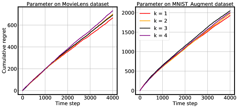
In this section, we conduct our parameter study for the neighborhood parameter on the MovieLens data set and MNIST-Aug data set with augmented labels, and the results are presented in Figure 3. For the MovieLens data set, we can observe that setting would give the best result. Although increasing can enable the aggregation module to propagate the hidden representations for multiple hops, it can potentially fail to focus on local arm group neighbors with high correlations, which is comparable to the aforementioned ”over-smoothing” problem. In addition, since the arm group graph of MovieLens data set only has 19 nodes, would be enough. Meantime, setting also achieves the best performance on the MNIST data set. The reason can be that the -hop neighborhood of each sub-class can already include all the other sub-classes from the same digit with heavy edge weights within the neighborhood for arm group collaboration. Therefore, unless setting to considerably large values, the AGG-UCB can maintain robust performances, which reduces the workload for hyperparameter tuning.
7. Conclusion
In this paper, motivated by real applications where the arm group information is available, we propose a new graph-based model to characterize the relationship among arm groups. Base on this model, we propose a novel UCB-based algorithm named AGG-UCB, which uses GNN to exploit the arm group relationship and share the information across similar arm groups. Compared with existing methods, AGG-UCB provides a new way of collaborating multiple neural contextual bandit estimators for obtaining the rewards. In addition to the theoretical analysis of AGG-UCB, we empirically demonstrate its superiority on real data sets in comparison with state-of-the-art baselines.
Acknowledgements.
This work is supported by National Science Foundation under Award No. IIS-1947203, IIS-2117902, IIS-2137468, and IIS-2002540. The views and conclusions are those of the authors and should not be interpreted as representing the official policies of the funding agencies or the government.References
- (1)
- Abbasi-Yadkori et al. (2011) Yasin Abbasi-Yadkori, Dávid Pál, and Csaba Szepesvári. 2011. Improved algorithms for linear stochastic bandits. NeurIPS 24 (2011), 2312–2320.
- Allen-Zhu et al. (2019) Zeyuan Allen-Zhu, Yuanzhi Li, and Zhao Song. 2019. A convergence theory for deep learning via over-parameterization. In ICML. PMLR, 242–252.
- Auer et al. (2002) Peter Auer, Nicolo Cesa-Bianchi, and Paul Fischer. 2002. Finite-time analysis of the multiarmed bandit problem. Machine learning 47, 2-3 (2002), 235–256.
- Ban and He (2021a) Yikun Ban and Jingrui He. 2021a. Convolutional neural bandit: Provable algorithm for visual-aware advertising. arXiv preprint arXiv:2107.07438 (2021).
- Ban and He (2021b) Yikun Ban and Jingrui He. 2021b. Local clustering in contextual multi-armed bandits. In Proceedings of the Web Conference 2021. 2335–2346.
- Ban et al. (2021) Yikun Ban, Jingrui He, and Curtiss B Cook. 2021. Multi-facet Contextual Bandits: A Neural Network Perspective. arXiv preprint arXiv:2106.03039 (2021).
- Ban et al. (2022a) Yikun Ban, Yunzhe Qi, Tianxin Wei, and Jingrui He. 2022a. Neural Collaborative Filtering Bandits via Meta Learning. ArXiv abs/2201.13395 (2022).
- Ban et al. (2022b) Yikun Ban, Yuchen Yan, Arindam Banerjee, and Jingrui He. 2022b. EE-Net: Exploitation-Exploration Neural Networks in Contextual Bandits. In ICLR.
- Blanchard et al. (2011) Gilles Blanchard, Gyemin Lee, and Clayton Scott. 2011. Generalizing from several related classification tasks to a new unlabeled sample. In NeurIPS. 2178–2186.
- Chlebus (2009) Edward Chlebus. 2009. An approximate formula for a partial sum of the divergent p-series. Applied Mathematics Letters 22, 5 (2009), 732–737.
- Chu et al. (2011) Wei Chu, Lihong Li, Lev Reyzin, and Robert Schapire. 2011. Contextual bandits with linear payoff functions. In AISTATS. 208–214.
- Deshmukh et al. (2017) Aniket Anand Deshmukh, Urun Dogan, and Clay Scott. 2017. Multi-task learning for contextual bandits. In NeurIPS. 4848–4856.
- Du et al. (2019b) Simon Du, Jason Lee, Haochuan Li, Liwei Wang, and Xiyu Zhai. 2019b. Gradient descent finds global minima of deep neural networks. In ICML. PMLR, 1675–1685.
- Du et al. (2019a) Simon S Du, Kangcheng Hou, Barnabás Póczos, Ruslan Salakhutdinov, Ruosong Wang, and Keyulu Xu. 2019a. Graph neural tangent kernel: Fusing graph neural networks with graph kernels. arXiv preprint arXiv:1905.13192 (2019).
- Durand et al. (2018) Audrey Durand, Charis Achilleos, Demetris Iacovides, Katerina Strati, Georgios D Mitsis, and Joelle Pineau. 2018. Contextual bandits for adapting treatment in a mouse model of de novo carcinogenesis. In Machine learning for healthcare conference. PMLR, 67–82.
- Fu and He (2021a) Dongqi Fu and Jingrui He. 2021a. DPPIN: A biological repository of dynamic protein-protein interaction network data. arXiv preprint arXiv:2107.02168 (2021).
- Fu and He (2021b) Dongqi Fu and Jingrui He. 2021b. SDG: A Simplified and Dynamic Graph Neural Network. In SIGIR ’21. 2273–2277.
- Gentile et al. (2017) Claudio Gentile, Shuai Li, Purushottam Kar, Alexandros Karatzoglou, Giovanni Zappella, and Evans Etrue. 2017. On context-dependent clustering of bandits. In ICML. 1253–1262.
- Gentile et al. (2014) Claudio Gentile, Shuai Li, and Giovanni Zappella. 2014. Online clustering of bandits. In ICML. 757–765.
- Hamilton et al. (2017) William L Hamilton, Rex Ying, and Jure Leskovec. 2017. Inductive representation learning on large graphs. arXiv preprint arXiv:1706.02216 (2017).
- He et al. (2016) Kaiming He, Xiangyu Zhang, Shaoqing Ren, and Jian Sun. 2016. Deep residual learning for image recognition. In CVPR. 770–778.
- He et al. (2017) Xiangnan He, Lizi Liao, Hanwang Zhang, Liqiang Nie, Xia Hu, and Tat-Seng Chua. 2017. Neural collaborative filtering. In WWW. 173–182.
- Hoang et al. (2021) NT Hoang, Takanori Maehara, and Tsuyoshi Murata. 2021. Revisiting Graph Neural Networks: Graph Filtering Perspective. In 2020 25th International Conference on Pattern Recognition (ICPR). IEEE, 8376–8383.
- Jacot et al. (2018) Arthur Jacot, Franck Gabriel, and Clément Hongler. 2018. Neural tangent kernel: Convergence and generalization in neural networks. arXiv preprint arXiv:1806.07572 (2018).
- Kipf and Welling (2016) Thomas N Kipf and Max Welling. 2016. Semi-supervised classification with graph convolutional networks. arXiv preprint arXiv:1609.02907 (2016).
- Klicpera et al. (2018) Johannes Klicpera, Aleksandar Bojchevski, and Stephan Günnemann. 2018. Predict then propagate: Graph neural networks meet personalized pagerank. arXiv preprint arXiv:1810.05997 (2018).
- Krause and Ong (2011) Andreas Krause and Cheng Soon Ong. 2011. Contextual Gaussian Process Bandit Optimization.. In NeurIPS. 2447–2455.
- Li et al. (2010) Lihong Li, Wei Chu, John Langford, and Robert E Schapire. 2010. A contextual-bandit approach to personalized news article recommendation. In WWW. 661–670.
- Li et al. (2019) Shuai Li, Wei Chen, Shuai Li, and Kwong-Sak Leung. 2019. Improved Algorithm on Online Clustering of Bandits. In IJCAI. 2923–2929.
- Li et al. (2016) Shuai Li, Alexandros Karatzoglou, and Claudio Gentile. 2016. Collaborative filtering bandits. In SIGIR. 539–548.
- Sajeev et al. (2021) Sandra Sajeev, Jade Huang, Nikos Karampatziakis, Matthew Hall, Sebastian Kochman, and Weizhu Chen. 2021. Contextual Bandit Applications in a Customer Support Bot. In KDD ’21. 3522–3530.
- Shao et al. (2019) Xin Shao, Ning Lv, Jie Liao, Jinbo Long, Rui Xue, Ni Ai, Donghang Xu, and Xiaohui Fan. 2019. Copy number variation is highly correlated with differential gene expression: a pan-cancer study. BMC medical genetics 20, 1 (2019), 1–14.
- Upadhyay et al. (2020) Sohini Upadhyay, Mikhail Yurochkin, Mayank Agarwal, Yasaman Khazaeni, et al. 2020. Online Semi-Supervised Learning with Bandit Feedback. arXiv preprint arXiv:2010.12574 (2020).
- Valko et al. (2013) Michal Valko, Nathaniel Korda, Rémi Munos, Ilias Flaounas, and Nelo Cristianini. 2013. Finite-time analysis of kernelised contextual bandits. arXiv preprint arXiv:1309.6869 (2013).
- Vershynin (2010) Roman Vershynin. 2010. Introduction to the non-asymptotic analysis of random matrices. arXiv preprint arXiv:1011.3027 (2010).
- Villar et al. (2015) Sofía S Villar, Jack Bowden, and James Wason. 2015. Multi-armed bandit models for the optimal design of clinical trials: benefits and challenges. Statistical science: a review journal of the Institute of Mathematical Statistics 30, 2 (2015), 199.
- Wang et al. (2015) Weiran Wang, Raman Arora, Karen Livescu, and Jeff A Bilmes. 2015. Unsupervised learning of acoustic features via deep canonical correlation analysis. In 2015 IEEE ICASSP. IEEE.
- Wei et al. (2020) Tianxin Wei, Ziwei Wu, Ruirui Li, Ziniu Hu, Fuli Feng, Xiangnan He, Yizhou Sun, and Wei Wang. 2020. Fast adaptation for cold-start collaborative filtering with meta-learning. In ICDM. IEEE, 661–670.
- Wu et al. (2019a) Felix Wu, Amauri Souza, Tianyi Zhang, Christopher Fifty, Tao Yu, and Kilian Weinberger. 2019a. Simplifying graph convolutional networks. In ICML. PMLR, 6861–6871.
- Wu et al. (2016) Qingyun Wu, Huazheng Wang, Quanquan Gu, and Hongning Wang. 2016. Contextual bandits in a collaborative environment. In SIGIR. 529–538.
- Wu et al. (2019b) Qingyun Wu, Huazheng Wang, Yanen Li, and Hongning Wang. 2019b. Dynamic Ensemble of Contextual Bandits to Satisfy Users’ Changing Interests. In WWW. 2080–2090.
- Xu et al. (2018) Keyulu Xu, Chengtao Li, Yonglong Tian, Tomohiro Sonobe, Ken-ichi Kawarabayashi, and Stefanie Jegelka. 2018. Representation learning on graphs with jumping knowledge networks. In ICML. PMLR, 5453–5462.
- Xu et al. (2021) Keyulu Xu, Mozhi Zhang, Stefanie Jegelka, and Kenji Kawaguchi. 2021. Optimization of graph neural networks: Implicit acceleration by skip connections and more depth. In ICML. PMLR, 11592–11602.
- You et al. (2019) Jiaxuan You, Rex Ying, and Jure Leskovec. 2019. Position-aware graph neural networks. In ICML. PMLR, 7134–7143.
- Zhang et al. (2020) Weitong Zhang, Dongruo Zhou, Lihong Li, and Quanquan Gu. 2020. Neural thompson sampling. arXiv preprint arXiv:2010.00827 (2020).
- Zhou et al. (2020) Dongruo Zhou, Lihong Li, and Quanquan Gu. 2020. Neural Contextual Bandits with UCB-based Exploration. arXiv:1911.04462 [cs.LG]
- Zhou et al. (2021a) Yao Zhou, Haonan Wang, Jingrui He, and Haixun Wang. 2021a. From Intrinsic to Counterfactual: On the Explainability of Contextualized Recommender Systems. ArXiv (2021). arXiv:2110.14844
- Zhou et al. (2021b) Yao Zhou, Jianpeng Xu, Jun Wu, Zeinab Taghavi Nasrabadi, Evren Körpeoglu, Kannan Achan, and Jingrui He. 2021b. PURE: Positive-Unlabeled Recommendation with Generative Adversarial Network. In KDD ’21. 2409–2419.
Appendix A Lemmas for Intermediate Variables and Weight Matrices
Due to page limit, we will give the proof sketch for lemmas at the end of each corresponding appendix section. Recall that each input context is embedded to (represented by for brevity). Supposing belongs to the arm group , denote as the corresponding row in matrix based on index of group in (if group is the -th group in , then is the -th row in ). Similarly, we have and respectively. Given received contexts and rewards , the gradient w.r.t. weight matrix will be
where is the diagonal matrix whose entries are the elements from . The coefficient of the cost function is omitted for simplicity. Then, for , we have
where . . Given the same , we provide lemmas to bound the term of Eq. 9. For brevity, the subscript and notation are omitted below by default.
Lemma A.1.
Given the randomly initialized parameters , with the probability at least and constants , we have
Proof. Based on the properties of random Gaussian matrices (Vershynin, 2010; Du et al., 2019b; Ban and He, 2021a), with the probability of at least , we have
where with . Applying the analogous approach for the other randomly initialized matrices would give similar bounds. Regarding the nature of , we can easily have . Then,
due to the assumed -Lipschitz continuity. Denoting the concatenated input for reward estimation module as , we can easily derive that . Thus,
Following the same procedure recursively for other intermediate outputs and applying the union bound would complete the proof.
Lemma A.2.
After time steps, run GD for -iterations on the network with the received contexts and rewards. Suppose . With the probability of at least and , we have
where
Proof. We prove this Lemma following an induction-based procedure (Du et al., 2019b; Ban and He, 2021a). The hypothesis is , and let . According to Algorithm 2, we have for the -th iteration and ,
by Cauchy inequality. For , we have
while for , we have . Combining all the results above and based on Lemma 5.8, it means that for ,
where the last inequality is due to Lemma A.3. Then, since we have , it leads to
For the last layer , the conclusion can be verified through a similar procedure. Analogously, for , we have
which leads to
Since (Lemma 5.8) and with sufficiently large , combining all the results above would give the conclusion.
Lemma A.3.
After time steps, with the probability of at least and running GD of -iterations on the contexts and rewards, we have and . With , we have
Proof. Similar to the proof of Lemma A.2, we adopt an induction-based approach. For , we have
where the last two inequalities are derived by applying Lemma A.2 and the hypothesis. For the aggregation module output ,
Then, for the first layer , we have
Combining all the results, for , it has
which completes the proof.
Lemma A.4.
With initialized network parameters and the probability of at least , we have
and the norm of gradient difference
with .
Proof. First, for , we have
For , we can also derive similar results. For ,
Then, with , we have the norm of gradient difference
Here, for the difference of , we have
To continue the proof, we need to bound the term as
Since for we have
we can derive
with sufficiently large , and this bound also applies to . For
Therefore, we have
By following a similar approach as in Lemma A.3, we will have
Therefore, we will have
with sufficiently large . This bound can also be derived for with a similar procedure. For -th layer, we have
which completes the proof.
Lemma A.5.
With the probability of at least , we have the gradient for all the network as
Proof. First, for the gradient before GD, we have
Then, for the norm of gradients, , we have
Then, for the network gradient after GD, we have
Lemma A.6.
With the probability of at least , for the initialized parameter , we have
and for the network parameter after GD, , we have
Proof. For the sake of enumeration, we let and . Then, we can derive
On the other hand, for network parameter after GD, we can have
This completes the proof.
Proof sketch for Lemmas A.1-A.6. First we derive the conclusions in Lemma A.1 with the property of Gaussian matrices. Then, Lemmas A.2 and A.3 are proved through the induction after breaking the target into norms of individual terms (variables, weight matrices) and applying Lemma A.1. Finally, for Lemmas A.4-A.6, we also decompose targets into norms of individual terms. Then, applying Lemmas A.1-A.3 the to bound these terms (at random initialization / after GD) would give the result.
Appendix B Lemmas for Gradient Matrices
Inspired by (Zhou et al., 2020; Ban and He, 2021a) and with sufficiently large network width , the trained network parameter can be related to ridge regression estimator where the context is embedded by network gradients. With the received contexts and rewards up to time step , we have the estimated parameter as where We also define the gradient matrix w.r.t. the network parameters as
where the notation is omitted by default. Then, we use the following Lemma to bound the above matrices.
Lemma B.1.
After iterations, with the probability of at least , we have
Proof. For the gradient matrix after random initialization, we have
with the conclusion from Lemma A.5. Then,
For the third inequality in this Lemma, we have
based on Lemma A.6.
Analogous to (Ban and He, 2021a; Zhou et al., 2020), we define another auxiliary sequence to bound the parameter difference. With , we have .
Lemma B.2.
After iterations, with the probability of at least , we have
Proof. The proof is analogous to Lemma 10.2 in (Ban and He, 2021a) and Lemma C.4 in (Zhou et al., 2020). Switching to would give the result.
Then, we can have the following lemma to bridge the difference between the regression estimator and the network parameter .
Lemma B.3.
Proof. With an analogous approach from Lemma 6.2 in (Ban and He, 2021a), we can have
With Lemma B.1, we can bound them as
based on the conclusion from Lemma A.2. For , we have
with proper choice of and . It leads to
which by induction and , we have
Finally,
which completes the proof.
Lemma B.4.
Proof. For the gradient matrix of ridge regression, we have
with the results from Lemma A.5. Then,
The proof is then completed.
Proof sketch for Lemmas B.1-B.4. Analogous to lemmas in Section A, Lemma B.1 is proved by Lemmas A.5, A.6 by breaking the target into the product of norms. The proof of Lemma B.2 is analogous to Lemma 10.2 in (Ban and He, 2021a) and Lemma C.4 in (Zhou et al., 2020), then replacing with would give the result. Then, based on Lemma B.2 results, Lemma B.3 will be proved with after bounding by induction. Finally, Lemma B.4 is proved by decomposing the norm into sum of individual terms, and bounding these terms with bounds on gradients in Lemma A.5.
Appendix C Lemmas for Model Convergence
Lemma C.1.
After time steps, assume the model with width defined in Lemma 5.3 are trained with the -iterations GD on the past contexts and rewards. Then, there exists a constant , such that , for any :
where , and .
Proof. We prove this lemma following an analogous approach as Lemma B.6 in (Du et al., 2019b). Given , we denote , and , where . By the definition of , we have its element
With the notation and conclusion from Lemma A.2, we have
Meantime, A similar form can also be derived for .