Network Dynamics-Based Framework for Explaining Deep Neural Networks

Although deep neural networks (DNNs) have achieved remarkable success [1, 2], their theoretical foundations are still not fully understood. Several influential theories, such as the information bottleneck theory [3, 4, 5, 6] and the flat minima hypothesis [7, 8, 9, 10], have been developed to explain DNNs. However, due to their high level of abstraction, limited generality, and computational complexity, a more straightforward and intuitive approach is required to elucidate the underlying mechanisms of DNNs. Central questions include why DNNs outperform shallow networks, what role hidden layers play, whether an optimal network size exists, how to determine it, and how to effectively tune hyperparameters such as depth, width, learning rate, batch size, dropout rate, and weight initialization to optimize network performance.

A critical gap in existing studies is the lack of a theoretical foundation based on the fundamental properties of neurons and neural networks. First, there is no clear definition or metric to quantify and characterize the degree of nonlinearity in networks. Typically, linear and nonlinear networks are distinguished by the properties of their activation functions. It is well known that certain nonlinear learning models initially exhibit behavior similar to that of linear neural networks (LNNs) before displaying characteristics of nonlinear neural networks (NNNs)[11, 12]. Therefore, distinguishing linear from nonlinear networks based on their qualitative behavior, rather than simply on the linearity or nonlinearity of their activation functions, is essential. Second, analytical approaches based on the basic building blocks of neural networks remain underdeveloped. Previous studies often treat neural networks as unified entities, even though it is well known that linear summation and activation are the fundamental computational processes at the level of individual neurons. Third, the dynamic behavior of networks has not been fully incorporated into the mechanistic analysis of neural networks. A learning model is, after all, a dynamical map that transforms inputs to outputs. In particular, the layers of a DNN can be viewed as an iterative process of dynamical systems, suggesting that dynamical theories could be utilized to understand learning dynamics. Finally, it remains an open question whether approaches based on linear models or shallow networks can fully capture the intrinsic advantages of DNNs. Clarifying the last point is particularly important, as many theoretical studies simplify DNNs in their analysis, either by linearizing the models [13, 14, 15, 16] or focusing on shallow networks [17, 18, 12].

In this paper, we establish an analytical framework that differs from traditional paradigms for analyzing the learning dynamics of DNNs. This framework is based on two novel concepts. First, we categorize neurons into two modes: order-preserving mode (OPM) and non-order-preserving mode (NPM), depending on whether their transformations preserve the input order. As is well known in nonlinear dynamics theory, the behavior of a dynamical system requires processes of stretching and folding for essential nonlinear dynamical behavior to emerge, not just nonlinearity in the system’s equations. Here, the NPM corresponds to the folding action. The ratio of neurons in the two modes quantifies the nonlinearity of neural networks and determines the degree of nonlinearity within hidden layers. These two modes lead to different information extraction strategies and effects. Allocating the ratio of neurons between the two modes across hidden layers provides a degree of freedom to maximize information extraction from the input layer, leading to improved accuracy compared to shallow networks.

Secondly, we introduce the concept of attraction basins in both input and weight vector spaces, characterizing generalization ability and structural stability, respectively. The former is directly related to the test accuracy, while the latter serves as a straightforward metric for flat minima. Although a duality exists between sample variations and weight variations[19], we show that the correlation between the two attraction basins is not always positive. The balance between these two basins determines the optimal performance. The ratio of neurons in the two modes may influence the size of attraction basins.

Based on these concepts, we can explain how an appropriate choice of depth, width, batch size, learning rate, and dropout rate leads to optimal performance. In particular, we can show that DNNs often transition between these two modes during the learning process. Phenomena such as grokking and double descent are examples of this transition. Grokking refers to a sudden increase in test accuracy after a prolonged plateau, which often indicates a shift from memorization to generalization following extensive training [20, 21, 22, 23, 24]. Under special conditions, the test loss may increase around the grokking time point, a phenomenon referred to as double descent. These two phenomena have been active research topics in recent studies on machine learning mechanisms.

We use MNIST dataset [25], a standard classification task, to illustrate our approach. This dataset consists of 60,000 training samples and 10,000 test samples, each represented as a $28\times 28$ grayscale image. Extending this approach to other tasks is straightforward.

The paper is organized as follows: In the next section, we present the two modes and the two types of attraction basins. We also define a set of quantities to describe the distribution and evolution of neurons between the two modes across hidden layers. In Section III, we examine the learning dynamics of shallow models, illustrating the roles of the two modes and the transitions in learning dynamics. Section IV focuses on DNNs, demonstrating that DNNs can self-organize into a standard structure, where early layers exhibit more nonlinearity, while later layers behave more linearly. Accordingly, we propose criteria for layer pruning. Pruning is essential to reduce operational costs[26, 27, 28, 29, 30, 31]. However, our research suggests that layer pruning results from the redundancy of deep layers. If the DNN size is optimal, pruning becomes unnecessary. Through neuron mode and attraction basin analysis, we identify the optimal depth, width, batch size, learning rate, and dropout rate for DNNs in this section. We explain the grokking and double descent phenomena in Section V. Finally, in the final section, we conclude our study and discuss the implications of our work.

Models and Algorithm. To illustrate our framework, we consider the commonly used fully connected DNNs, which are described by the following equations:

Here, $x^{(l)}_{i_{l}}$ represents the output of the $i_{l}$-th neuron in the $l$-th layer, and $h^{(l)}_{i_{l}}$ denotes the local field of the same neuron. The weight $w^{(l)}_{i_{l}i_{l-1}}$ connects the $i_{l-1}$-th neuron in the $(l-1)$-th layer to the $i_{l}$-th neuron in the $l$-th layer. The function $f(\cdot)$ represents the neuron’s transfer function. The number of neurons in the $l$-th layer is denoted by $N_{l}$.

Our computations are carried out using PyTorch, a widely adopted deep learning framework known for its flexibility and extensive community support. To meet the computational demands of deep learning training, experiments are executed on an NVIDIA L40S GPU, ensuring efficient processing and acceleration.

Modes of Neurons. We adopt the following perspective on information encoding. In classification networks, information from all samples must be processed together, considering their interrelationships. During training, the network should learn not only to recognize an input but also to differentiate it from others. In other words, classification relies on the mutual information among all samples. Specifically, a weight vector $\mathbf{w}$ projects a sample vector $\mathbf{x}^{\mu}$ onto a local field $h(\mu)=\mathbf{w}\cdot\mathbf{x}^{\mu}$, which then serves as the input to a neuron. The sequence $h(\mu)$, where $\mu=1,2,\ldots,P$, represents the local fields of the neuron for all $P$ samples. The ordering of this sequence, along with the spatial intervals among the $h(\mu)$ values, encodes the relationships and mutual information of the samples as projected along this weight vector. Different neurons capture different aspects of information through different weight vectors. In this sense, the scenario in Fig. 1(a) is preferable to Fig. 1(b), as it allows exploration of all possible projection directions.

After projection, the neural activation function transforms the sequence into the neuron’s outputs, aiming to minimize the loss. Typically, the goal is to ensure that the corresponding neuron in the output layer is activated for each class. To achieve this, a single neuron or a group of neurons in the hidden layer should produce higher activations for samples belonging to a specific class. This can be achieved through two modes of operation: the OPM and the NPM.

1. The OPM preserves the order of the inputs, i.e., the order of the sequence $h(\mu)$, where $\mu=1,2,\ldots,P$. Fig. 1(c) provides an example of this mode, demonstrated with a linear activation function. Even for strongly nonlinear Tanh-type activation functions, the transformation remains effectively linear as long as the order is preserved.

2. The NPM alters the order of the inputs. This can occur through individual nonlinear neurons or through combinations of neurons, such as those with Tanh-type activation functions, as shown in Fig. 1(d). This mode enables the maximization of a local field at any position in the sequence, which is characteristic of inherently nonlinear operations.

Thus, we define the fundamental processing units capable of performing inherently linear or nonlinear transformations. However, these two modes result in different distributions of the weight vectors. Specifically, in the OPM, the weight vectors must align with specific orientations to push the local fields of desired samples to the sequence boundaries, thereby maximizing output activations, as depicted in Fig. 1(b). Such directional convergence may cause information loss by ignoring potential directions.

In contrast, the NPM does not require such convergence of weight vectors, allowing greater freedom in extracting information from a broader range of weight directions, as demonstrated in Fig. 1(a). Consequently, the NPM enables better information extraction. However, neurons in the NPM exhibit greater sensitivity to input variations, whereas OPM neurons display minimal sensitivity, as indicated by a zero second-order derivative.

An optimal learning model should therefore combine neurons operating in both modes. By leveraging the stability and minimal sensitivity of OPM neurons while utilizing the flexibility and information extraction capabilities of NPM neurons, the model can achieve superior performance in both accuracy and robustness. This balance is crucial for developing effective neural networks that can handle complex and diverse datasets.

Attraction Basins. Our second key tool is the concept of attraction basins. Attraction basins are a fundamental concept in nonlinear dynamical systems. The analysis of attraction basins has been used to analyze the dynamics of asymmetric Hopfield neural networks [32, 33, 34], where a sharp transition from a chaotic phase to a memory phase occurs as the attraction basins expand [33, 34]. By treating the layers of a DNN as an iterative process, we extend the concept of attraction basins to DNNs. Here, we define the attraction basin of a training sample within two vector spaces. The coordinated expansion of the two attraction basins leads to optimal network performance.

First, we introduce random perturbations to a training sample and check whether the learned model can correctly classify these variations into the same class as the original sample. By plotting the average accuracy of the perturbed training set as a function of noise amplitude, one can observe a transition from the noise-free accuracy to an accuracy level corresponding to random guessing. The noise amplitude at which this transition occurs defines a metric for the attraction basin in the input vector space. Specifically, we use the threshold at which the accuracy drops to 50% of the noise-free accuracy to quantify the size of the attraction basin. This measure directly reflects the model’s generalization ability to input variations.

Another way to define the attraction basin is by perturbing the network weights with noise and examining if a training sample remains correctly classified. This type of attraction basin quantifies the network’s structural stability and its robustness to weight variations. According to the flat minima hypothesis, the flatness of these minima is typically measured by the sensitivity of the loss function to weight deviations, which significantly increases computational complexity, particularly due to the need for Hessian-based calculations. Here, we directly investigate the impact of weight changes on accuracy, offering a simple and quantifiable characterization of flat minima. There are two ways to characterize the attraction basin in weight vector space: using either the absolute or relative magnitude of weight perturbations to determine the basin size. The attraction basin measured by absolute perturbations indicates the absolute basin size in the solution space. The basin measured by relative perturbations indicates the robustness of the solution and is thus adopted in the present paper. It is important to note that the distinction between these two approaches is crucial for examining the dual relationship between weight and sample variations[19].

Quantities for Characterizing the Neuron Modes and DNN Structure. In a DNN, samples are progressively mapped through layers, eventually achieving linear separability in the output layer. This principle underpins the core paradigm of DNN-based classification. To characterize the linear separability of sample vectors as they propagate through the network toward the output layer, we train a linear perceptron (LP) to replace the DNN subsection beginning at the $l$-th layer. Specifically, the LP is trained using the sample set $(\mathbf{x}^{(l)}(\mu),\mathbf{y}(\mu)),\mu=1,\dots,P$, where $\mathbf{x}^{(l)}(\mu)$ represents the output of the $l$-th layer for the $\mu$-th sample, and $\mathbf{y}(\mu)$ denotes the corresponding final-layer local fields. When the outputs of a hidden layer become sufficiently linearly separable, the LP can effectively perform the classification task, indicating that the subsequent layers of the DNN can be replaced by this linear perceptron. For simplicity, we construct the LP based on least squares optimization. Such an LP-based approach has been previously employed in related studies[35, 36, 37, 38].

To evaluate the degree of linearity in the DNN starting from the $l$-th layer, we introduce a linear map (L-map) by replacing the nonlinear activation function $f(h)$ beyond this layer with a linear function $f(h)=h$. The L-map, characterized by the weight matrix

can effectively replace the subsequent layers of the network if the network behaves in a purely linear manner. Here, $\mathbf{W}^{(j)}$ denotes the weight matrix of the $j$-th layer. When the later section of a DNN is composed entirely of OPM neurons, the L-map functions as a linear perceptron without requiring additional training. Its purpose is to characterize the inherent linear structure of the DNN.

We introduce the concept of Ranking Position Distribution (RPD) as a quantitative tool to characterize the proportion of OPM and NPM neurons. As illustrated in Fig. 1(d), the NPM typically requires the collaboration of multiple nonlinear neurons to function effectively. Determining whether a neuron operates in OPM or NPM mode cannot be solely based on the degree of nonlinearity of its activation function. We define the RPD based on linear neural networks (LNNs) and extend it to general DNNs. For an LNN, $h_{i_{l-1}}^{(l-1)}(\nu)W^{\text{L-map}}_{ki}$ characterizes the contribution of the $i_{l-1}$-th neuron in the $(l-1)$-th layer to the $k$-th neuron (representing the $k$-th class) in the output layer, when the $\nu$-th sample is input. We rank $h_{i_{l-1}}^{(l-1)}(\nu)W^{\text{L-map}}_{ki}$ within the sequence $h_{i_{l-1}}^{(l-1)}(\mu)W^{\text{L-map}}_{ki}$ for $\mu=1,2,\dots,P$ to obtain its rank. The LNN possesses only the OPM mode, which requires weight vectors to aggregate towards specific directions, maximizing $h_{i_{l-1}}^{(l-1)}(\nu)W^{\text{L-map}}_{ki}$ for a sufficient number of neurons. In this case, the order of $h_{i_{l-1}}^{(l-1)}(\nu)W^{\text{L-map}}_{ki}$ should be high, ideally ranked ahead of all other classes. To characterize this effect, we calculate the rank of each sample with respect to its target neuron and then determine the distribution of ranking positions across all neurons in the layer. If the training is driven by the OPM, a high probability density in the high-ranking region is expected.

In a DNN with nonlinear activation functions, the OPM can similarly lead to an RPD with a high probability density in the high-ranking region. The NPM, on the other hand, transforms the local field at any position in the input sequence to achieve the maximum output, making it unrelated to rank and preventing concentration in the higher-ranking region. Therefore, the steepness of the RPD can serve as a qualitative indicator of the proportions of OPM and NPM neurons in a deep layer. A steep gradient may suggest a higher proportion of OPM neurons, while a flatter gradient may indicate a higher proportion of NPM neurons. Thus, we use the gradient of the RPD to quantitatively measure these proportions.

In this section, we demonstrate how to apply the quantities introduced in the previous section to analyze a shallow neural network (784-2048-10) designed for handwritten digit recognition using the MNIST dataset. Fig. 2(a) illustrates the network’s accuracy as a function of sample size. The accuracy of the NNN with Tanh activation, the LNN with linear activation, and the LP and L-map derived from the NNN are also presented. The LP is trained using the sample vectors as input and the network’s local field $h^{L}(\mu)$ as output.

For small training sets, we observe that the accuracy curves of all four models converge, indicating that the NNN behaves similarly to the LNN. Fig. 2(c) presents the RPDs of the hidden layer for both the Tanh-NNN and LNN, trained with 600 samples. In this shallow network, $h_{i_{2}}^{(2)}(\mu)W^{\text{L-map}}_{ki}=h_{i_{2}}^{(2)}(\mu)W^{(2)}_{ki_{2}}$, demonstrating the accuracy of the L-map approach. The RPDs exhibit a high probability density in the high-ranking region and a low probability density in the low-ranking region, suggesting that OPM neurons dominate the learning process. The close alignment of the RPD curves for the LNN and Tanh-NNN, along with the consistency with the LP and L-map methods, confirms that the NNN consists almost entirely of OPM neurons, with minimal activation of NPM neurons. This validates that the RPD effectively measures the degree of linearity of the NNN.

As the training set size increases, the accuracy curves begin to diverge, signaling the activation of NPM neurons. The degree of separation between the Tanh-NNN and L-map curves quantifies the accuracy loss induced by the linearization of the NNN with $f(h)=h$. Fig. 2(d) shows that the two RPDs diverge significantly at a training set size of 60,000, with the LNN exhibiting a steeper gradient. This confirms that a substantial number of NPM neurons are activated in the NNN.

The linearity of the NNN evolves throughout the training process. Fig. 2(b) illustrates accuracy as a function of training time using the 60,000-sample training set. Initially, the accuracy curves for all four models overlap but gradually diverge as training progresses. Fig. 2(e) shows the evolution of the RPD for the Tanh-NNN: the gradient initially increases, peaks, and then decreases as training nears completion. This pattern reflects that, in the early stages of training, learning is primarily driven by OPM neurons, as evidenced by the consistency of the accuracy curves. During this phase, weight vectors align towards specific directions, leading to an increase in the RPD gradient. As training progresses, NPM neurons become activated, causing the weight vectors to spread across broader directions, which in turn reduces the RPD gradient. This behavior is consistently observed for larger training sets. However, for small training sets that are well-linearly separable, the network may achieve its training objective during the OPM phase, thereby preserving its linear structure.

The Standard Structure of DNNs. In this section, we adopt the ReLU activation function for the NNNs and utilize all 60,000 MNIST training samples. We begin by training a DNN with 23 layers, each consisting of 1024 neurons, achieving a test accuracy of 98.6%. Fig. 3(a) examines the accuracy when applying LP pruning (replacing later layers with the LP) and L-map pruning (replacing later layers with the L-map) from the $l$-th hidden layer to the last. These results show that LP enables pruning at earlier layers, suggesting that samples become linearly separable after just a few layers. In contrast, L-map pruning can only be effectively applied in deeper layers, indicating that the final sections of the DNN transform into a pure LNN, functionally equivalent to a linear perceptron. This hierarchical structure, where earlier layers exhibit nonlinearity while later layers become linear, is commonly observed in DNNs using tanh-like activation functions, provided that the network depth and width remain within a moderate range. We refer to this as the ’standard structure’ of a DNN.

Fig. 3(b) presents the RPDs for several representative layers of the DNN. We observe that the RPD gradient increases with layer depth, indicating a decreasing proportion of NPM neurons as depth increases. When L-map pruning becomes effective, the RPD gradient reaches its maximum, confirming that the deeper layers of the network transition into a linear structure. We hypothesize that the high proportion of NPM neurons in the first layer, characterized by small RPD gradients, plays a key role in maximizing information extraction—a point we will revisit throughout this work.

Fig. 3(c) shows the evolution of the average cosine distance between a sample vector $\mathbf{x}^{(}l)(\mu)$ and the center vector of its class in the $l$-th layer as a function of network depth. For clarity, we plot the results for the first 100 samples from the digit "5" class. Additionally, we present the average cosine similarity between the center vectors of different classes.

We observe that, in general, as depth increases, samples tend to cluster around their class centers, while the center vectors of different classes become increasingly orthogonal. This progression demonstrates that the network effectively organizes the representation space, enhancing class separability with increasing depth. This advantage of DNNs has been previously documented.

Fig. 3(d) illustrates the test loss, test accuracy, and training accuracy as functions of training time for three DNNs with different depths. The grokking and double descent phenomena are evident and become more pronounced as the number of hidden layers increases. Before grokking, accuracy remains at the random guessing level, while the loss remains nearly unchanged. For deeper networks, the test loss may increase further just before grokking occurs, leading to the double descent phenomenon. We will revisit the mechanisms behind grokking and double descent in Section VI.

The Depth and Width Dependence. Fig. 4(a) shows the test accuracy as a function of depth for DNNs with widths ranging from 128 to 1280. We observe that, for a fixed width (except for the 128-width DNNs), the accuracy initially increases and then decreases as depth increases. This decrease is more pronounced in narrower networks, whereas wider networks exhibit a more gradual decline. The maximum accuracy is attained by DNNs with approximately 6 to 8 layers, and this result is roughly independent of width. For a fixed depth, accuracy generally increases with width and eventually saturates.

Fig. 4(b) depicts the gradient of RPDs for the first hidden layer of DNNs, illustrating how it varies with depth for different widths. Here, the RPD appears coarse due to the presence of NPM neurons in later layers, causing the L-map to provide only an approximate representation of the DNN’s contributions. Despite this, we observe a strong qualitative correspondence with Fig. 4(a). Specifically, a minimum RPD gradient occurs in DNNs with approximately 6 layers, indicating that this depth maximizes the proportion of NPM neurons in the first layer, thereby facilitating information extraction from the inputs. As width increases, the RPD gradient decreases and eventually saturates.

As mentioned earlier, NPM neurons extract information from broader directions in the input space. Fig. 4(b) provides an explanation for the observed depth and width dependence of accuracy in Fig. 4(a), viewed through the lens of information extraction. The decreasing RPD gradient with increasing width suggests that wider networks incorporate more NPM neurons, thereby improving test accuracy. The existence of a minimum in the gradient further reinforces the necessity of depth. That is, depth provides the flexibility to maximize information extraction by increasing the ratio of NPM neurons in the first layer.

Fig. 4(c) shows that increasing depth enlarges the attraction basin in the input vector space, suggesting that depth enhances generalization ability. This explains the origin of depth dynamics: layer-by-layer iteration progressively expands the attraction basin. However, its size saturates at approximately 8 layers. Comparing this with the results from Fig. 3(a), we infer that this saturation occurs because the deeper layers of the DNN transition into linear layers.

Fig. 4(d) shows that increasing depth reduces the attraction basin in the weight vector space, suggesting that deeper networks negatively impact structural stability. However, due to the formation of the ’standard structure,’ the attraction basin in the weight vector space eventually saturates, preventing further deterioration of structural stability.

To provide a comprehensive view of the dependence on both width and depth, we compute the size of the attraction basin for networks with varying depths as a function of width. Fig. 4(e) illustrates the attraction basin size in the input vector space. For a fixed depth, the attraction basin initially increases with width and eventually saturates. The rapid increase at smaller widths is attributed to the width approaching the effective dimensionality of the sample vectors, which in turn expands the information extraction space. This effect is also reflected in the proportion of neurons in the two modes, as shown in Fig. 4(b). As width increases, the RPD gradient decreases, leading to a higher proportion of NPM neurons.

Fig. 4(f) shows that increasing depth decreases the attraction basin in the input vector space, consistent with the results in Fig. 4(d). As width increases, the basin expands but eventually saturates. This provides structural stability support for the observation that increasing width improves accuracy.

Thus, while increasing depth enlarges the attraction basin in the input space, enhancing generalization capability, it also reduces stability in the weight vector space. Consequently, an optimal depth exists for a DNN. Fig. 4 suggests that this optimal depth lies around 6 to 8 layers, where the proportion of NPM neurons reaches a higher value (Fig. 4(b)), maximizing information extraction and achieving optimal test accuracy. Around the 8-layer index, the latter layers in deeper DNNs transition into linear layers (Fig. 3). Therefore, a 6–to–8-layer DNN appears to be an optimal choice for the original MNIST dataset.

The Role of weight initialization, batch size, dropout rate, and learning rate. In fact, the increase in the attraction basin in the weight vector space observed in Fig. 4(f) results from the default weight initialization strategy. In standard deep learning algorithms, frameworks such as PyTorch typically employ Kaiming initialization, which scales the initial weight magnitudes inversely with network width. If this initialization strategy is replaced with a fixed distribution range for the initial weights, Fig. 5(a) shows that when the width becomes inappropriate, the attraction basin in the weight space no longer expands and instead begins to shrink.

Other techniques, such as adjusting batch size, dropout rate, and learning rate, can also be interpreted as efforts to simultaneously maximize both attraction basins. In Figs. 5(b)-5(d), we plot the attraction basin size in both the input and weight vector spaces as functions of batch size, dropout rate, and learning rate for DNNs with 12 layers and a width of 1024. Test accuracy is also shown as a reference. Unless otherwise specified, we use the Adam algorithm with its default initial learning rate of 0.001. To obtain the results in Fig. 5(d), the SGD algorithm is used to study learning rate dependence, as the Adam algorithm automatically adjusts the learning rate during training. All results indicate that the maximum accuracy appears in the region where both types of attraction basins grow synchronously.

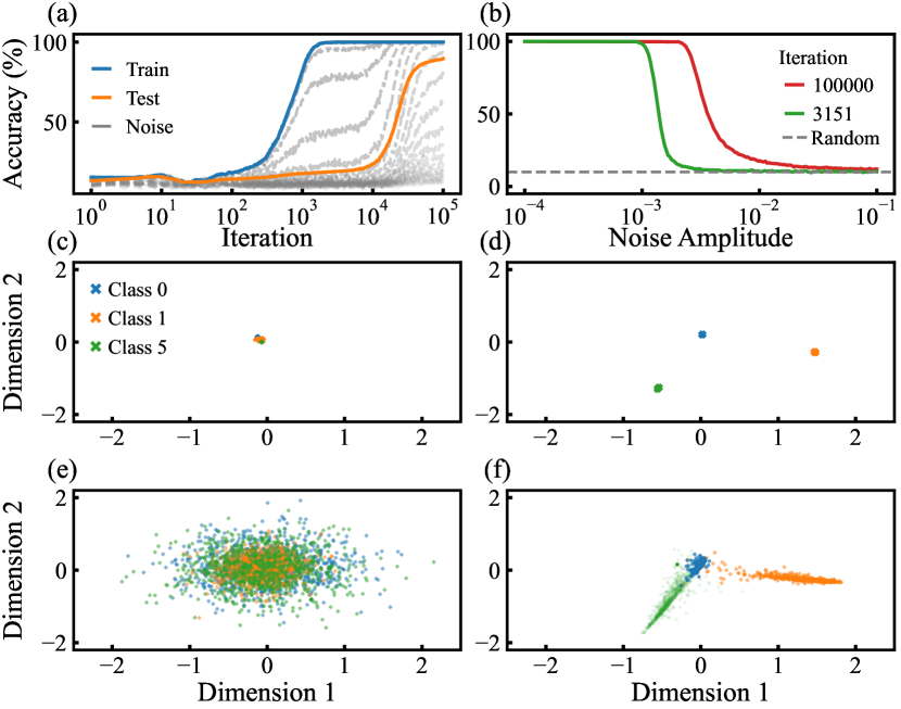
Grokking typically manifests as a sudden jump in test accuracy and test loss, indicating a sharp transition in the network’s dynamics. We first illustrate this transition in shallow networks that exhibit the grokking effect. To this end, we study a 784-200-200-10 network, which demonstrates a pronounced grokking phenomenon [39]. In Fig. 6(a), we reproduce the grokking phenomenon, showing a notable delay in test accuracy relative to training accuracy. The accuracy of noised training samples with different noise amplitudes is also presented. As the noise amplitude increases, we observe a clear transition. In Fig. 6(b), we plot the accuracy of noised training samples before and after grokking. The transition from near-perfect accuracy to random guessing accuracy occurs around $10^{-3}$, with the attraction basin expanding after grokking.

The grokking effect can be explained by the expansion of the attraction basin. Initially, the attraction basins of training samples are not fully established, causing both training and test accuracies to remain at random guessing levels. As training progresses, the basins expand, leading to increased training accuracy. However, due to their initially limited size, test samples may still fall outside these basins, maintaining random guessing accuracy. As the basins continue to expand, more test samples fall within them, resulting in increased test accuracy.

However, this scenario cannot fully explain the abrupt nature of grokking and why grokking does not always occur. To investigate this, we projected the sample representations onto two dimensions as follows. We added a bottleneck layer with two neurons before the output layer. Instead of retraining, we performed a singular value decomposition on the weight matrix of the original network’s final layer and extracted the two leading principal directions from $U,\Sigma,V^{T}$. Using these principal directions, we reconstructed the bottleneck layer’s weights. The local fields $h_{1}$ and $h_{2}$ of the two bottleneck neurons serve as the coordinates of the two-dimensional representation. We then plotted the projections of training samples (Figs. 6(c) and 6(d)) and test samples (Figs. 6(e) and 6(f)) for digits ’0,’ ’1,’ and ’5’ before and after grokking.

Before grokking, the projections of training samples are closely packed, whereas after grokking, they become well-separated. It can be verified that this separation is a sudden process accompanying grokking. Correspondingly, the projections of test samples are initially mixed and dispersed, indicating that they have not yet fallen within the attraction basins. After grokking, the projections of test samples align with those of the training samples, suggesting that they have entered the attraction basin. These observations indicate a transition in network dynamics, reminiscent of the behavior observed in asymmetric Hopfield networks [32], where a sharp transition from a chaotic phase to a memory phase occurs as the attraction basins expand [33, 34].

Nevertheless, this does not fully explain the mechanism of grokking in deep networks. As shown in Fig. 4(c), the attraction basin of a deep DNN is significantly larger than that of shallow networks. Once these basins are established, test samples with noise amplitudes up to $10^{-2}$ an still fall within the attraction basin. Moreover, the transition from near-perfect accuracy to random guessing accuracy occurs more gradually and is less abrupt. Consequently, grokking should not be observable under these conditions

The behavior observed in Fig. 3 is closely linked to the training algorithm used in DNNs, particularly batch normalization [40]. Batch normalization operates differently in training and evaluation modes [41]. During training, it normalizes each layer using the mean and variance computed from the current mini-batch. In evaluation mode, it instead applies a moving average of the mean and variance accumulated throughout training. The updates follow the formulas:

where $\hat{\mu}_{t}$ and $\hat{\sigma}^{2}_{t}$ are the moving average estimates used to normalize the test set, and $\mu_{t}$ and $\sigma_{t}^{2}$ are the current batch’s mean and variance, with $\alpha\approx 0.9$. This introduces a significant perturbation.

We demonstrate that the grokking effect observed in Fig. 3(d) is induced by the evaluation mode. In this mode, we plot the two-dimensional projections of training and test samples before and after grokking (Figs. 7(a) and 7(c) vs. 7(b) and 7(d)), obtained using the approach described earlier. Before grokking, the projections of test samples lie outside the attraction basin of training samples. After grokking, the test samples fall within the basin, leading to a sharp increase in test accuracy.

When we replace the evaluation mode with the training mode during the test phase (i.e., by setting $\alpha=0$), the grokking effect disappears. Fig. 7(e) to 7(f) show that the projection regions of training and test samples always overlap, which prevents the occurrence of grokking.

Thus, the grokking effect can be attributed to the perturbation introduced by the evaluation mode of batch normalization, which initially misaligns the projections of test samples with the attraction basin of training samples. As training progresses, the projections of test samples gradually fall into the basin, leading to increased accuracy.

Nonetheless, the evaluation mode does not always induce grokking. Figs. 8(a) and 8(b) show that grokking occurs with a larger batch size but not with a smaller one. Similarly, a smaller learning rate induces grokking, whereas a larger learning rate does not (Figs. 8(c) and 8(d)). The insets display two-dimensional projections for the digit ’5’ before and after grokking. These results confirm that grokking occurs as test samples transition from outside to inside the attraction basin.

The emergence of grokking is driven by an internal dynamical transition from an OPM learning phase to a mixed OPM-NPM phase. In the OPM phase, weight vectors concentrate in specific directions. Once NPM modes activate, the weight vectors spread out into broader directions, triggering a transition in the learning process. The batch normalization (BN) operation introduces a bias, initially causing the projections of test samples to deviate from the attraction basin. As training progresses, the network reaches a steady state with a fixed proportion of OPM and NPM neurons, gradually resolving the misalignment.

The transition in learning dynamics also explains why the test loss remains nearly unchanged or even increases (double descent) before grokking. Since most test samples fall outside the attraction basins prior to grokking, the test loss remains close to the random guessing level. When the hidden layers initially evolve synchronously in the OPM mode, weight vectors may converge excessively in specific directions, leading to a higher test loss and thus exhibiting the double descent phenomenon. To illustrate this effect, Figs. 9(a) and 9(b) show the evolution of the RPD gradient for the 23-layer and 32-layer DNNs studied in Fig. 3(d). The former does not exhibit double descent, whereas the latter does. We observe that in the case of double descent, the transition point of the RPD gradient occurs almost simultaneously across layers. This suggests that, early in training, all layers synchronously activate OPM neurons for learning, which may cause the weight vectors to converge in specific directions, thereby increasing the test loss. To further confirm this phenomenon, we examine two additional DNNs: one without double descent and one exhibiting double descent. The same pattern appears in the evolution of the RPD gradient, as shown in Figs. 9(c) and 9(d).

We analyze machine learning dynamics from a dynamical perspective, providing a clear and intuitive framework for understanding the learning process. The concepts of neuron modes and attraction basins play a central role in this analysis.

OPM neurons preserve the order of inputs, while NPM neurons partially reverse it. These two neuron modes define the network’s linear and nonlinear operations, respectively. We used the RPD to quantify the proportion of OPM and NPM neurons in hidden layers and employed LP pruning to assess the linear separability of samples as the number of hidden layers increases. This approach allows us to evaluate how effectively the earlier layers transform the data for class separation. Additionally, L-map pruning was used to examine the role of linearity in deeper layers, specifically assessing the extent of linearity in those layers.

Attraction basins in the input vector space reflect the model’s ability to generalize to new samples, while those in the weight vector space characterize the structural stability of the learning model. The latter provides a direct and intuitive measure of the flatness of minima. Unlike the flatness of minima defined by the loss function, we define structural stability based on the sensitivity of parameters to accuracy. The simultaneous expansion of both attraction basins promotes superior generalization, reinforced by enhanced structural stability.

Our analysis reveals the advantage of deep networks from a dynamical perspective. Increasing depth expands the attraction basin in the input space, granting DNNs greater degrees of freedom for self-organization. This self-organization optimizes the balance between OPM and NPM neurons, thereby enhancing network performance. As training progresses, the first hidden layer tends to accommodate more NPM neurons, facilitating greater information extraction from the input samples.

However, increasing depth can also reduce the attraction basin in the weight vector space, thereby decreasing structural stability. For sufficiently deep DNNs, both attraction basins reach saturation once the network depth exceeds a certain threshold, and the network converges to a stable structure with nonlinear layers in the early part of the network and linear layers in the later part. The linear layers can be pruned, as they no longer have a significant impact on accuracy.

Increasing the network width can also shrink the attraction basin in the weight vector space if the weight norm is fixed. Therefore, the commonly used initialization strategy of reducing the weight norm as the width increases in DNN training can be understood as a mechanism to facilitate the synchronous growth of both attraction basins, thereby improving accuracy. Similarly, techniques such as using a small batch size, applying an appropriate dropout rate, and selecting a suitable learning rate all contribute to the synchronous expansion of both basins, ultimately optimizing network performance.

Our neuron mode analysis reveals that DNNs may undergo a transition in learning dynamics. With typical initial parameters, a DNN initially activates only OPM neurons for learning. For smaller, linearly separable datasets, OPM neurons may be sufficient. However, as the dataset size increases, the learning process requires the activation of NPM neurons alongside OPM neurons to achieve training objectives in the later stages. During this phase, the first layer exhibits the highest concentration of NPM neurons.

This internal dynamical transition helps explain both the grokking and double descent phenomena. In shallow networks, the expansion of the attraction basin leads to an abrupt transition, resembling a phase change from a ’chaotic’ phase to a ’memory’ phase. In deep networks, grokking is often triggered by the evaluation mode of Batch Normalization. OPM neurons promote weight vector aggregation during the early learning stage, while NPM neurons facilitate weight vector exploration in the later learning stage. The evaluation mode leverages early training data to estimate the mean and variance of each layer’s output for test samples in the later stages, introducing a bias that prevents test samples from entering the attraction basin in the earlier stages. As training progresses, the ratio of OPM to NPM neurons stabilizes, ultimately leading to the grokking phenomenon.

The RPD effectively captures the transition in learning dynamics. At the grokking point, the ratio of OPM to NPM neurons shifts, marking a transition from linear to nonlinear learning. This transition also provides insight into the double descent phenomenon observed in learning dynamics, as it results from the extreme activation of OPM neurons prior to grokking.

Finally, we emphasize that grokking and double descent are not prerequisites for high performance. Our results demonstrate that DNNs achieving the highest accuracy do so without undergoing grokking, instead relying on the activation of NPM neurons from the beginning. We conclude that the true advantage of DNNs lies in the presence of NPM neurons, and analyzing them solely through the lens of linear learning models or shallow networks overlooks these critical dynamics.

Statement of Author Contributions. Specifically, Y.C.L. was responsible for performing the calculations and preparing the figures presented in this paper. Y.Z. conducted an extensive literature review and provided valuable insights during the analysis and discussion stages. S.H.F. carried out the initial exploratory research. Lastly, H.Z. proposed the concept of classifying neuron modes and introduced the idea of utilizing the basin of attraction for analyzing deep mechanisms. Additionally, H.Z. wrote the manuscript.

References

- He and Tao [2021] F. He and D. Tao, Recent advances in deep learning theory (2021), arXiv:2012.10931 [cs.LG] .
- Suh and Cheng [2024] N. Suh and G. Cheng, A survey on statistical theory of deep learning: Approximation, training dynamics, and generative models (2024), arXiv:2401.07187 [stat.ML] .
- Tishby and Zaslavsky [2015] N. Tishby and N. Zaslavsky, in 2015 IEEE Information Theory Workshop (ITW) (2015) pp. 1–5.
- Alemi et al. [2017] A. A. Alemi, I. Fischer, J. V. Dillon, and K. Murphy, in International Conference on Learning Representations (2017).
- Shwartz-Ziv [2022] R. Shwartz-Ziv, Information flow in deep neural networks (2022), arXiv:2202.06749 [cs.LG] .
- Murphy and Bassett [2024] K. A. Murphy and D. S. Bassett, Phys. Rev. Lett. 132, 197201 (2024).
- Jastrzębski et al. [2017] S. Jastrzębski, Z. Kenton, D. Arpit, N. Ballas, A. Fischer, Y. Bengio, and A. Storkey, arXiv preprint arXiv:1711.04623 (2017).
- Ma and Ying [2021] C. Ma and L. Ying, in Advances in Neural Information Processing Systems, edited by A. Beygelzimer, Y. Dauphin, P. Liang, and J. W. Vaughan (2021).
- Feng and Tu [2021] Y. Feng and Y. Tu, Proceedings of the National Academy of Sciences 118, e2015617118 (2021), https://www.pnas.org/doi/pdf/10.1073/pnas.2015617118 .
- Yang et al. [2023] N. Yang, C. Tang, and Y. Tu, Phys. Rev. Lett. 130, 237101 (2023).
- Geiger et al. [2021] M. Geiger, L. Petrini, and M. Wyart, Physics Reports 924, 1 (2021), landscape and training regimes in deep learning.
- Xu and Ziyin [2024] Y. Xu and L. Ziyin, Three mechanisms of feature learning in the exact solution of a latent variable model (2024), arXiv:2401.07085 [cs.LG] .
- Jacot et al. [2018] A. Jacot, F. Gabriel, and C. Hongler, in Proceedings of the 32nd International Conference on Neural Information Processing Systems, NIPS’18 (Curran Associates Inc., Red Hook, NY, USA, 2018) p. 8580–8589.
- Arora et al. [2019] S. Arora, S. S. Du, W. Hu, Z. Li, R. Salakhutdinov, and R. Wang, On exact computation with an infinitely wide neural net, in Proceedings of the 33rd International Conference on Neural Information Processing Systems (Curran Associates Inc., Red Hook, NY, USA, 2019).
- Saxe et al. [2014] A. Saxe, J. McClelland, and S. Ganguli, in International Conference on Learning Represenatations 2014 (2014).
- Ji and Telgarsky [2019] Z. Ji and M. Telgarsky, in International Conference on Learning Representations (2019).
- Dandi et al. [2023] Y. Dandi, F. Krzakala, B. Loureiro, L. Pesce, and L. Stephan, How two-layer neural networks learn, one (giant) step at a time (2023), arXiv:2305.18270 [stat.ML] .
- Luo et al. [2021] T. Luo, Z.-Q. J. Xu, Z. Ma, and Y. Zhang, J. Mach. Learn. Res. 22 (2021).
- Feng and Tu [2023] Y. Feng and Y. Tu, The activity-weight duality in feed forward neural networks: The geometric determinants of generalization (2023), arXiv:2203.10736 [cs.LG] .
- Power et al. [2022] A. Power, Y. Burda, H. Edwards, I. Babuschkin, and V. Misra, Grokking: Generalization beyond overfitting on small algorithmic datasets (2022), arXiv:2201.02177 [cs.LG] .
- Belkin et al. [2019] M. Belkin, D. Hsu, S. Ma, and S. Mandal, Proceedings of the National Academy of Sciences 116, 15849 (2019), https://www.pnas.org/doi/pdf/10.1073/pnas.1903070116 .
- Kumar et al. [2024] T. Kumar, B. Bordelon, S. J. Gershman, and C. Pehlevan, in The Twelfth International Conference on Learning Representations (2024).
- Schaeffer et al. [2024] R. Schaeffer, Z. Robertson, A. Boopathy, M. Khona, K. Pistunova, J. W. Rocks, I. R. Fiete, A. Gromov, and S. Koyejo, in The Third Blogpost Track at ICLR 2024 (2024).
- Nakkiran et al. [2020] P. Nakkiran, G. Kaplun, Y. Bansal, T. Yang, B. Barak, and I. Sutskever, in International Conference on Learning Representations (2020).
- Deng [2012] L. Deng, IEEE Signal Processing Magazine 29, 141 (2012).
- LeCun et al. [1989] Y. LeCun, J. Denker, and S. Solla, in Advances in Neural Information Processing Systems, Vol. 2, edited by D. Touretzky (Morgan-Kaufmann, 1989).
- Dalvi et al. [2020] F. Dalvi, H. Sajjad, N. Durrani, and Y. Belinkov, in Proceedings of the 2020 Conference on Empirical Methods in Natural Language Processing (EMNLP), edited by B. Webber, T. Cohn, Y. He, and Y. Liu (Association for Computational Linguistics, Online, 2020) pp. 4908–4926.
- Vadera and Ameen [2022] S. Vadera and S. Ameen, IEEE Access 10, 63280 (2022).
- He et al. [2024] S. He, G. Sun, Z. Shen, and A. Li, What matters in transformers? not all attention is needed (2024), arXiv:2406.15786 [cs.LG] .
- Gromov et al. [2024] A. Gromov, K. Tirumala, H. Shapourian, P. Glorioso, and D. A. Roberts, The unreasonable ineffectiveness of the deeper layers (2024), arXiv:2403.17887 [cs.CL] .
- Men et al. [2024] X. Men, M. Xu, Q. Zhang, B. Wang, H. Lin, Y. Lu, X. Han, and W. Chen, Shortgpt: Layers in large language models are more redundant than you expect (2024), arXiv:2403.03853 [cs.CL] .
- Zhao [2004] H. Zhao, Phys. Rev. E 70, 066137 (2004).
- Zhou et al. [2009] Q. Zhou, T. Jin, and H. Zhao, Neural Computation 21, 2931 (2009).
- Jin and Zhao [2005] T. Jin and H. Zhao, Phys. Rev. E 72, 066111 (2005).
- Yom Din et al. [2024] A. Yom Din, T. Karidi, L. Choshen, and M. Geva, in Proceedings of the 2024 Joint International Conference on Computational Linguistics, Language Resources and Evaluation (LREC-COLING 2024), edited by N. Calzolari, M.-Y. Kan, V. Hoste, A. Lenci, S. Sakti, and N. Xue (ELRA and ICCL, Torino, Italia, 2024) pp. 9615–9625.
- Belrose et al. [2023] N. Belrose, Z. Furman, L. Smith, D. Halawi, I. Ostrovsky, L. McKinney, S. Biderman, and J. Steinhardt, Eliciting latent predictions from transformers with the tuned lens (2023), arXiv:2303.08112 [cs.LG] .
- Pal et al. [2023] K. Pal, J. Sun, A. Yuan, B. Wallace, and D. Bau, in Proceedings of the 27th Conference on Computational Natural Language Learning (CoNLL), edited by J. Jiang, D. Reitter, and S. Deng (Association for Computational Linguistics, Singapore, 2023) pp. 548–560.
- Seshadri [2024] A. D. Seshadri, in Findings of the Association for Computational Linguistics: EMNLP 2024, edited by Y. Al-Onaizan, M. Bansal, and Y.-N. Chen (Association for Computational Linguistics, Miami, Florida, USA, 2024) pp. 5187–5192.
- Liu et al. [2023] Z. Liu, E. J. Michaud, and M. Tegmark, Omnigrok: Grokking beyond algorithmic data (2023), arXiv:2210.01117 [cs.LG] .
- Ioffe and Szegedy [2015] S. Ioffe and C. Szegedy, in Proceedings of the 32nd International Conference on International Conference on Machine Learning - Volume 37, ICML’15 (JMLR.org, 2015) p. 448–456.
- Paszke et al. [2019] A. Paszke, S. Gross, F. Massa, A. Lerer, J. Bradbury, G. Chanan, T. Killeen, Z. Lin, N. Gimelshein, L. Antiga, A. Desmaison, A. Kopf, E. Yang, Z. DeVito, M. Raison, A. Tejani, S. Chilamkurthy, B. Steiner, L. Fang, J. Bai, and S. Chintala, in Advances in Neural Information Processing Systems, Vol. 32, edited by H. Wallach, H. Larochelle, A. Beygelzimer, F. d'Alché-Buc, E. Fox, and R. Garnett (Curran Associates, Inc., 2019).