NESTED BANDITS
Abstract.
In many online decision processes, the optimizing agent is called to choose between large numbers of alternatives with many inherent similarities; in turn, these similarities imply closely correlated losses that may confound standard discrete choice models and bandit algorithms. We study this question in the context of nested bandits, a class of adversarial multi-armed bandit problems where the learner seeks to minimize their regret in the presence of a large number of distinct alternatives with a hierarchy of embedded (non-combinatorial) similarities. In this setting, optimal algorithms based on the exponential weights blueprint (like Hedge, EXP3, and their variants) may incur significant regret because they tend to spend excessive amounts of time exploring irrelevant alternatives with similar, suboptimal costs. To account for this, we propose a nested exponential weights (NEW) algorithm that performs a layered exploration of the learner’s set of alternatives based on a nested, step-by-step selection method. In so doing, we obtain a series of tight bounds for the learner’s regret showing that online learning problems with a high degree of similarity between alternatives can be resolved efficiently, without a red bus / blue bus paradox occurring.
Key words and phrases:
Online learning; nested logit choice; similarity structures; multi-armed bandits.2020 Mathematics Subject Classification:
Primary 68Q32; secondary 91B06.1. Introduction
Consider the following discrete choice problem (known as the “red bus / blue bus paradox” in the context of transportation economics). A commuter has a choice between taking a car or bus to work: commuting by car takes on average half an hour modulo random fluctuations, whereas commuting by bus takes an hour, again modulo random fluctuations (it’s a long commute). Then, under the classical multinomial logit choice model for action selection [19, 20], the commuter’s odds for selecting a car over a bus would be . This indicates a very clear preference for taking a car to work and is commensurate with the fact that, on average, commuting by bus takes twice as long.
Consider now the same model but with a twist. The company operating the bus network purchases a fleet of new buses that are otherwise completely identical to the existing ones, except for their color: old buses are red, the new buses are blue. This change has absolutely no effect on the travel time of the bus; however, since the new set of alternatives presented to the commuter is , the odds of selecting a car over a bus (red or blue, it doesn’t matter) now drops to . Thus, by introducing an irrelevant feature (the color of the bus), the odds of selecting the alternative with the highest utility have dropped dramatically, to the extent that commuting by car is no longer the most probable outcome in this example.
Of course, the shift in choice probabilities may not always be that dramatic, but the point of this example is that the presence of an irrelevant alternative (the blue bus) would always induce such a shift – which is, of course, absurd. In fact, the red bus / blue bus paradox was originally proposed as a sharp criticism of the independence from irrelevant alternatives (IIA) axiom that underlies the multinomial logit choice model [19] and which makes it unsuitable for choice problems with inherent similarities between different alternatives. In turn, this has led to a vast corpus of literature in social choice and decision theory, with an extensive array of different axioms and models proposed to overcome the failures of the IIA assumption. For an introduction to the topic, we refer the reader to the masterful accounts of McFadden [20], Ben-Akiva & Lerman [6] and Anderson et al. [2].
Perhaps surprisingly, the implications of the red bus / blue bus paradox have not been explored in the context of online learning, despite the fact that similarities between alternatives are prevalent in the field’s application domains – for example, in recommender systems with categorized product recommendation catalogues, in the economics of transport and product differentiation, etc. What makes this gap particularly pronounced is the fact that logit choice underlies some of the most widely used algorithmic schemes for learning in multi-armed bandit problems – namely the exponential weights algorithm for exploration and exploitation (EXP3) [27, 18, 3] as well as its variants, Hedge [4], EXP3.P [5], EXP3-IX [16], EXP4 [5] / EXP4-IX [22], etc. Thus, given the vulnerability of logit choice to irrelevant alternatives, it stands to reason that said algorithms may be suboptimal when faced with a set of alternatives with many inherent similarities.
Our contributions.
Our paper examines this question in the context of repeated decision problems where a learner seeks to minimize their regret in the presence of a large number of distinct alternatives with a hierarchy of embedded (non-combinatorial) similarities. This similarity structure, which we formalize in Section 2, is defined in terms of a nested series of attributes – like “type” or “color” – and induces commensurate similarities to the losses of alternatives that lie in the same class (just as the red and blue buses have identical losses in the example described above).
Inspired by the nested logit choice model introduced by McFadden [20] to resolve the original red bus / blue bus paradox, we develop in Section 3 a nested exponential weights (NEW) algorithm for no-regret learning in decision problems of this type. Our main result is that the regret incurred by nested exponential weights (NEW) is bounded as , where is the total number of alternatives and is the “effective” number when taking similarities into account (for example, in the standard red bus / blue bus paradox, , cf. Section 4). The gap between nested and non-nested algorithms can be quantified by the problem’s price of affinity (PoAf), defined here as the ratio measuring the worst-case ratio between the regret guarantees of the NEW and EXP3 algorithms (the latter scaling as in the problem at hand).
In practical applications (such as the type of recommendation problems that arise in online advertising), can be exponential in the number of attributes, indicating that the NEW algorithm could lead to significant performance gains in this context. We verify that this is indeed the case in a range of synthetic experiments in Section 5.
Related Work.
The problem of exploiting the structure of the loss model and/or any side information available to the learner is a staple of the bandit literature. More precisely, in the setting of contextual bandits, the learner is assumed to observe some “context-based” information and tries to learn the “context to reward” mapping underlying the model in order to make better predictions. Bandit algorithms of this type – like EXP4 – are often studied as “expert” models [5, 10] or attempt to model the agent’s loss function with a semi-parametric contextual dependency in the stochastic setting to derive optimistic action selection rules [1]; for a survey, we refer the reader to [17] and references therein. While the nested bandit model we study assumes an additional layer of information relative to standard bandit models, there are no experts or a contextual mapping conditioning the action taken, so it is not comparable to the contextual setup.
The type of feedback we consider assumes that the learner observes the “intra-class” losses of their chosen alternative, similar to the semi-bandit in the study of combinatorial bandit algorithms [11, 14]. However, the similarity with combinatorial bandit models ends there: even though the categorization of alternatives gives rise to a tree structure with losses obtained at its leaves, there is no combinatorial structure defining these costs, and modeling this as a combinatorial bandit would lead to the same number of arms and ground elements, thus invalidating the concept.
Besides these major threads in the literature, [26] recently showed that the range of losses can be exploited with an additional free observation, while [12] improves the regret guarantees by using effective loss estimates. However, both works are susceptible to the advent of irrelevant alternatives and can incur significant regret when faced with such a problem. Finally, in the Lipschitz bandit setting, [13, 15] obtain order-optimal regret bounds by building a hierarchical covering model in the spirit of [9]; the correlations induced by a Lipschitz loss model cannot be compared to our model, so there is no overlap of techniques or results.
2. The model
We begin in this section by defining our general nested choice model. Because the technical details involved can become cumbersome at times, it will help to keep in mind the running example of a music catalogue where songs are classified by, say, genre (classical music, jazz, rock,…), artist (Rachmaninov, Miles Davis, Led Zeppelin,…), and album. This is a simple – but not simplistic – use case which requires the full capacity of our model, so we will use it as our “go-to” example throughout.
2.1. Attributes, classes, and the relations between them
Let be a set of alternatives (or atoms) indexed by . A similarity structure (or structure of attributes) on is defined as a tower of nested similarity partitions (or attributes) , , of with . As a result of this definition, each partition captures successively finer attributes of the elements of (in our music catalogue example, these attributes would correspond to genre, artist, album, etc.).111The trivial partitions and do not carry much information in themselves, but they are included for completeness and notational convenience later on. Accordingly, each constituent set of a partition will be referred to as a similarity class and we assume it collects all elements of that share the attribute defining : for example, a similarity class for the attribute “artist” might consist of all Beethoven symphonies, all songs by Led Zeppelin, etc.
Collectively, a structure of attributes will be represented by the disjoint union
| (1) |
of all class/attribute pairs of the form for . In a slight abuse of terminology (and when there is no danger of confusion), the pair will also be referred to as a “class”, and we will write and instead of and respectively. By contrast, when we need to clearly distinguish between a class and its underlying set, we will write for the set of atoms contained in and for the attached attribute label.
Remark 1.
The reason for including the attribute label in the definition of is that a set of alternatives may appear in different partitions of in a different context. For example, if “IV” is the only album by Led Zeppelin in the catalogue, the album’s track list represents both the set of “all songs in IV” as well as the set of “all Led Zeppelin songs”. However, the focal attribute in each case is different – “artist” in the former versus “album” in the latter – and this additional information would be lost in the non-discriminating union (unless, of course, the partitions happen to be mutually disjoint, in which case the distinction between “union” and “disjoint union” becomes set-theoretically superfluous). 
Moving forward, if a class contains the class for some , we will say that is a descendant of (resp. is an ancestor of ), and we will write “” (resp. “”).222More formally, we will write when and . The corresponding weak relation “” is defined in the standard way, i.e., allowing for the case which in turn implies that . As a special case of this relation, if and , we will say that is a child of (resp. is parent of ) and we will write “” (resp. “”). For completeness, we will also say that and are siblings if they are children of the same parent, and we will write in this case. Finally, when we wish to focus on descendants sharing a certain attribute, we will write “” as shorthand for the predicate “ and ”.
Building on this, a similarity structure on can also be represented graphically as a rooted directed tree – an arborescence – by connecting two classes with a directed edge whenever . By construction, the root of this tree is itself,333Stricto sensu, the root of the tree is , but since there is no danger of confusion, the attribute label “0” will be dropped. and the unique directed path from to any class will be referred to as the lineage of . For notational simplicity, we will not distinguish between and its graphical representation, and we will use the two interchangeably; for an illustration, see Fig. 1.
2.2. The loss model
Throughout what follows, we will consider loss models in which alternatives that share a common set of attributes incur similar costs, with the degree of similarity depending on the number of shared attributes. More precisely, given a similarity class , we will assume that all its immediate subclasses share the same base cost (determined by the parent class ) plus an idiosyncratic cost increment (which is specific to the child in question). Formally, starting with (for the root class ), this boils down to the recursive definition
| (2) |
which, when unrolled over the lineage of a target class , yields the expression
| (3) |
Thus, in particular, when , the cost assigned to an individual alternative will be given by
| (4) |
Finally, to quantify the “intra-class” variability of costs, we will assume throughout that the idiosyncratic cost increments within a given parent class are bounded as
| (5) |
This terminology is justified by the fact that, under the loss model (2), the costs to any two sibling classes (i.e., any two classes parented by ) differ by at most . Analogously, the costs to any two alternatives that share a set of common attributes will differ by at most .
Example 1.
To represent the original red bus / blue bus problem as an instance of the above framework, let be the partition of the set by type (“bus” or “car”), and let be the corresponding sub-partition by color (“red” or “blue” for elements of the class “bus”). The fact that color does not affect travel times may then be represented succinctly by taking (representing the fact that color does not affect travel times). 
Remark 2.
We make no distinction here between and , i.e., between an alternative of and the (unique) singleton class of containing it. This is done purely for reasons of notational convenience. 
2.3. Sequence of events
With all this in hand, we will consider a generic online decision process that unfolds over a set of alternatives endowed with a similarity structure as follows:
-
(1)
At each stage , the learner selects an alternative by selecting attributes from one-by-one.
-
(2)
Concurrently, nature sets the idiosyncratic, intra-class losses for each similarity class .
-
(3)
The learner incurs for each chosen class for a total cost of , and the process repeats.
To align our presentation with standard bandit models with losses in , we will assume throughout that for all , meaning in particular that the maximal cost incurred by any alternative is upper bounded by . Other than this normalization, the sequence of idiosyncratic loss vectors , , is assumed arbitrary and unknown to the learner as per the standard adversarial setting [10, 24].
To avoid deterministic strategies that could be exploited by an adversary, we will assume that the learner selects an alternative at time based on a mixed strategy , i.e., . The regret of a policy , , against a benchmark strategy is then defined as the cumulative difference between the player’s mean cost under and , that is
| (6) |
where denotes the vector of costs encountered by the learner at time , i.e., for all . This definition will be our main figure of merit in the sequel.
3. The nested exponential weights algorithm
Our goal in what follows will be to design a learning policy capable of exploiting the type of similarity structures introduced in the previous section. The main ingredients of our method are a nested attribute selection and cost estimation rule, which we describe in detail in Sections 3.1 and 3.2 respectively; the proposed nested exponential weights (NEW) algorithm is then developed and discussed in Section 3.3.
3.1. Probabilities, propensities, and nested logit choice
We begin by introducing the attribute selection scheme that forms the backbone of our proposed policy. Our guiding principle in this is the nested logit choice (NLC) rule of McFadden [20] which selects an alternative by traversing one attribute at a time and prescribing the corresponding conditional choice probabilities at each level of .
To set the stage for all this, if is a mixed strategy on we will write
| (7) | ||||
| for the probability of choosing under , and | ||||
| (8) | ||||
for the conditional probability of choosing a descendant of assuming that has already been selected under .444Note here that the joint probability of selecting both and under is simply whenever . Then the nested logit choice (NLC) rule proceeds as follows: first, it prescribes choice probabilities for all classes (i.e., the coarsest ones); subsequently, once a class has been selected, NLC prescribes the conditional choice probabilities for all children of and draws a class from based on . The process then continues downwards along until reaching the finest partition and selecting an atom .
This step-by-step selection process captures the “nested” part of the nested logit choice rule; the “logit” part refers to the way that the conditional probabilities (8) are actually prescribed given the agent’s predisposition towards each alternative . To make this precise, suppose that the learner associates to each element a propensity score indicating their tendency – or propensity – to select it. The associated propensity score of a similarity class , , is then defined inductively as
| (9) |
where is a tunable parameter that reflects the learner’s uncertainty level regarding the -th attribute of . In words, this means that the score of a class is the weighted softmax of the scores of its children; thus, starting with the individual alternatives of – that is, the leaves of – propensity scores are propagated backwards along , and this is repeated one attribute at a time until reaching the root of .
Remark 4.
We should also note that Eq. 9 assigns a propensity score to any similarity class . However, because the primitives of this assignment are the original scores assigned to each alternative , we will reserve the notation for the profile of propensity scores that comprises the basis of the recursive definition (9). 
With all this in hand, given a propensity score profile , the nested logit choice (NLC) rule is defined via the family of conditional selection probabilities
| (NLC) |
where:
-
(1)
and is a child / parent pair of similarity classes of .
-
(2)
is a nonincreasing sequence of uncertainty parameters (indicating a higher uncertainty level for coarser attributes; we discuss this later).
In more detail, the choice of an alternative under (NLC) proceeds as follows: given a propensity score for each , every similarity class is assigned a propensity score via the recursive softmax expression (9), and the same procedure is applied inductively up to the root of . Then, to select an alternative , the conditional logit choice rule (NLC) proceeds in a top-down manner, first by selecting a similarity class , then by selecting a child of , and so on until reaching a leaf of .
Equivalently, unrolling (NLC) over the lineage of a target class , we obtain the expression
| (10) |
for the total probability of selecting class under the propensity score profile . Clearly, (NLC) and (10) are mathematically equivalent, so we will refer to either one as the definition of the nested logit choice rule.
3.2. The nested importance weighted estimator
The second key ingredient of our method is how to estimate the costs of alternatives that were not chosen under (NLC). To that end, given a cost vector and a mixed strategy with full support, a standard way to do this is via the importance-weighted estimator [8, 17]
| (IWE) |
where is the (random) element of chosen under .
This estimator enjoys the following important properties:
-
\edefnit\selectfonta\edefnn)
It is non-negative.
-
\edefnit\selectfonta\edefnn)
It is unbiased, i.e.,
(11) -
\edefnit\selectfonta\edefnn)
Its importance-weighted mean square is bounded as
(12)
This trifecta of properties plays a key role in establishing the no-regret guarantees of the vanilla exponential weights algorithm [4, 18, 27]; at the same time however, (IWE) fails to take into account any side information provided by similarities between different elements of . This is perhaps most easily seen in the original red bus / blue bus paradox: if the commuter takes a red bus, the observed utility would be immediately translateable to the blue bus (and vice versa). However, (IWE) is treating the red and blue buses as unrelated, so is not updated under (IWE), even though by default.
To exploit this type of similarities, we introduce below a layered estimator that shadows the step-by-step selection process of (NLC). To define it, let be a mixed strategy on with full support, and assume that an element is selected progressively according to as in the case of (NLC):555To clarify, this process adheres to the “nested” part of (NLC); the conditional probabilities may of course differ. First, the learner chooses a similarity class with probability ; subsequently, conditioned on the choice of , a class is selected with probability , and the process repeats until reaching a leaf of (at which point the selection procedure terminates and returns ). Then, given a loss profile and a mixed strategy , the nested importance weighted estimator (NIWE) is defined for all as
| (NIWE) |
where the chain of categorical random variables is drawn according to as outlined above.666The indicator in (NIWE) is assumed to take precedence over , i.e., if for some .
This estimator will play a central part in our analysis, so some remarks are in order. First and foremost, the non-nested estimator (IWE) is recovered as a special case of (NIWE) when there are no similarity attributes on (i.e., ). Second, in a bona fide nested model, we should note that is -measurable but not -measurable: this property has no analogue in (IWE), and it is an intrinsic feature of the step-by-step selection process underlying (NIWE). Third, it is also important to note that (NIWE) concerns the idiosyncratic losses of each chosen class, not the base costs of each alternative . This distinction is again redundant in the non-nested case, but it leads to a distinct estimator for in nested environments, namely
| (13) |
In particular, in the red bus / blue bus paradox, this means that an observation for the class “bus” automatically updates both and , thus overcoming one of the main drawbacks of (IWE) when facing irrelevant alternatives.
To complete the comparison with the non-nested setting, we summarize below the most important properties of the layered estimator (NIWE):
Proposition 1.
Let be a similarity structure on . Then, given a mixed strategy and a vector of cost increments as per (5), the estimator (NIWE) satisfies the following:
-
(1)
It is unbiased:
(14) -
(2)
It enjoys the importance-weighted mean-square bound
(15)
Accordingly, the loss estimator (13) is itself unbiased and enjoys the bound
| (16) |
where is defined as
| (17) |
with denoting the number of classes of attribute , and
| (18) |
denoting the “root-mean-square” range of all classes in .
Of course, Proposition 1 yields the standard properties of (IWE) as a special case when (in which case there are no similarities to exploit between alternatives). To streamline our presentation, we prove this result in Appendix B.
3.3. The nested exponential weights algorithm
We are finally in a position to present the nested exponential weights (NEW) algorithm in detail. Building on the original exponential weights blueprint [18, 4, 27], the main steps of the NEW algorithm can be summed up as follows:
-
(1)
For each stage , the learner maintains and updates a propensity score profile .
-
(2)
The learner selects an action based on the nested logit choice rule where is the method’s learning rate and is given by (NLC).
-
(3)
The learner incurs for each class and constructs a model of the cost vector of stage via (NIWE).
-
(4)
The learner updates their propensity score profile based on and the process repeats.
For a presentation of the algorithm in pseudocode form, see Algorithm 1; the tuning of the method’s uncertainty parameters and the learning rate is discussed in the next section, where we undertake the analysis of the NEW algorithm.
4. Analysis and results
We are now in a position to state and discuss our main regret guarantees for the NEW algorithm. These are as follows:
Theorem 1.
Suppose that Algorithm 1 is run with a non-increasing learning rate and uncertainty parameters against a sequence of cost vectors , , as per (4). Then, for all , the learner enjoys the regret bound
| (19) |
with given by (17) and defined by setting in (9) and taking , i.e.,
| (20) |
In particular, if Algorithm 1 is run with and , we have
| (21) |
Theorem 1 is our main regret guarantee for NEW so, before discussing its proof (which we carry out in detail in Appendices A, B and C), some remarks are in order.
The first thing of note is the comparison to the corresponding bound for EXP3, namely
| (22) |
This shows that the guarantees of NEW and EXP3 differ by a factor of777Depending on the source, the bound (22) may differ up to a factor of , compare for example [24, Corollary 4.2] and [17, Theorem 11.2]. This factor is due to the fact that (22) is usually stated for a known horizon (which saves a factor of relative to anytime algorithms). Ceteris paribus, the bound (21) can be sharpened by the same factor, but we omit the details.
| (23) |
which, for reasons that become clear below, we call the price of affinity (PoAf).
Since the variabilities of the idiosyncratic losses within each attribute have been normalized to (recall the relevant discussion in Section 2.3), Hölder’s inequality trivially gives , no matter the underlying similarity structure. Of course, if there are no similarities to exploit (), we get , in which case the two bounds coincide ().
At the other extreme, suppose we have a red bus / blue bus type of problem with, say, similarity classes, alternatives per class, and a negligible intra-class loss differential (). In this case, EXP3 would have to wrestle with alternatives, while NEW would only need to discriminate between alternatives, leading to an improvement by a factor of in terms of regret guarantee. Thus, even though the red bus / blue bus paradox could entangle EXP3 and cause the algorithm to accrue significant regret over time, this is no longer the case under the NEW method; we also explore this issue numerically in Section 5.
As another example, suppose that each non-terminal class in has children and the variability of the idiosyncratic losses likewise scales down by a factor of per attribute. In this case, a straightforward calculation shows that scales as , so the gain in efficiency would be of the order of , i.e., polynomial in and exponential in . This gain in performance can become especially pronounced when there is a very large number of atlernatives organized in categories and subcategories of geometrically decreasing impact on the end cost of each alternative. We explore this issue in practical scenarios in Sections 5 and D.
Finally, we should also note that the parameters of NEW have been tuned so as to facilitate the comparison with EXP3. This tuning is calibrated for the case where is fully symmetric, i.e., all subcategories of a given attribute have the same number of children. Otherwise, in full generality, the tuning of the algorithm’s uncertainty levels would boil down to a transcedental equation involving the nested term of (19). This can be done efficiently offline via a line search, but since the result would be structure-dependent, we do not undertake this analysis here.
Proof outline of Theorem 1.
The detailed proof of Theorem 1 is quite lengthy, so we defer it to Appendices A, B and C and only sketch here the main ideas.
The first basic step is to derive a suitable “potential function” that can be used to track the evolution of the NEW policy relative to the benchmark . The main ingredient of this potential is the “nested” entropy function
| (24) |
where for all (with by convention).888In the non-nested case, (24) boils down to the standard (negative) entropy . However, the inverse problem of deriving the “correct” form of in a nested environment involves a technical leap of faith and a fair degree of trial-and-error. As we show in Proposition A.1 in Appendix A, the “tiers” of can be unrolled to give the “non-tiered” recursive representation
| (25) |
where denotes the “conditional” entropy of relative to class . Then, by means of this decomposition and a delicate backwards induction argument, we show in Proposition A.2 that \edefnit\selectfonta\edefnn) the recursively defined propensity score of can be expressed non-recursively as ; and \edefnit\selectfonta\edefnn) that the choice rule (NLC) can be expressed itself as
| (26) |
This representation of (NLC) provides the first building block of our proof because, by Danskin’s theorem [7], it allows us to rewrite Algorithm 1 in more concise form as
| (NEW) |
with given by (13) appplied to . Importantly, this shows that the NEW algorithm is an instance of the well-known “follow the regularized leader” (FTRL) algorithmic framework [25, 24]. Albeit interesting, this observation is not particularly helpful in itself because there is no universal, “regularizer-agnostic” analysis giving optimal (or near-optimal) regret rates for “follow the regularized leader” (FTRL) with bandit/partial information.999For the analysis of specific versions of FTRL with non-entropic regularizers, cf. [ABL11, ZS19] and references therein. Nonetheless, by adapting a series of techniques that are used in the analysis of FTRL algorithms, we show in Appendix C that the iterates of ( ‣ 4) satisfy the “energy inequality”
| (27) |
where is the nested importance weighted estimator (13) for the cost vector encountered , and we have set
| (28) |
and .
Then, by Proposition 1, we obtain:
Proposition 2.
The NEW algorithm enjoys the bound
| (29) |
Proposition 2 provides the first half of the bound (19), with the precise form of derived in Lemma C.1. The second half of (19) revolves around the term and boils down to estimating how propensity scores are back-propagated along . In particular, the main difficulty is to bound the difference in the propensity score of the root node of when the underlying score profile is incremented to for some .
A first bound that can be obtained by convex analysis arguments is ; however, because the increments of ( ‣ 4) are unbounded in norm, this global bound is far too lax for our puposes. A similar issue arises in the analysis of EXP3, and is circumvented by deriving a bound for the log-sum-exp function using the identity for and the fact that the estimator (IWE) is non-negative [17, 24, 10]. Extending this idea to nested environments is a very delicate affair, because each tier in introduces an additional layer of error propagation in the increments . However, by a series of inductive arguments that traverse both forward and backward, we are able to show the bound
| (30) |
which, after taking expecations and using the bounds of Proposition 1, finally yields the pseudo-regret bound (19).
5. Numerical experiments


In this section we present a series of numerical experiments designed to test the efficiency of our method compared to EXP3. We use a synthetic environment where we simulate nested similarity partitions with trees. While NEW exploits the similarity structure by making forward/backward passes through the associated tree with its logit choice rule (NLC), EXP3 is simply run over the leaves of the tree, i.e., . All experiment details (as well as additional results) are presented in Appendix D. For every setting, we report the results of our experiments by plotting the average regret of each algorithm for seeds of randomly drawn losses. The code to reproduce the experiments can be found at https://github.com/criteo-research/Nested-Exponential-Weights.
Benefits in the red bus/blue bus problem.
We consider here a variant of the red bus/blue bus problem with different buses (the original paradox has ). In this experiment (see illustration in Fig. 5, Appendix D.2) we allow each bus to have non-zero intrinsic losses and illustrate in Fig. 2 how both algorithms perform when grows. We observe there that for all configurations NEW achieves better regret than EXP3. While both methods achieve sublinear regret, EXP3 requires far more steps to identify the best alternative as grows and suffers overall from worse regret while NEW achieves similar regret and does not suffer as much from the number of irrelevant alternatives. We provide additional plots in Section D.2 which show that NEW performs consistently better than EXP3 when there exists a similarity structure allowing to efficiently update scores of classes that have very similar losses.
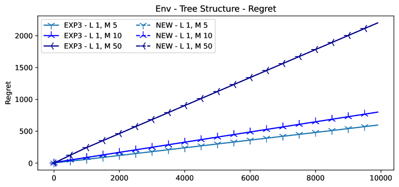
Performance in general nested structures.
In this setting we generate symmetric trees and experiment with different values of number of levels and number of child per nodes for . Specifically, in Fig. 3 with a fixed , we see that NEW obtains better regret than EXP3 even when increases. We provide variance plots for the experiments that generated the same performance on the plots in 8 as well as additional visualisations. Finally, in Fig. 4, we can see that for a shallow tree () NEW performs always better than EXP3, even for high values of . Indeed, when the number of children per nodes increases, the tree loses its “factorized” structure which also affects NEW due to the less "structured" tree. Thus, again, NEW performs consistently better than EXP3 when it is possible to efficiently handle classes with similar losses.
Overall, our experiments confirm that a learning algorithm based on nested logit choice can lead to significant benefits in problems with a high degree of similarity between alternatives. This leaves open the question of whether a similar approach can be applied to structures with non-nested attributes; we defer this question to future work.
Appendix A The nested entropy and its properties
Our aim in this appendix is to prove the basic properties of the series of (negative) entropy functions that fuel the regret analysis of the nested exponential weights (NEW) algorithm.
To begin with, given a similarity structure on and a sequence of uncertainty parameters (with by convention), we define:
-
(1)
The conditional entropy of relative to a target class :
(A.1) -
(2)
The nested entropy of relative to :
(A.2) where for all .
-
(3)
The restricted entropy of relative to :
(A.3) where denotes the (convex) characteristic function of , i.e., if and otherwise. [Obviously, whenever .]
Remark 1.
As per our standard conventions, we are treating interchangeably as a subset of or as an element of ; by analogy, to avoid notational inflation, we are also viewing as a subset of – more precisely, a face thereof. Finally, in all cases, the functions , and are assumed to take the value for . 
Remark 2.
For posterity, we also note that the nested and restricted entropy functions ( and respectively) are both convex – though not necessarily strictly convex – over . This is a consequence of the fact that each summand in (A.2) is convex in and that for all . Of course, any two distributions that assign the same probabilities to elements of but not otherwise have , so is not strictly convex over if . However, since the function is strictly convex over , it follows that – and hence – is strictly convex over . 
Our main goal in the sequel will be to prove the following fundamental properties of the entropy functions defined above:
Proposition A.1.
For all , , and for all , we have:
| (A.4) | ||||
| Consequently, for all , we have: | ||||
| (A.5) | ||||
Proposition A.2.
For all and all , we have:
-
(1)
The recursively defined propensity score of as given by (9) can be equivalently expressed as
(A.6) (A.7)
These propositions will be the linchpin of the analysis to follow, so some remarks are in order:
Remark 3.
Remark 4.
The first part of Proposition A.2 can be rephrased more concisely (but otherwise equivalently) as
| (A.8) |
where
| (A.9) |
denotes the convex conjugate of . This interpretation is conceptually important because it spells out the precise functional dependence between the (primitive) propensity score profile and the propensity scores that are propagated to higher-tier similarity classes via the recursive definition (9). In particular, this observation leads to the recursive rule
| (A.10) |
We will we use this representation freely in the sequel. 
Remark 5.
It is also worth noting that the propensity scores , , can also be seen as primitives for the arborescence obtained from by excising all (proper) descendants of . Under this interpretation, the second part of Proposition A.2 readily gives the more general expression
| (A.11) |
where, in the right-hand side, is to be construed as a function of , defined recursively via (9) applied to the truncated arborescence . Even though we will not need this specific result, it is instructive to keep it in mind for the sequel.
The rest of this appendix is devoted to the proofs of Propositions A.1 and A.2.
Proof of Proposition A.1.
Let , and fix some attribute label . We will proceed inductively by collecting all terms in (A.4) associated to the attribute and then summing everything together. Indeed, we have:
| # collect attributes | ||||
| # by definition | ||||
| (A.12a) | ||||
| (A.12b) | ||||
with the tacit understanding that any empty sum that appears above is taken equal to zero.
Now, by the definition of the nested entropy, we readily obtain that
| (A.13a) | |||
| whereas, by noting that (by the definition of conditional class choice probabilities), Eq. A.12b becomes | |||
| (A.13b) | |||
Hence, combining Eqs. A.12, A.13a and A.13b, we get:
| (A.14) |
The above expression is our basic inductive step. Indeed, summing (A.14) over all , we obtain:
| # by definition | ||||
| # isolate | ||||
| # by (A.14) | ||||
| (A.15) |
with the last equality following by telescoping the terms involving . Now, given that by convention, the third sum above is zero. Finally, since the conditional entropy of relative to any childless class is zero by definition, the first sum in (A.15) can be rewritten as , and our claim follows.
Finally, (A.5) is a consequence of the fact that whenever – i.e., whenever . ∎
Proof of Proposition A.2.
We begin by noting that the optimization problem (A.6) can be written more explicitly as
| maximize | () | |||
| subject to |
We will proceed to show that the (unique) solution of () is given by the vector of conditional probabilities . The expression (A.6) for the maximal value of () will then be derived from Proposition A.1, and the differential representation (A.7) will follow from Legendre’s identity. We make all this precise in a series of individual steps below.
Step 1: Optimality conditions for ().
For all , the definition of the nested entropy gives
| (A.16) |
where denotes the lineage of up to (inclusive). This implies that whenever , so any solution of () must have for all . In view of this, the first-order optimality conditions for () become
| (A.17) |
where is the Lagrange multiplier for the equality constraint .101010Since for all , the multipliers for the corresponding inequality constraints all vanish by complementary slackness. Thus, after rearranging terms and exponentiating, we get
| (A.18) |
for some proportionality constant .
Step 2: Solving ().
The next step of our proof will focus on unrolling the chain (A.18), one attribute at a time. To start, recall that , so (A.18) becomes
| (A.19) |
where we used the fact that by definition. Now, since , it follows that all children of are also desendants of , so (A.19) applies to all siblings of as well. Hence, summing (A.19) over , we get
| (A.20) |
where we used the definition (7) of and the recursive definition (9) for , i.e., the fact that . Therefore, noting that
| (A.21) |
the product (A.20) becomes
| (A.22) |
or, equivalently
| (A.23) |
This last equation has the same form as (A.20) applied to the chain instead of . Thus, proceeding inductively, we conclude that
| (A.24) |
with the empty product taken equal to by standard convention.
Now, substituting in (A.24), we readily get
| (A.25) |
Consequently, recalling that and dividing (A.24) by (A.25), we get
| (A.26) |
and hence
| (A.27) |
by the definition of the conditional logit choice model (NLC). Therefore, by unrolling the chain
| (A.28) |
we obtain the nested expression
| (A.29) |
Thus, with (by the fact that ), we finally conclude that
| (A.30) |
Step 3: The maximal value of ().
To obtain the value of the maximization problem (), we will proceed to substitute (A.30) in the expression (A.4) provided by Proposition A.1 for . To that end, for all and all , the definition (A.1) of the conditional entropy gives:
| # by definition | ||||
| # by (A.27) | ||||
| # since | ||||
| (A.31) |
and hence
| (A.32) |
Thus, telescoping this last releation over and invoking Proposition A.1, we obtain:
| # by Proposition A.1 | ||||
| # collect parent classes | ||||
| # by (A.32) | ||||
| (A.33) |
where, in the second line, we used the fact that the conditional entropy relative to any childless class is zero by definition. Accordingly, substituting back to () we conclude that
| (A.34) |
as claimed.
Step 4: Differential representation of conditional probabilities.
To prove the second part of the proposition, recall that the restricted entropy function is convex, and let
| (A.35) |
denote its convex conjugate.111111Note here that is bounded from above by the convex conjugate of because the latter does not include the constraint . By standard results in convex analysis [e.g., Theorem 23.5 in 23], is differentiable in and we have the Legendre identity:
| (A.36) |
Now, by (A.30), we have whenever solves () and hence, by Fermat’s rule, whenever . Our claim then follows by noting that and combining the first and third legs of the equivalence (A.36). ∎
These properties of the nested entropy function (and its restricted variant) will play a key role in deriving a suitable energy function for the nested exponential weights algorithm. We make this precise in Appendix C below.
Appendix B Auxiliary bounds and results
Throughout this appendix, we assume the following primitives:
-
•
A fixed sequence of real numbers ; all entropy-related objects will be defined relative to this sequence as per the previous section.
- •
-
•
A vector of cost increments that defines an associated cost vector as per (4), viz.
(B.1)
Moreover, for all , we define the nested power sum function which, to any , associates the real number
| (B.2) |
The following lemma links the increments of the conjugate entropy to the nested power sum defined above:
Lemma B.1.
For all , , we have
| (B.3) |
Lemma B.1 will be proved as a corollary of the more general result below:
Lemma B.2.
Fix some and . Then, for all , ,we have
| (B.4) |
Proof of Lemma B.2.
We proceed by descending induction on .
Base step.
Induction step.
Fix some with , , and suppose that (B.4) holds at level . We then have:
| # inductive hypothesis | ||||
| (B.6) |
with the last equality following from the definition of and . This being true for all with , the inductive step and – a fortiori – our proof are complete. ∎
The next lemma provides an upper bound for , which will in turn allow us to derive a bound for the increment of .
Lemma B.3.
For and , we have:
| (B.7) |
As in the case of B.1, Lemma B.3 will follow as a special case of the more general, class-based result below:
Lemma B.4.
Fix some and . Then, for all , ,we have
| (B.8) |
Proof of Lemma B.4.
We proceed again by descending induction on .
Base step.
Fix some with . We then have:
| # for | ||||
| (B.9) |
so the initialization of the induction process is complete.
Induction step.
Fix some with , , and suppose that (B.8) holds at level . We then have:
| # inductive hypothesis | ||||
| # for | ||||
| (B.10) | ||||
| (B.11) |
This being true for all s.t. , the induction step and the proof of our assertion are complete. ∎
With all this in hand, we are now in a position to upper bound the increments of the conjugate nested entropy .
Proposition B.1.
For and , we have:
| (B.12) |
Proof.
Using Lemmas B.1 and B.3 and the concavity inequality directly delivers our assertion. ∎
Remark 6.
It is useful to note that, given a cost increment vector with associated aggregate costs given by we have:
We are finally in a position to prove the basic properties of the nested importance weighted estimator (NIWE) estimator, which we restate below for convenience:
See 1
Proof.
Fix some with and lineage . We will now prove both properties of the (NIWE) estimator.
- Part 1.
-
Part 2.
We now turn to the proof of the importance-weighted mean-square bound of the estimator (NIWE). In this case, for any , we have:
# because (B.14)
We are left to derive the bound for the aggregate cost estimator (13), viz.
| (B.15) |
With this in mind, we can write:
| (B.16) |
Now, decomposing the above sums attribute-by-attribute and taking expectations in (B.16), we get:
| (B.17) |
The first term in (B.17) can simply be bounded using (B.14). Indeed:
| (B.18) |
with for any .
We now turn to the second term in (B.17). Let be any fixed sequence of positive numbers. For any and any and , the Peter-Paul inequality yields:
| (B.19) |
Appendix C Regret analysis
As we mentioned in the main text, the principal component of our analysis is a recursive inequality which, when telescoped over , will yield the desired regret bound. To establish this “template inequality”, we will first require an energy function measuring the disparity between a benchmark strategy and a propensity score profile . To that end, building on the notions introduced in Appendix A, let denote the total nested entropy function
| (C.1) | ||||||
| and let | ||||||
| (C.2) | ||||||
denote the convex conjugate of so, by Proposition A.2, we have
| (C.3) |
The Fenchel coupling between and is then defined as
| (C.4) |
and we have the following key result:
Proposition C.1.
Proof.
Our first claim follows by setting in Propositions A.1 and A.2 and noting that when : indeed, by Young’s inequality, we have with equality if and only if , so the equality follows from (A.36) applied to and the fact that . As for our second claim, simply note that and set in the definition (C.4) of the Fenchel coupling. ∎
With all this in hand, the specific energy function that we will use for our regret analysis is the “rate-deflated” Fenchel coupling
| (C.7) |
where is the regret comparator, is the algorithm’s learning rate at stage , and is the corrsponding propensity score estimate. In words, since the mixed strategy employed by the learner at stage is , the energy essentially measures the disparity between and the target strategy (suitably rescaled by the method’s learning rate). We then have the following fundamental estimate:
Proposition C.2.
For all and all , we have:
| (C.8) |
Proof.
By the definition of , we have
| (C.9a) | ||||
| (C.9b) | ||||
We now proceed to upper-bound each of the two terms (C.9a) and (C.9b) separately.
For the term (C.9a), the definition of the Fenchel coupling (C.4) readily yields:
| (C.10) |
Inspired by a trick of Nesterov [21], consider the function . Then, by Proposition A.2, letting and differentiating with respect to gives
| (C.11) |
Since , the above shows that . Accordingly, setting in the definition of yields
| (C.12) |
and hence
| (C.13) |
Now, after a straightforward rearrangement, the second term of (C.9) becomes
| # by ( ‣ 4) | ||||
| # isolate benchmark | ||||
| # by Proposition A.2 | ||||
| (C.14) |
We are now in a position to state and prove the template inequality that provides the scaffolding for our regret bounds:
See 2
Proof.
Let denote the error in the learner’s estimation of the -th stage payoff vector . Then, by substituting in Proposition C.2 and rearranging, we readily get:
| (C.16) |
Thus, telescoping over , we have
| (C.17) |
where we used the fact that \edefnit\selectfonta\edefnn) for all (a consequence of the first part of Proposition C.1); and that \edefnit\selectfonta\edefnn) (from the second part of the same proposition). Our claim then follows by taking expectations in (C) and noting that (by Proposition 1). ∎
In view of the above, our main regret bound follows by bounding the two terms in the template inequality (C.8). The second term is by far the most difficult one to bound, and is where Appendix B comes in; the first term is easier to handle, and it can be bounded as follows:
Lemma C.1.
Suppose that each class has at most children, . Then, for all we have
| with equality iff the tree is symmetric, | (C.18) | ||||
| (C.19) |
Proof.
Suppose that for all . Then, applying (9) inductively, we have:
| for all | (C.20) | |||||
| for all | ||||||
| for all | ||||||
| for all |
and hence . Eq. C.18 then follows from Proposition C.1.
Proposition C.3.
For all and all , we have:
| (C.22) |
Proof.
Let and , we simply write:
| # |
and our assertion follows. ∎
We are finally in a position to prove our main result (which we restate below for convenience):
See 1
Proof.
Injecting Eq. C.22 in the result of Proposition 2 and using Proposition B.1 and Eq. 16 of Proposition 1 directly yields the pseudo-regret bound (19).
Appendix D Additional Experiment Details and Discussions
In this appendix we provide additional details on the experiments as well as further discussions on the settings we presented. The code with the implementation of the algorithms as well as the code to reproduce the figures will be open-sourced and is provided along with the supplementary materials.
D.1. Experiment additional details
In the synthetic environment, at each level, the rewards are generated randomly according for each class nodes, through uniform distributions of randomly generated means and fixed bandwidth. From a level to the next , the rewards range are divided by a multiplicative factor . The implemented method of NEW uses the reward based IW. Moreover, no model selection was used in this experiment as no hyperparameter was tuned. Indeed, a decaying rate of was used for the score updates for all methods, as is common in the bandit litterature [17].
D.2. Blue Bus/ Red Bus environment
We detail in Figure 5 a graphical representation of such blue bus/red bus environment, where many colors of the bus item build irrelevant alternatives. In this setting, with few arms, we run the methods up to the horizon . We provide in Figure 6 the average reward of the two methods NEW and EXP3 with varying number of subclasses of the “bus”.
While the NEW method ends up selecting the best alternative and having the lowest regret, the EXP3 seems to pick wrong alternative in some experiments, and ends up having higher regret and requiring more iterations to converge to higher average reward. In some of our experiments over the multiple random runs, alternatives of very low sampling probability that were sampled changed the score vector too brutally in the IPS estimator which seemed to hurt the EXP3 method much more than the NEW algorithm.


D.3. Tree structures
In this appendix we show additional results and visualisations for the second setting presented in the main paper. We start with discussions on the depth parameter and follow with the breadth parameter related to the number of child per class .
Influence of the depth parameter
In Figure 7 we show the influence of the depth parameter with a fixed number of child per class. By making the tree deeper, we illustrate the effect of knowing the nested structure compared to running the logit choice to the whole alternative set. As shown in both the regret and average reward plots, the NEW method outperforms the EXP3 algorithm. While the NEW method also use an IPS estimator, it is less prone to variance issues than the EXP3 method. Indeed, due to the nested structure and the reward decay related to the ratio , the NEW estimator end up not hurting the regret by still selecting "right" parent classes.


Influence of the number of child per class (wideness)
In this setting we fix the number of levels and vary the number of child per classes . In Figure 8 we can see that the NEW method outperforms the EXP3 in terms of regret and average reward. Interestingly, we see that the gap between the two methods shrinks when the number of child per class augments. This is because when the size of a class increase, the NEW method also end up having less knowledge locally and end up having a large number of alternatives to choose among.


D.4. A visualisation of the effects of NEW
In this appendix we want to show the effects of NEW through the simple setting where we assume a nested structure with and . We illustrate in Figure 9 the score vectors of the NEW method along the optimal path in the tree (path which nodes have the highest cumulated mean, i.e which generates the highest reward) along with the oracle means of the child nodes. We can see that the algorithm takes advantage of the nested structure and updates the scores vectors optimally with regards to the oracle means of all the nodes. The NEW algorithm therefore estimates correctly the rewards of the environment.


Inversely we see in Figure 10 that the EXP3 method has suffered from variance issue and selected a suboptimal alternative among the possible ones. The EXP3 did not take advantage of the nested structure and therefore did not learn as correctly as the NEW algorithm the reward values.

D.5. Cases where both algorithms perform identically
In this appendix we merely show that the implementation of the NEW and EXP3 algorithm match exactly and observe the same behavior when the number of levels is set to 1. This setting is where we have no knowledge of any nested structure, therefore both algorithms perform identically in Figure 11.

D.6. Variance plots for the synthetic experiments
We discuss here the variance of the regret at the final timestep . Indeed, as shown on Figure 6 for the NEW algorithm , on Figure 7 for both algorithms EXP3 and NEW, and on Figure 8 for EXP3, some of the plots do no exhibit the monotonicity one would have expected when increasing the number of arms through or , and are even overlapping on the regret plot. This can be explained on Figures 12 for the Red Bus/Blue Bus environment, and in Figures 13 and 14 respectively for depth and wideness tree experiments. Those plots show the variances (across the 20 random seeds) of the final regret for both methods at the final step-size. In Figure 13 we see that the EXP3 arms have similar mean values with large variances, which explains why they are overlapping on the plot in Figure 3. In Figure 14 when varying we can also have a closer look on how NEW outperforms EXP3 and how the close values of NEW regrets through different can be explained by their high variance.


D.7. Reproducibility
We provide code for reproducibility of our experiments and plots, in addition to a more general implementation of both the NEW algorithm and EXP3 baseline. All experiments were run on a Mac book pro laptop, with 1 processor of 6 cores @2.6GHz (6-Core Intel Core i7). The code and all experiments can be found in the attached .zip.
Acknowledgements
P. Mertikopoulos is grateful for financial support by the French National Research Agency (ANR) in the framework of the “Investissements d’avenir” program (ANR-15-IDEX-02), the LabEx PERSYVAL (ANR-11-LABX-0025-01), MIAI@Grenoble Alpes (ANR-19-P3IA-0003), and the bilateral ANR-NRF grant ALIAS (ANR-19-CE48-0018-01).
References
- Abbasi-yadkori et al. [2011] Abbasi-yadkori, Y., Pál, D., and Szepesvári, C. Improved algorithms for linear stochastic bandits. In Adv. Neural Information Processing Systems (NIPS), 2011.
- Anderson et al. [1992] Anderson, S. P., de Palma, A., and Thisse, J.-F. Discrete Choice Theory of Product Differentiation. MIT Press, Cambridge, MA, 1992.
- Auer et al. [1995] Auer, P., Cesa-Bianchi, N., Freund, Y., and Schapire, R. E. Gambling in a rigged casino: The adversarial multi-armed bandit problem. In Proceedings of the 36th Annual Symposium on Foundations of Computer Science, 1995.
- Auer et al. [2002a] Auer, P., Cesa-Bianchi, N., and Fischer, P. Finite-time analysis of the multiarmed bandit problem. Machine Learning, 47:235–256, 2002a.
- Auer et al. [2002b] Auer, P., Cesa-Bianchi, N., Freund, Y., and Schapire, R. E. The nonstochastic multiarmed bandit problem. SIAM Journal on Computing, 32(1):48–77, 2002b.
- Ben-Akiva & Lerman [1985] Ben-Akiva, M. and Lerman, S. R. Discrete Choice Analysis: Theory and Application to Travel Demand. MIT Press, Cambridge, 1985.
- Berge [1997] Berge, C. Topological Spaces. Dover, New York, 1997.
- Bubeck & Cesa-Bianchi [2012] Bubeck, S. and Cesa-Bianchi, N. Regret analysis of stochastic and nonstochastic multi-armed bandit problems. Foundations and Trends in Machine Learning, 5(1):1–122, 2012.
- Bubeck et al. [2011] Bubeck, S., Munos, R., Stoltz, G., and Szepesvári, C. -armed bandits. Journal of Machine Learning Research, 12:1655–1695, 2011.
- Cesa-Bianchi & Lugosi [2006] Cesa-Bianchi, N. and Lugosi, G. Prediction, Learning, and Games. Cambridge University Press, 2006.
- Cesa-Bianchi & Lugosi [2012] Cesa-Bianchi, N. and Lugosi, G. Combinatorial bandits. Journal of Computer and System Sciences, 78:1404–1422, 2012.
- Cesa-Bianchi & Shamir [2018] Cesa-Bianchi, N. and Shamir, O. Bandit regret scaling with the effective loss range. In ALT ’18: Proceedings of the 29th International Conference on Algorithmic Learning Theory, 2018.
- Cesa-Bianchi et al. [2017] Cesa-Bianchi, N., Gaillard, P., Gentile, C., and Gerchinovitz, S. Algorithmic chaining and the role of partial feedback in online nonparametric learning. In COLT ’17: Proceedings of the 30th Annual Conference on Learning Theory, 2017.
- György et al. [2007] György, A., Linder, T., Lugosi, G., and Ottucsák, G. The online shortest path problem under partial monitoring. Journal of Machine Learning Research, 8:2369–2403, 2007.
- Héliou et al. [2021] Héliou, A., Martin, M., Mertikopoulos, P., and Rahier, T. Zeroth-order non-convex learning via hierarchical dual averaging. In ICML ’21: Proceedings of the 38th International Conference on Machine Learning, 2021.
- Kocák et al. [2014] Kocák, T., Neu, G., Valko, M., and Munos, R. Efficient learning by implicit exploration in bandit problems with side observations. In NIPS ’14: Proceedings of the 28th International Conference on Neural Information Processing Systems, 2014.
- Lattimore & Szepesvári [2020] Lattimore, T. and Szepesvári, C. Bandit Algorithms. Cambridge University Press, Cambridge, UK, 2020.
- Littlestone & Warmuth [1994] Littlestone, N. and Warmuth, M. K. The weighted majority algorithm. Information and Computation, 108(2):212–261, 1994.
- Luce [1959] Luce, R. D. Individual Choice Behavior: A Theoretical Analysis. Wiley, New York, 1959.
- McFadden [1974] McFadden, D. L. Conditional logit analysis of qualitative choice behavior. In Zarembka, P. (ed.), Frontiers in Econometrics, pp. 105–142. Academic Press, New York, NY, 1974.
- Nesterov [2009] Nesterov, Y. Primal-dual subgradient methods for convex problems. Mathematical Programming, 120(1):221–259, 2009.
- Neu [2015] Neu, G. Explore no more: Improved high-probability regret bounds for non-stochastic bandits. In NIPS ’15: Proceedings of the 29th International Conference on Neural Information Processing Systems, 2015.
- Rockafellar [1970] Rockafellar, R. T. Convex Analysis. Princeton University Press, Princeton, NJ, 1970.
- Shalev-Shwartz [2011] Shalev-Shwartz, S. Online learning and online convex optimization. Foundations and Trends in Machine Learning, 4(2):107–194, 2011.
- Shalev-Shwartz & Singer [2006] Shalev-Shwartz, S. and Singer, Y. Convex repeated games and Fenchel duality. In NIPS’ 06: Proceedings of the 19th Annual Conference on Neural Information Processing Systems, pp. 1265–1272. MIT Press, 2006.
- Thune & Seldin [2018] Thune, T. S. and Seldin, Y. Adaptation to easy data in prediction with limited advice. In Advances in Neural Information Processing Systems, volume 31, 2018.
- Vovk [1990] Vovk, V. G. Aggregating strategies. In COLT ’90: Proceedings of the 3rd Workshop on Computational Learning Theory, pp. 371–383, 1990.