Neolithic stone settlements as locally resonant metasurfaces
Abstract
We study the dynamic surface response of neolithic stone settlements obtained with seismic ambient noise techniques near the city of Carnac in French Brittany. Surprisingly, we find that menhirs (neolithic human size standing alone granite stones) with an aspect ratio between 1 and 2 periodically arranged atop a thin layer of sandy soil laid on a granite bedrock exhibit fundamental resonances in the range of 10 to 25 Hz. We propose an analogic Kelvin-Voigt viscoelastic model that explains the origin of such low frequency resonances. We further explore low frequency filtering effect with full wave finite element simulations. Our numerical results confirm the bending nature of fundamental resonances of the menhirs and further suggest additional resonances of rotational and longitudinal nature in the frequency range 25 to 50 Hz. Our study thus paves the way for large scale seismic metasurfaces consisting of granite stones periodically arranged atop a thin layer of regolith over a bedrock, for ground vibration mitigation in earthquake engineering.
pacs:
41.20.Jb,42.25.Bs,42.70.Qs,43.20.Bi,43.25.GfPhysicists study by means of sources generating waves, the dynamic response of so-called metasurfaces i.e. plate-made structures with pillars, with different geometrical characteristics and with different chemical compositions in order to obtain unusual physical phenomena. The nature of the source signal can be electromagnetic, acoustic, elastic waves, etc. The plates (in a broad sense, thus encompassing substrates) can be nanometric, micrometric, centimetric, decametric, plurimetric objects Lalanne et al. (1999); Maier and Atwater (2005); Zhu et al. (2017); Achaoui et al. (2011); Liu and Hussein (2012); Pourabolghasem et al. (2014); Colombi et al. (2016a); Palermo et al. (2018); Brûlé et al. (2019a); Ungureanu et al. (2019); Hajjaj and Tu (2022).
In this Letter, we are interested in hectometric objects interacting with seismic waves and more precisely, seismic ambient noise SESAME (2005). We illustrate the dynamic response of a granite site, the individual response of a menhir (a prehistoric human size standing alone granite stone) and the overall dynamic response of the stone grid. The purpose of this study is simply to test on field a real full-scale device made up of an exceptional geometric arrangement of stones.
Here we have recorded the seismic ambient noise by means of a 3D sensor. The signal processing consists of an HVSR method (Horizontal to Vertical Signal Ratio) and a spectral analysis of the three components of the sensor. By comparing the signals recorded at specific locations (on top of a menhir, between two rows of menhirs, etc.), the modes of interest are selectively identified. These modes are linked to ground vibration, local resonance of a single menhir, global response of the lattice of menhirs, etc. We consider that the bending mode is dominant.
We have also defined a simplistic geometric plate model with square section pillars in order to compare the theoretical band diagrams (computed with the commercial finite element package Comsol Multiphysics) with the on-site measurement of the overall dynamic response of the 2D cubic lattice (Fig. 1). To adjust the theoretical frequencies with the frequencies measured on field, we implement a classical soil-structure interaction (SSI) approach usually invoked for the rigid foundations of buildings. The principles of SSI have been defined almost 50 years ago by Merrit and Housner Merritt and Housner (1954); Housner (1957). These seminal papers show the quantitative effect that foundation compliance has on the maximum base shear force and the fundamental period of vibration in typical tall buildings subjected to strong motion earthquakes.
The study takes place on the neolithic stone settlement of Carnac in Western part of France. Visionary research in the late 1980’s based on the interaction of big cities with seismic signals and more recent studies on seismic metamaterials, made of holes or vertical inclusions in the soil, has generated interest in exploring the multiple interaction effects of seismic waves in the ground and the local resonances of both buried pillars and buildings Brûlé et al. (2019b); Ungureanu et al. (2019); Achaoui et al. (2017); Colombi et al. (2016a, b); Colombi et al. (2017); Achaoui et al. (2016); Krödel et al. (2015); Miniaci et al. (2016); Zeng et al. (2020). Interestingly, the idea of a dense urban habitat with high-rise buildings has already been proposed in the past as perhaps in the medieval city of Bologna in Italy with its tall towers Brûlé et al. (2019a). More recently, authors studied the concept of ‘seismic shield’ properties of foundations of podium of roman-italic temples in central Italy with the case study of temple B in Pietrabbondante Diosono et al. (2022).
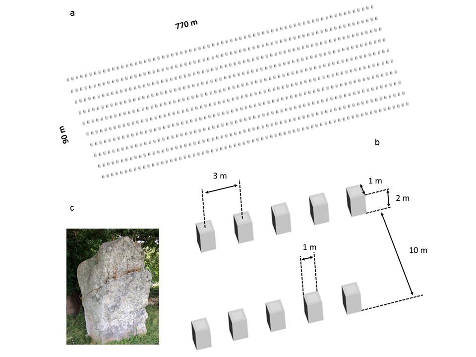
The Carnac stones are an exceptionally dense collection of megalithic sites in Brittany in northwestern France, consisting of stone alignments (rows), dolmens (stone tombs), tumuli (burial mounds) and single menhirs (standing alone stones). More than prehistoric standing stones were hewn from local granite and erected by the pre-Celtic people of Brittany. Most of the stones can be found within the Breton village of Carnac. The stones were erected at some stage during the Neolithic period, probably around BCE, but some may date to as early as BCE. The overall model is described on the basis of the two famous alignments of Ménec and Kermario. For instance, the Kermario alignment is made up of approximately menhirs distributed in 10 rows, over a distance of approximately m over approximately m wide. This set is generally oriented along a southwest-northeast
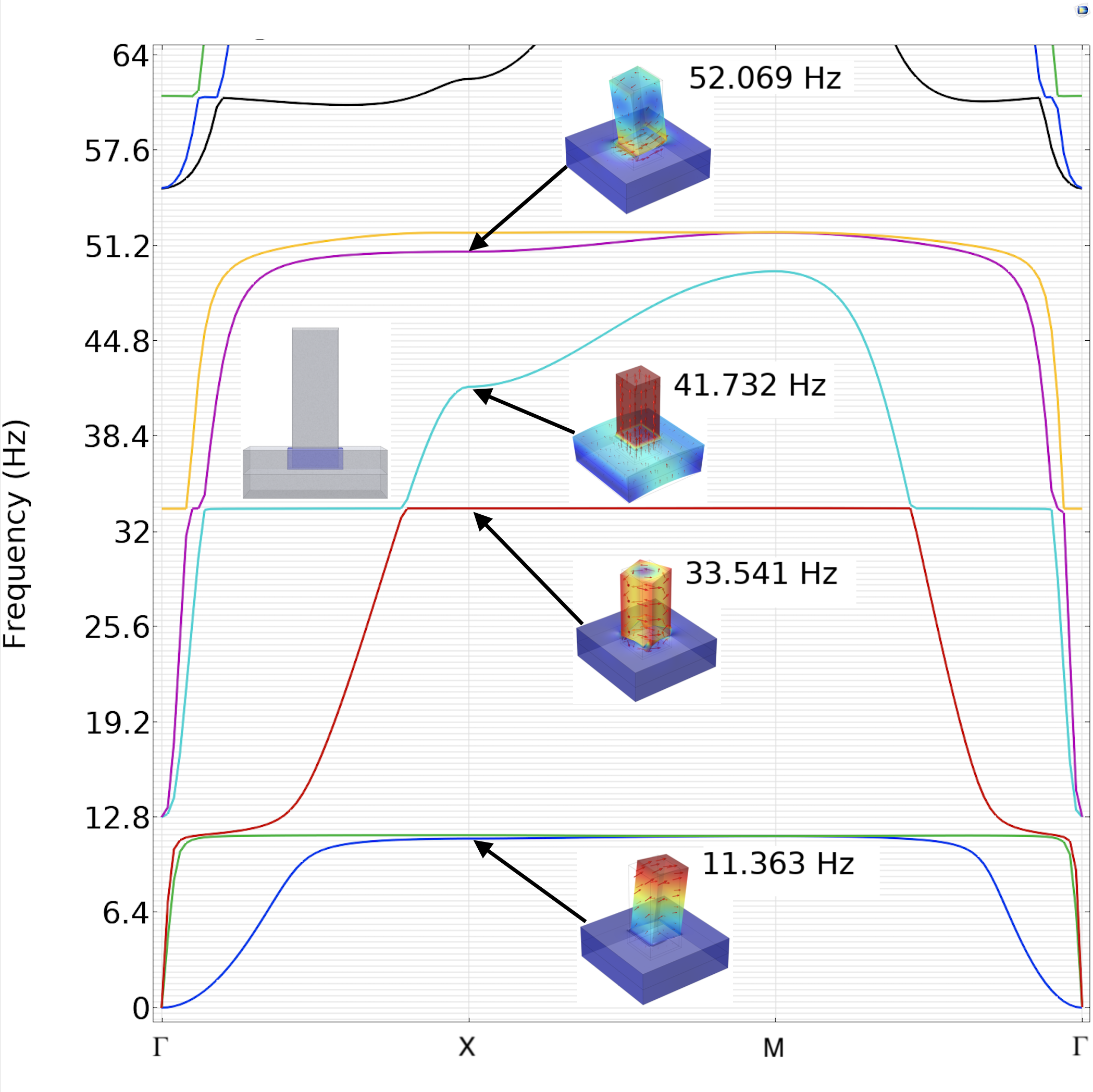
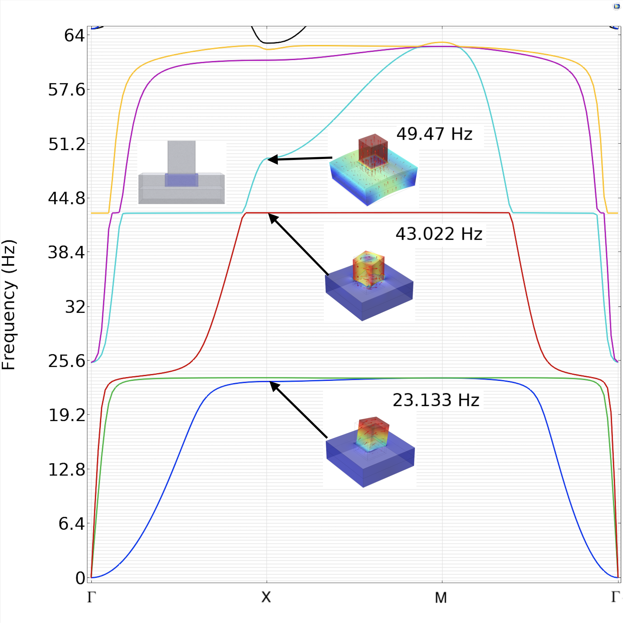
To set-up the model, we arbitrarily selected rows with a spacing of m between each stone. The height of the stones is m and their composition is local granite (density = kg.m-3) as well for the plate-model. The basic model is made of a set of stress-free cylindrical elements with a square-section ( m), which are clamped at one end (see Fig. 1).
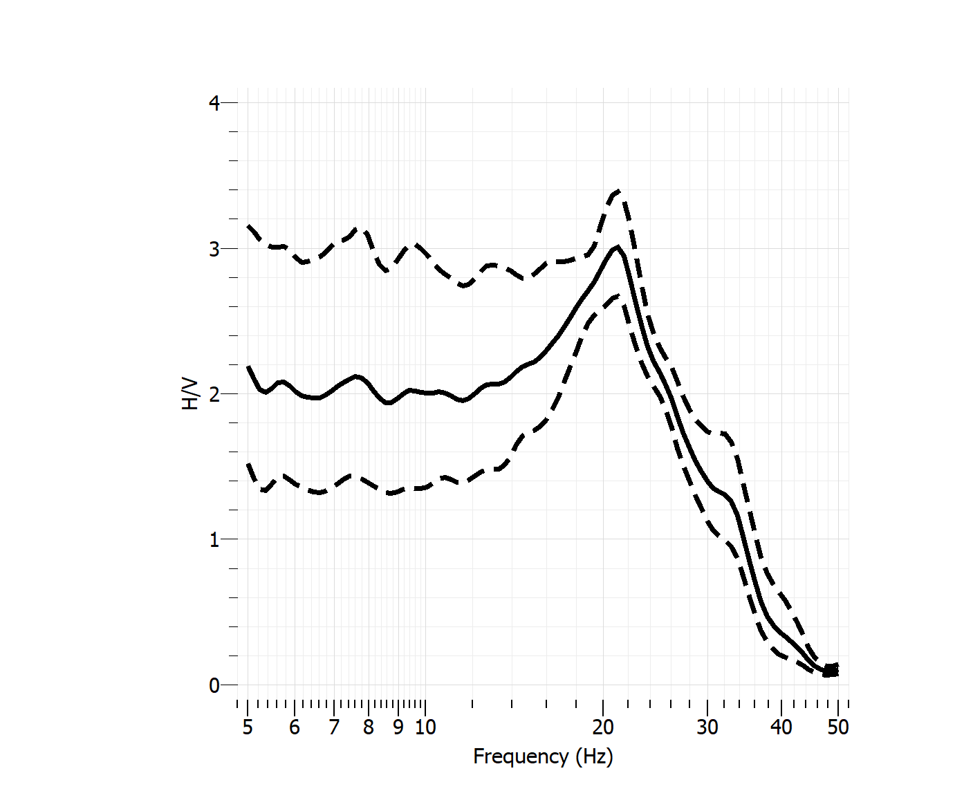
The local site conditions lead us to detail the initial clamped-free model. Indeed, standing stones are mainly placed on a granite base with a few tens of centimeters of topsoil (Figure 3). We define a topsoil thickness of m, at least, for parameter D in Figure 3. This depth is confirmed by archaeological studies Hinguant and Boujot (2017) but also by the HVSR measurements carried out on site. In fact, the peak frequency for the soil is identified around 20.6 Hz (Fig. 2) between two rows of stones. Assuming a shear wave velocity of m/s for the topsoil, we obtain m. D is assimilated to . The formula for the fundamental frequency of a 1D soil model laying on a seismic substratum is:
| (1) |
1D ground response analysis is based on the assumption that all boundaries are horizontal and that the response of a soil deposit is predominantly caused by SH-waves propagating vertically Brûlé et al. (2014).
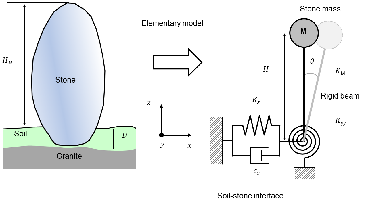
First, let consider a single degree-of-freedom elastic structure resting on a fixed base Clough and Penzien (1975) with the bending stiffness for a clamped-free beam, and mass (figure 3). From structural dynamics, the undamped natural vibration frequency, (rad/s), and period, (s), of the structure are given by:
| (2) |
and
| (3) |
Considering [6], i.e. m, MPa, m4, we find s or Hz. The clamping condition for this menhir induces a non realistic high frequency for the fundamental bending mode. Let us compare this analytical result with field measures by means of HVSR (figure 4).
Initiated by Nakamura in 1989 Nakamura (1989) and widely studied to explain its strengths and limitations Brûlé and Javelaud (2013); Bard et al. (2008); Bonnefoy-Claudet et al. (2006); Pilz et al. (2009) the seismological microtremor horizontal-to-vertical spectral ratio (HVSR) method offers a reliable estimation of the soil resonant frequencies from the spectral ratio between horizontal and vertical motions of microtremors (figure 2). This technique usually reveals the site dominant frequency but the interpretation of the amplitude of the HVSR is still an open question. The HVSR method was tested in geotechnical engineering too by virtue of its ease of use Brûlé and Javelaud (2013). In restrictive conditions, as for homogeneous soil layer model with a sharp acoustic impedance contrast with the seismic substratum, this technique could be employed to estimate the ground fundamental frequency . Ambient vibration techniques are also used for the determination of dynamic parameters of buildings Chatelain and Guillier (2013). Here, the method is employed to estimate both of the tested site, the dominant frequency of the bending mode of the menhir and the frequencies associated to the global dynamic response of the set of stones. Seismic noise was recorded with a sampling rate of Hz for 10 min at each site, this is to ensure that there is adequate statistical sampling in the range (0.1–50 Hz), the frequency range of engineering interest (TAB. 1 in Supplemental Material). HVSR curves are obtained with the open source Geopsy Software. Low-noise 20-s signal windows are selected through a short-term average (STA)/long-term average (LTA) antitrigger with 2-s STA, 30-s LTA, and low- and high-threshold of 0.2 and 3. A 5 percent cosine taper is applied to both ends of each time window on each component. The spectrum of each component of each individual window is smoothed according to the Konno and Ohmachi smoothing method Konno and Ohmachi (1998), using a constant of 40. Then, HVSR in each window is computed by merging the horizontal (north– south and east–west) components with a quadratic mean. Finally, HVSR is averaged over all selected windows.
Basically, the ratio of the H/V Fourier amplitude spectra is expressed with
| (4) |
where and denote the vertical and horizontal Fourier amplitude spectra respectively.
Different types of measures have been carried out on field. The sensors were placed on two stones to measure their local resonance (figure 4), at the foot of these to capture the signal emitted by themselves and at ground level, far from other stones to identify the specific geological site response (figure 1).
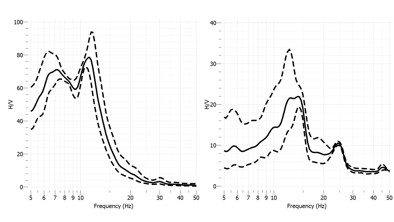
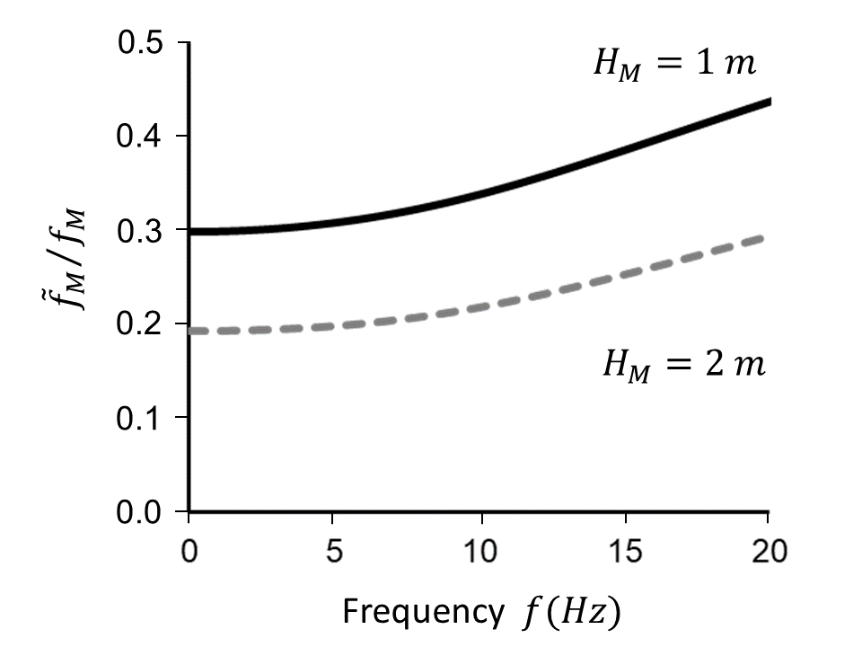
The measured frequency Hz for the 2 meter high stone and Hz for the 1 meter high one. These values are much lower than the theoretical ones for a perfectly clamped elastic model beam (equations 2 and 3). This difference can be explained by flexibility at the soil-structure interface, i.e. horizontal relative displacement and rigid body rotation (figure 3). Thus, we propose to introduce soil-structure interaction (SSI) to specify the parameters of the elementary model. This model is derived in Supplemental Material.
We had previously obtained Hz. According to figure 5, the SSI effect gives Hz. Thus the effect of the SSI is the lengthening of the period of the system. The equivalent height of the model is given by
| (5) |
We find m (to be compared with m) and m (to be compared with m).
Regarding the numerical simulations, performed with the commercial finite element software Comsol Multiphysics, we note the presence of low-frequency resonances of a rotational nature in-between the fundamental bending mode and longitudinal mode resonances in Fig. 6 and 7. The latter two are predicted by effective models such as in Marigo et al. (2021). However, the former has not been studied in great details yet, and seems to play a prominent role in the third resonance observed in Fig. 4, as suggested by the band diagram in Fig. 6.
In conclusion, the last decade is marked by the emergence of metamaterials including seismic metamaterials. Well beyond the important scientific and technological advances in the field of structured soils, the concepts of superstructures dynamically active under seismic stress and interacting with the supporting soils (soil kinematic effect) and its neighbors is clearly highlighted.
References
- Lalanne et al. (1999) P. Lalanne, S. Astilean, P. Chavel, E. Cambril, and H. Launois, JOSA A 16, 1143 (1999).
- Maier and Atwater (2005) S. A. Maier and H. A. Atwater, Journal of applied physics 98, 10 (2005).
- Zhu et al. (2017) A. Y. Zhu, A. I. Kuznetsov, B. Luk’yanchuk, N. Engheta, and P. Genevet, Nanophotonics 6, 452 (2017).
- Achaoui et al. (2011) Y. Achaoui, A. Khelif, S. Benchabane, L. Robert, and V. Laude, Physical Review B 83, 104201 (2011).
- Liu and Hussein (2012) L. Liu and M. I. Hussein, Journal of Applied Mechanics 79 (2012).
- Pourabolghasem et al. (2014) R. Pourabolghasem, A. Khelif, S. Mohammadi, A. A. Eftekhar, and A. Adibi, Journal of Applied Physics 116, 013514 (2014).
- Colombi et al. (2016a) A. Colombi, P. Roux, S. Guenneau, P. Gueguen, and R. V. Craster, Scientific reports 6, 19238 (2016a).
- Palermo et al. (2018) A. Palermo, S. Krödel, K. H. Matlack, R. Zaccherini, V. K. Dertimanis, E. N. Chatzi, A. Marzani, and C. Daraio, Physical Review Applied 9, 054026 (2018).
- Brûlé et al. (2019a) S. Brûlé, S. Enoch, and S. Guenneau, Nanophotonics 8, 1591 (2019a).
- Ungureanu et al. (2019) B. Ungureanu, S. Guenneau, Y. Achaoui, A. Diatta, M. Farhat, H. Hutridurga, R. V. Craster, S. Enoch, and S. Brûlé, EPJ Appl. Metamat. 6 (2019).
- Hajjaj and Tu (2022) M. M. Hajjaj and J. Tu, Comptes Rendus. Mécanique 350, 237 (2022).
- SESAME (2005) SESAME, Guidelines for the implementation of the H/V spectral ratio technique on ambient vibrations – measurements, processing and interpretations, European research project. deliverable D23.12 (2005).
- Merritt and Housner (1954) R. G. Merritt and G. W. Housner, Bulletin of the Seismological Society of America 44, 551 (1954).
- Housner (1957) G. W. Housner, Bulletin of the Seismological Society of America 47, 179 (1957).
- Brûlé et al. (2019b) S. Brûlé, S. Enoch, and S. Guenneau, Physics Letters A p. 126034 (2019b).
- Achaoui et al. (2017) Y. Achaoui, T. Antonakakis, S. Brule, R. Craster, S. Enoch, and S. Guenneau, New Journal of Physics 19, 063022 (2017).
- Colombi et al. (2016b) A. Colombi, D. Colquitt, P. Roux, S. Guenneau, and R. V. Craster, Scientific reports 6, 27717 (2016b).
- Colombi et al. (2017) A. Colombi, R. V. Craster, D. Colquitt, Y. Achaoui, S. Guenneau, P. Roux, and M. Rupin, Frontiers in Mechanical Engineering 3, 10 (2017).
- Achaoui et al. (2016) Y. Achaoui, B. Ungureanu, S. Enoch, S. Brûlé, and S. Guenneau, Extreme Mechanics Letters 8, 30 (2016).
- Krödel et al. (2015) S. Krödel, N. Thomé, and C. Daraio, Extreme Mechanics Letters 4, 111 (2015).
- Miniaci et al. (2016) M. Miniaci, A. Krushynska, F. Bosia, and N. M. Pugno, New Journal of Physics 18, 083041 (2016).
- Zeng et al. (2020) Y. Zeng, P. Peng, Q.-J. Du, Y.-S. Wang, and B. Assouar, Journal of Applied Physics 128, 014901 (2020).
-
Diosono et al. (2022)
F. Diosono,
A. Fraddosio,
A. La Notte,
N. Pecere, and
M. D. Piccioni, in
Living with Seismic Phenomena in the Mediterranean
and Beyond between Antiquity and the Middle Ages:
Proceedings of Cascia (25-26 October, 2019) and
Le Mans (2-3 June, 2021) Conferences (Archaeopress Publishing Ltd, 2022), p. 379. - Hinguant and Boujot (2017) P. S. Hinguant and C. Boujot, Dossiers d’Archéologie. Hors-Série pp. 52–53 (2017).
- Brûlé et al. (2014) S. Brûlé, E. Javelaud, S. Enoch, and S. Guenneau, Physical review letters 112, 133901 (2014).
- Clough and Penzien (1975) R. Clough and J. Penzien, Dynamics of Structures (McGraw Hill, 1975).
- Nakamura (1989) Y. Nakamura, Q. Rep. Railw. Tech. Res. Inst. 30, 25 (1989).
- Brûlé and Javelaud (2013) S. Brûlé and E. Javelaud, Revue française de Géotechnique pp. 3–15 (2013).
- Bard et al. (2008) P.-Y. Bard, J. L. Chazelas, P. Guéguen, M. Kham, and J. F. Semblat, in Assessing and managing earthquake risk (Springer, 2008), pp. 91–114.
- Bonnefoy-Claudet et al. (2006) S. Bonnefoy-Claudet, C. Cornou, P.-Y. Bard, F. Cotton, P. Moczo, J. Kristek, and D. Fäh, Geophysical Journal International 167, 827 (2006).
- Pilz et al. (2009) M. Pilz, S. Parolai, F. Leyton, J. Campos, and J. Zschau, Geophys. J. Int. 178(2), 713 (2009).
- Chatelain and Guillier (2013) J.-L. Chatelain and B. Guillier, Seismological Research Letters 84(2), 199 (2013).
- Konno and Ohmachi (1998) K. Konno and T. Ohmachi, Bulletin of the Seismological Society of America 88(1), 228 (1998).
- Marigo et al. (2021) J.-J. Marigo, K. Pham, A. Maurel, and S. Guenneau, Journal of Elasticity 146, 143 (2021).