Nearly Dimension-Independent Sparse Linear Bandit over Small Action Spaces via Best Subset Selection
Abstract
We consider the stochastic contextual bandit problem under the high dimensional linear model. We focus on the case where the action space is finite and random, with each action associated with a randomly generated contextual covariate. This setting finds essential applications such as personalized recommendation, online advertisement, and personalized medicine. However, it is very challenging as we need to balance exploration and exploitation. We propose doubly growing epochs and estimating the parameter using the best subset selection method, which is easy to implement in practice. This approach achieves regret with high probability, which is nearly independent in the “ambient” regression model dimension . We further attain a sharper regret by using the SupLinUCB framework and match the minimax lower bound of low-dimensional linear stochastic bandit problems. Finally, we conduct extensive numerical experiments to demonstrate the applicability and robustness of our algorithms empirically.
Keyword: Best subset selection, high-dimensional models, regret analysis, stochastic bandit.
1 Introduction
Contextual bandit problems receive significant attention over the past years in different communities, such as statistics, operations research, and computer science. This class of problems studies how to make optimal sequential decisions with new information in different settings, where we aim to maximize our accumulative reward, and we iteratively improve our policy given newly observed results. It finds many important modern applications such as personalized recommendation (Li et al., 2010, 2011), online advertising (Krause and Ong, 2011), cost-sensitive classification (Agarwal et al., 2014), and personalized medicine (Goldenshluger and Zeevi, 2013; Bastani and Bayati, 2015; Keyvanshokooh et al., 2019). In most contextual bandit problems, at each iteration, we first obtain some new information. Then, we take action based on a certain policy and observe a new reward. Our goal is to maximize the total reward, where we iteratively improve our policy. This paper is concerned with the linear stochastic bandit model, one of the most fundamental models in contextual bandit problems. We model the expected reward at each time period as a linear function of some random information depending on our action. This model receives considerable attention (Auer, 2002; Abe et al., 2003; Dani et al., 2008; Rusmevichientong and Tsitsiklis, 2010; Chu et al., 2011), and as we will discuss in more detail, it naturally finds applications in optimal sequential treatment regimes.
In a linear stochastic bandit model, at each time period , we are given some action space . Here each feasible action is associated with a -dimensional context covariate that is known before any action is taken. Next, we take an action and then observe a reward . Assume that the reward follows a linear model
| (1) |
where is an unknown -dimensional parameter, and are noises. Without loss of generality, we assume that we aim to maximize the total reward. We measure the performance of the selected sequence of actions by the accumulated regret
| (2) |
Essentially, the regret measures the difference between the “best” we can achieve if we know the true parameter and the “noiseless” reward we get. It is clear that regret is always nonnegative, and our goal is to minimize the regret.
Meanwhile, due to the advance of technology, there are many modern applications where we encounter the high-dimensionality issue, i.e., the dimension of the covariate is large. Note that here the total number of iterations is somewhat equivalent to the sample size, which is the number of pieces of information we are able to “learn” the true parameter . Such a high-dimensionality issue presents in practice. For example, given the genomic information of some patients, we aim to find a policy that assigns each patient to the best treatment for him/her. It is usually the case that the number of patients is much smaller than the dimension of the covariate. In this paper, we consider the linear stochastic contextual bandit problem under such a high-dimensional setting, where the parameter is of high dimension that . We assume that is sparse that only at most components of are non-zero. This assumption is commonly imposed in high-dimensional statistics and signal processing literature (Donoho, 2006; Bühlmann and Van De Geer, 2011).
In addition, for the action spaces , it is known in literature (Dani et al., 2008; Shamir, 2015; Szepesvari, 2016) that if there are infinitely many feasible actions at each iteration, the minimax lower bound is of order , which does not solve the curse of dimensionality. We assume that the action spaces are finite, small, and random. In particular, we assume that for all , , and each action in is associated with independently randomly generated contextual covariates. In most practical applications, this finite action space setting is naturally satisfied. For example, in the treatment example, there are usually only a small number of feasible treatments available. We refer the readers to Section 3.1 for a complete description and discussion of the assumptions.
1.1 Literature Review
We briefly review existing works on linear stochastic bandit problems under both low-dimensional and high-dimensional settings. Under the classical low-dimensional setting, Auer (2002) pioneers the use of upper-confidence-bound (UCB) type algorithms for the linear stochastic bandit, which is one of the most powerful and fundamental algorithms for this class of problems, and is also considered in Chu et al. (2011). Dani et al. (2008); Rusmevichientong and Tsitsiklis (2010) study linear stochastic bandit problems with large or infinite action spaces, and derive corresponding lower bounds. Under the high-dimensional setting, where we assume that is sparse, when the action spaces ’s are hyper-cube spaces , Lattimore et al. (2015) develop the SETC algorithm that attains nearly dimension-independent regret bounds. We point out that this algorithm exploits the unique structure of hyper-cubes and is unlikely to be applicable for general action spaces including the ones of our interest where the action spaces are finite. Abbasi-Yadkori et al. (2012) consider a UCB-type algorithm for general action sets and obtain a regret upper bound of , which depends polynomially on the ambient dimension . Note that here the notation is the big-O notation that ignores all logarithmic factors. Carpentier and Munos (2012) consider a different reward model and obtain an regret upper bound. Goldenshluger and Zeevi (2013); Bastani and Bayati (2015) study a variant of the linear stochastic bandit problem in which only one contextual covariate is observed at each time period , while each action corresponds to a different unknown model . We point out that this model is a special case of our model (1), as discussed in Foster et al. (2018).
Another closely related problem is the online sparse prediction problem (Gerchinovitz, 2013; Foster et al., 2016), in which sequential predictions ’s of are of the interest, and the regret is measured in mean-square error . It can be further generalized to online empirical-risk minimization (Langford et al., 2009) or even the more general derivative-free/bandit convex optimization (Nemirovsky and Yudin, 1983; Flaxman et al., 2005; Agarwal et al., 2010; Shamir, 2013; Besbes et al., 2015; Bubeck et al., 2017; Wang et al., 2017). Most existing works along this direction have continuous (infinite) action spaces . They allow small-perturbation type methods like estimating gradient descent. We summarize the existing theoretical results on stochastic linear bandit problems in Table 1.
From the application perspective of finding the optimal treatment regime, existing literatures focus on achieving the optimality through batch settings. General approaches include model-based methods such as Q-learning (Watkins and Dayan, 1992; Murphy, 2003; Moodie et al., 2007; Chakraborty et al., 2010; Goldberg and Kosorok, 2012; Song et al., 2015) and A-learning (Robins et al., 2000; Murphy, 2005) and model-free policy search methods (Robins et al., 2008; Orellana et al., 2010a, b; Zhang et al., 2012b; Zhao et al., 2012, 2014). These methods are all developed based on batch settings where we use the whole dataset to estimate the optimal treatment regime. This approach is applicable after the clinical trial is completed, or when the observational dataset is fully available. However, the batch setting approach is not applicable when it is emerging to identify the optimal treatment regime. For a contemporary example, during the recent outbreak of coronavirus disease (COVID-19), it is extremely important to quickly identify the optimal or nearly optimal treatment regime to assign each patient to the best treatment among a few choices. However, since the disease is novel, there is no or very little historical data. Thus, the batch setting approaches mentioned above are not applicable. On the other hand, our model naturally provides a “learn while optimizing” alternative approach to sequentially improve the policy/treatment regime. This provides an important motivating application of the proposed method.
1.2 Major Contributions
In this paper, we propose new algorithms, which iteratively learn the parameter while optimizing the regret. Our algorithms use the “doubling trick” and modern optimization techniques, which carefully balance the randomization for exploration to fully learn the parameter and maximizing the reward to achieve the near-optimal regret. In particular, our algorithms fall under the general UCB-type algorithms (Lai and Robbins, 1985; Auer et al., 2002). Briefly speaking, we start with some pure exploration periods that we take random actions uniformly, and we estimate the parameter. Then, for the next certain periods, which we call an epoch, we take the action at each time period by optimizing some upper confidence bands using the previous estimator. At the end of each epoch, we renew the estimator using new information. We then enter the next epoch using the new estimator and renew the estimator at the end of the next epoch. We repeat this until the -th time period.
The high-dimensional regime (i.e., ) poses significant challenges in our setting, which cannot be solved by exiting works. First, unlike in the low-dimensional regime where ordinary least squares (OLS) always admits closed-form solutions and error bounds, in the high-dimensional regime, most existing methods like the Lasso (Tibshirani, 1996) or the Dantzig selector (Candes and Tao, 2007) require the sample covariance matrix to satisfy certain restricted eigenvalue”conditions (Bickel et al., 2009), which do not hold under our setting for sequentially selected covariates. Additionally, our action spaces are finite. This rules out several existing algorithms, including the SETC method (Lattimore et al., 2015) that exploits the specific structure of hyper-cube actions sets and finite-difference type algorithms in stochastic sparse convex optimization (Wang et al., 2017; Balasubramanian and Ghadimi, 2018). We adopt the best subset selector estimator (Miller, 2002) to derive valid confidence bands only using ill-conditioned sample covariance matrices. Note that while the optimization for best subset selection is NP-hard in theory (Natarajan, 1995), by the tremendous progress of modern optimization, solving such problems is practically efficient as discussed in Pilanci et al. (2015); Bertsimas et al. (2016). In addition, the renewed estimator may correlate with the previous one. This decreases the efficiency. We let the epoch sizes grow exponentially, which is known as the “doubling trick” (Auer et al., 1995). This “removes” the correlation between recovered support sets by best subset regression. Our theoretical analysis is also motivated from some known analytical frameworks such as the elliptical potential lemma (Abbasi-Yadkori et al., 2011) and the SupLinUCB framework (Auer, 2002) in order to obtain sharp regret bounds.
We summarize our main theoretical contribution in the following corollary, which is essentially a simplified version of Theorem 2 in Section 3.3.
Corollary 1.
We assume that , , and , for each . Then there exists a policy such that with probability at least , for all and ,
where denotes a polynomial of logarithmic factors.
Note that this corollary holds even if . Theorem 2 provides more general results than this corollary, and can be applied for a broader family of distributions for contextual covariates . A simpler and more implementable algorithm, with a weaker regret guarantee of , is given in Algorithm 1 and Theorem 1, respectively. The form of regret guarantee in this Corollary 1 looks particularly similar to its low-dimensional counterparts in Table 1, with the ambient dimension replaced by the intrinsic dimension .
Notations. Throughout this paper, for an integer , we use to denote the set . We use to denote the and norms of vector, respectively. Given a matrix , we use to denote the norm weighted by . Specifically, we have . We also use to denote the inner product of two vectors. Given a set , is it complement and denotes the cardinality. Given a -dimensional vector , we use to denote its -th coordinate. We also use to represent the support of , which is the collection of indices corresponding to nonzero coordinates. Furthermore, we use to denote the restriction of on , which is a -dimensional vector. Similarly, for a matrix , we denote by the restriction of on , which is a matrix. When , we further abbreviate . In addition, given two sequences of nonnegative real numbers and , and mean that there exists an absolute constant such that and for all , respectively. We also abbreviate , if and hold simultaneously. We say that a random event holds with probability at least , if there exists some absolute constant such that the probability of is larger than . Finally, we remark that arm, action, and treatment all refer to actions in different applications. We also denote by the action taken in period and the associated covariate.
Paper Organization. The rest of this paper is organized as follows. We present our algorithms in Section 2. Then we establish our theoretical results in Section 3, under certain technical conditions. We conduct extensive numerical experiments using both synthetic and real datasets to investigate the performance of our methods in Section 4. We conclude the paper in Section 5.
2 Methodologies
In this section, we present the proposed methods to solve the linear stochastic bandit problem where we aim to minimize the regret defined in (2). In Section 2.1, we first introduce an algorithm called “Sparse-LinUCB” (SLUCB) as summarized in Alg. 1, which can be efficiently implemented, and demonstrate the core idea of our algorithmic design. The SLUCB algorithm is a variant of the celebrated LinUCB algorithm (Chu et al., 2011) for classical linear contextual bandit problems. The SLUCB algorithm is intuitive and easy to implement. However, we cannot derive the optimal upper bound for the regret. To close this gap, we further propose a more sophisticated algorithm called “Sparse-SupLinUCB” (SSUCB) (Alg. 2) in Section 3.2. In comparison with the SLUCB algorithm, the SSUCB algorithm constructs the upper confidence bands through sequentially selecting historical data and achieves the optimal rate (up to logarithmic factors).
2.1 Sparse-LinUCB Algorithm
As we mentioned above, our algorithm is inspired by the standard LinUCB algorithm, which balances the tradeoff between exploration and exploitation following the principle of “optimism in the face of uncertainty”. In particular, the LinUCB algorithm repeatedly constructs upper confidence bands for the potential rewards of the actions. The upper confidence bands are optimistic estimators. We then pick the action associated with the largest upper confidence band. This leads to the optimal regret under the low-dimensional setting. However, under the high-dimensional setting, directly applying the LinUCB algorithm incurs some suboptimal regret since we only get lose confidence bands under the high-dimensional regime. Thus, it is desirable to construct tight confidence bands under the high-dimensional and sparse setting to achieve the optimal regret.
Inspired by the remarkable success of the best subset selection (BSS) in high-dimensional regression problems, we propose to incorporate this powerful tool into the LinUCB algorithm. Meanwhile, since the BSS procedure is computationally expensive, it is impractical to execute the BSS method during every time period. In addition, as we will discuss later, it is not necessary.
Before we present our algorithms, we briefly discuss the support of parameters. Given a -dimensional vector , we denote by the support set of , which is the collection of dimensions of with nonzero coordinates that
This definition agrees with that of most literatures. However, for the BSS procedure, it is desirable to generalize this definition. We propose the concept of “generalized support” as follows.
Definition 1 (Generalized Support).
Given a -dimensional vector , we call a subset the generalized support of and denote it by , if
The generalized support is a relaxation of the normal support, since any support is a generalized support (but not vice versa). Moreover, the generalized support is not unique. Any subset including the support is a valid generalized support.
We distinguish the difference between support and generalized support in order to define the best subset selection without causing confusion. For example, we consider a linear model , and . Calculating the ordinary least square estimator restricted on the generalized support , which is denoted by
means that we consider a low-dimensional model only using the information in and set the coordinates of estimator except in as zeros. Formally, let be
Then we have
Since we do not guarantee , we call the generalized support instead of support.
We are ready to present the details of SLUCB algorithm now. Our algorithm works as follows. We first apply the “doubling trick”, which partitions the whole decision periods into several consecutive epochs such that the lengths of the epochs increase doubly. We only implement the BSS procedure at the end of each epoch to recover the support of the parameter . Within each epoch, we start with a minimal epoch length of for pure exploration, which is called the pure-exploration-stage. At each time period of this stage, we pick an action within uniformly at random. Intuitively speaking, in pure-exploration-stage, we explore the unknown parameters at all possible directions through uniform randomization. From a technical perspective, the pure-exploration-stage is desirable since it maintains the smallest sparse eigenvalue of the empirical design matrix lower bounded away from zero and hence, help us obtain an efficient estimator for . After the pure-exploration-stage, we keep the estimated support, say of nonzero components, from the previous epoch unchanged, and treat the problem as an -dimensional regression. Specifically, at each time period, we use the ridge estimator with penalty weight to estimate and construct corresponding confidence bands to help us make decisions in the next time period.
In summary, we partition the time horizon into consecutive epochs such that
The length of the last epoch may be less than or . By definition, the number of epochs . Hence, in the SLUCB algorithm, we run the BSS procedure times. In our later simulations studies, we find that this is practical for moderately large dimensions.
Next, we introduce the details of constructing upper confidence bands in the SLUCB algorithm. We assume that at period , we pick action and observe the associated covariate and reward . We also abbreviate as , if there is no confusion. We denote by the BSS estimator for the true parameter at the end of previous epoch , and let
be its generalized support, i.e., the generalized support recovered by epoch . For periods in the pure-exploration-stage of , we pick arms uniformly at random and do not update the estimator of . Beyond the pure-exploration-stage, we estimate by a ridge estimator. Let be the most updated ridge estimator of by , which is estimated by restricting its generalized support on using data . In particular, all components of outside are set as zeros and
Given , we calculate the upper confidence band of potential reward for each possible action . In particular, let the tuning parameters and be
which correspond to the confidence level and upper estimate of potential reward, respectively. Then we calculate the upper confidence band associated with action as
where
After that, we pick the arm corresponding to the largest upper confidence band to play and observe the corresponding reward . We repeat this process until the end of epoch .
Then we run the BSS procedure using all data collected in to recover the support of . We also enlarge the size of generalized support by . To be specific, let be the generalized support recovered in this step. We require that satisfies constraints
and obtain the BSS estimator as
| (3) |
where denotes the projection on a centered -ball with radius , the -norm of . Note that in comparison with the standard BSS estimator, we project the minimizer for regularization. The boundedness also simplifies our later theoretical analysis. We also add the inclusion restriction for some technical reasons, which does not lead to any fundamental difference. As a result, we need to consider the sparsity instead of . It boosts the probability of recovering the true support.
A pseudo-code description of the SLUCB algorithm is presented in Algorithm 1. We remark that although computing the BSS estimator is computationally expensive, many methods exist that can solve this problem very efficiently in practice. See, for example, (Pilanci et al., 2015; Bertsimas et al., 2016) for more details. We also conduct extensive numerical experiments to demonstrate that our proposed algorithm is practical in Section 4.
2.2 Sparse-SupLinUCB Algorithm
Although the SLUCB algorithm is intuitive and easy to implement, we are unable to prove the optimal upper bound for its regret due to some technical reasons. Specifically, as discussed in the next section, we can only establish an upper bound for the regret of the SLUCB algorithm, while the optimal regret should be . Here we omit all the constants and logarithmic factors and only consider the dependency on horizon length and dimension parameters. The obstacle leading to sub-optimality is the dependency of covariates on random noises. Recall that at each period , the SLUCB algorithm constructs the ridge estimator using all historical data, where designs are correlated with noises due to the UCB-type policy. Such a complicated correlation impedes us from establishing tight confidence bands for predicted rewards, which results in suboptimal regret.
To close the aforementioned gap and achieve the optimality, we modify the seminal SupLinUCB algorithm (Auer, 2002; Chu et al., 2011), which is originally proposed to attain the optimal regret for classic stochastic linear bandit problem, as a subroutine in our framework. Then we propose the Sparse-SupLinUCB (SSUCB) algorithm. Specifically, we replace the ridge estimator and UCB-type policy with a modified SupLinUCB algorithm. The basic idea of the SupLinUCB algorithm is to separate the dependent designs into several groups such that within each group, the designs and noises are independent of each other. Then the ridge estimators of the true parameters are calculated based on group individually. Thanks to the desired independency, now we can derive tighter confidence bands by applying sharper concentration inequality, which gives rise to the optimal regret in the final.
In the next, we present the details of SupLinUCB algorithm and show how to embed it in our framework. For each period that belongs to the UCB-stage, the SupLinUCB algorithm partitions the historical periods into disjoint groups
where . These groups are initialized by evenly partitioning periods from the pure-exploration-stage and are updated sequentially following the rule introduced as follows. For each period , we screen the groups one by one (in an ascending order of index ) to determine the action to take or eliminate some obvious sub-optimal actions.
Suppose that we are at the -th group now. Let be the set of candidate actions that are still kept by the -th step, which is initialized as the whole action space when . We first calculate the ridge estimator restricted on the generalized support , using data from group . Then for each action , we calculate , the width of confidence band of the potential reward. Specifically, we have
where the tuning parameter
corresponds to the confidence level. Our next step depends on the values of . If
which means that the widths of confidence bands are uniformly small, we pick the action associated with the largest upper confidence band
where is an upper estimate of potential rewards. In this case, we discard the data point and do not update any group, i.e., setting , for all
Otherwise, if there exists some such that which means that the width of confidence band is not sufficiently small, then we pick such an action to play for exploration. In this case, we add the period into the -th group while keeping all other groups unchanged, i.e.,
Finally, if neither one of the above scenarios happens, which implies that for all , then we do not take any action for now. Instead, we eliminate some obvious sub-optimal actions and move to the next group . Particularly, we update the set of candidate arms as
We repeat the above procedure until an arm is selected. Since the number of groups is and , the SupLinUCB algorithm stops eventually. Finally, by replacing the direct ridge regression and UCB-type policy with the SupLinUCB algorithm above, we obtain the SSUCB algorithm. The pseudo-code is presented in Algorithm 2.
3 Theoretical Results
In this section, we present the theoretical results of the SLUCB and SSUCB algorithms. We use the regret to evaluate the performance of our algorithms, which is a standard performance measure in literature. We denote by the actions sequence generated by an algorithm. Then given the true parameter and covariates , the regret of the sequence is defined as
| (4) |
where denotes the optimal action under the true parameter. The regret measures the discrepancy in accumulated reward between real actions and oracles where the true parameter is known to a decision-maker. In what follows, in Section 3.1, we first introduce some technical assumptions to facilitate our discussions. Then we study the regrets of the SLUCB and SSUCB algorithms in Section 3.2 and Section 3.3, respectively.
3.1 Assumptions
We present the assumptions in our theoretical analysis and discuss their relevance and implications. We consider finite action spaces and assume that there exists some constant such that
We also assume that for each period , the covariates are sampled independently from an unknown distribution . We further impose the following assumptions on distribution .
Assumption 1.
Let random vector follow the distribution . Then satisfies:
-
(A1)
(Sub-Gaussianity): Random vector is centered and sub-Gaussian with parameter , which means that and
-
(A2)
(Non-degeneracy): There exists a constant such that
-
(A3)
(Independent coordinates): The coordinates of are independent of each other.
We briefly discuss Assumption 1. First of all, (A1) is a standard assumption in literature, with sub-Gaussianity covering a broad family of distributions like Gaussian, Rademacher, and bounded distributions. Assumption (A2) is a non-degeneracy assumption which, together with (A3), implies that the smallest eigenvalue of the population covariance matrix is lower bounded by some constant . Similar assumptions are also adopted in high-dimensional statistics literature in order to prove the “restricted eigenvalue” conditions of sample covariance matrices (Raskutti et al., 2010), which are essential in the analysis of penalized least square methods (Wainwright, 2009; Bickel et al., 2009). However, we emphasize that in this paper the covariates indexed by the selected actions do not satisfy the restricted eigenvalue condition in general, and therefore, we need novel and non-standard analyses of high-dimensional M-estimators. For Assumption (A3), at a higher level, independence among coordinates enables relatively independent explorations in different dimensions, which is similar to the key idea of the SETC method (Lattimore et al., 2015). Technically, (A3) is used to establish the key independence of sample covariance matrices restricted within and outside the recovered support. Due to such an independence, the rewards in the unexplored directions at each period are independent as well, which can be estimated efficiently.
We also impose the following assumptions on the unknown -dimensional true parameter .
Assumption 2.
-
(B1)
(Sparsity): The true parameter is sparse. In other words, there exists an such that .
-
(B2)
(Boundedness): There exists a constant such that .
Note that in Assumption 2, (B1) is the key sparsity assumption, which assumes that only components of the true parameter are non-zero. Assumption (B2) is a boundedness condition on the -norm of . This assumption is often imposed, either explicitly or implicitly, in contextual bandit problems for deriving an upper bound for rewards (Dani et al., 2008; Chu et al., 2011).
Finally, we impose the sub-Gaussian assumption on noises sequence , which is a standard assumption adopted in most statistics and bandit literatures.
Assumption 3.
-
(C1)
(Sub-gaussian noise): The random noises are independent, centered, and sub-Gaussian with parameter .
3.2 Regret Analysis of Sparse-LinUCB
In this section, we analyze the performance of the SLUCB algorithm. As discussed earlier, we measure the performance via the regret defined in (4). We show that with a tailored choice of pure-exploration-stage length , tuning parameters , and , the accumulated regret of the SLUCB algorithm is upper bounded by (up to logarithmic factors) with high probability. Formally, we have the following theorem.
Theorem 1.
Note that in Theorem 1, if we omit all the constants and logarithmic factors, the dominating part in the accumulated regret is
Theorem 1 builds on a nontrivial combination of the UCB-type algorithm and the best subset selection method. To save space, we put the complete proof of Theorem 1 in Appendix A.
3.3 Regret Analysis of Sparse-SupLinUCB
In comparison with the SLUCB algorithm, the SSUCB algorithm splits the historical data into several groups dynamically. In each period, we sequentially update the ridge estimator and corresponding confidence bands using data from a single group instead of the whole data. The motivation of only using a single group of data is to achieve the independence between the design matrix and random noises within each group, which leads to tighter confidence bands by applying a sharper concentration inequality. The tighter upper bounds of the predicted rewards lead to an improved regret. In particular, we have the following theorem.
Theorem 2.
Note that in Theorem 2, if we omit all constants and logarithmic factors, the dominating part in the regret upper bound is of order . This improves the rate in Theorem 1 by an order of and achieves the optimal rate (up to logarithmic factors). Theorem 2 builds on a tailored analysis of the SupLinUCB algorithm. To save space, we also put the complete proof of Theorem 2 in Appendix B.
4 Numerical Experiments
In this section, we use extensive numerical experiments to demonstrate our proposed algorithm’s efficiency and validate our theoretical results. To simplify implementation, we only test the SLUCB algorithm in our experiments, which can be implemented efficiently. Theoretically, the SLUCB algorithm only achieves a sub-optimal regret guarantee due to technical reasons. However, extensive numerical experiments imply that it attains the near-optimality in practice. Specifically, we first empirically verify the regret guarantee established in Section 3 via simulation under various settings. Then we apply the proposed method to a sequential treatment assignment problem using a real medical dataset. In simulation studies, we sample the contextual covariates from -dimensional standard Gaussian distribution. For the real dataset test, we sample the covariates from the empirical distribution, which may not be Gaussian. Some assumptions in Section 3.1 are also violated. However, in all scenarios, our algorithm performs well and achieves regrets, which demonstrates the robustness and practicability.
4.1 Simulation Studies
In this section, we present the details of our simulation studies. We first show the growth rate of regret empirically. Then we fix time horizon length and dimension and study the dependency of accumulated regret on sparsity . To demonstrate the power of best subset selection, we also compare our algorithm’s performance with the oracle, where the decision-maker knows the true support of underlying parameters. Since the bottleneck of computing time in our algorithm is the best subset selection, which requires solving a mixed-integer programming problem, it is appealing to replace this step with other variable selection methods, such as Lasso and iterative hard thresholding (IHT) (Blumensath and Davies, 2009). So we test the performance of those variants. We fix the number of actions in all settings.
4.1.1 Experiment 1: Growth of regret
In this experiment, we study the growth rate of regret. We run two sets of experiments, where in the first case and in the second case, . For each setup, we replicate times and then calculate corresponding mean and -confidence interval. We present the results in Figure 1. As we see, for each fixed and , the growth rate of regret is about , which validates our theory.
 |
 |
4.1.2 Experiment 2: Dependency on sparsity
In this experiment, we fix the dimension and horizon length and let sparsity varies. We calculate the accumulated regret at the end of horizon. We also run two sets of experiments, where in the first case and in the second case . We present the results are presented in Figure 2. Although Theorem 1 only provides an regret guarantee for the SLUCB algorithm. The linear dependency of accumulated regret on suggests that it actually attains the optimal rate in practice.
 |
 |
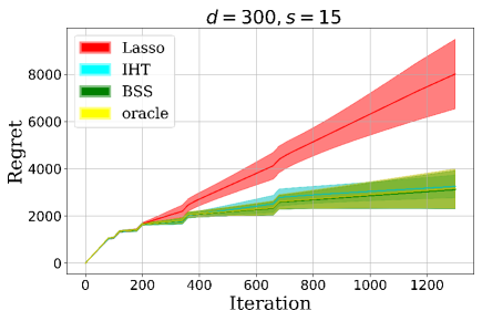
4.1.3 Experiment 3: Comparison with variants of main algorithm and oracle
In this experiment, we compare the performance and the computing time of our algorithm with several variants that substitute the best subset selection subroutine with Lasso and IHT. We also compare with the oracle regret where the decision-maker knows the true support of parameters. In more detail, for the first variant, we use Lasso to recover the support of the true parameter at the end of each epoch. We tune the -penalty such that the size of the support of the estimator is approximately equal to , and then use it in the next epoch. For the second variant, we apply IHT to estimate the parameter and set the hard threshold to be .
We run two settings of experiments, corresponding to , and . We also replicate times in each setting. For the first case, the averaged computing times are seconds for Lasso, seconds for IHT, and seconds for best subset selection. For the second case, the average computing times are seconds for Lasso, seconds for IHT, and seconds for best subset selection. We display the associated regret curves in Figure 3. As we see, although the computing time of Lasso is shorter than the other two methods, the performance of Lasso is significantly weaker. The computing time of IHT is slightly longer than Lasso, but it achieves the similar performance as best subset selection, which suggests that IHT might be a good alternative in practice when the computing resource is limited. Finally, although the computing time of the best subset selection is the longest, its performance is the best. The regret almost achieves the same performance as the oracle. Such a result demonstrates the power of best subsection selection in high-dimensional stochastic bandit problems.
 |
 |
4.2 Real Dataset Test
In this section, we apply our methods in a sequential treatment assignment problem based on the ACTG175 dataset from the R package “speff2trial”. The scenario is that patients arrive at a clinic sequentially. Several candidate treatments are available, and different treatments may have different treatment effects. Hence, for each patient, the doctor observes his/her health information and then chooses a treatment for the patient, to maximize the total treatment effect.
We first briefly introduce the ACTG175 dataset (Hammer et al., 1996). This dataset records the results of a randomized experiment on 2139 HIV-infected patients, and the background information of those patients. The patients are randomly assigned one of the four treatments: zidovudine (AZT) monotherapy, AZT+didanosine (ddI), AZT+zalcitabine (ddC), and ddI monotherapy. The treatment effect is measured via the number of CD8 T-cell after 20 weeks of therapy. Besides, for each patient, an -dimensional feature vector is provided as the background information, which includes age, weight, gender, drug history, etc.
Similar to the simulation studies, we validate our algorithms by regret. However, in practice, the potential outcomes of unassigned treatments on each patient are unavailable, which prevents us from calculating the regret. To overcome this difficulty, we assume a linear model for the treatment effect of each therapy. Particularly, we assume that the effect of treatment (number of CD8 T cell) is , where denotes the background information of each patient, is a standard Gaussian noise, and is estimated via linear regression. Similar assumptions are commonly adopted in statistics literatures to calculate the counterfactual, when real experiments are unavailable (Zhang et al., 2012a). Above sequential treatment assignment problem can be easily transformed to our formulation by considering the joint covariate and space. Given a patient with background , let , and . Since , assigning treatment to a patient is equivalent to pick an action from space . Note that with this formulation, Assumption 1 is violated. However, the numerical results introduced below still demonstrate the good performance of our algorithm.
 |
In this experiment, for simplicity, we pick coordinates (age, weight, drugs in history, Karnofsky score, number of days of previously received antiretroviral therapy, antiretroviral history stratification, gender, CD4 T cell number at baseline, and CD8 T cell number at baseline), from the whole dataset as the covariate. We denote by it . Then we use the real dataset to estimate the true parameters , i.e., the treatment effect of each therapy. To test our algorithm in the high dimensional setting, we further concatenate with a -dimensional random noise drawn from standard Gaussian distribution. The parameters corresponding to those injected noises are zeros. For each patient, we use the estimated parameters to calculate the potential treatment effect and regret. In addition, we choose the total number of patients . Like the simulation studies, we compare our algorithm’s performance with other variants (Lasso,IHT, and oracle). For each algorithm, we repeat times and calculate the mean regret curve. We present the result in Figure 4. Compared with the simulation studies, the performance of Lasso is still the worst. However, the discrepancy is much smaller. Although there is almost no difference in IHT and best subset selection, in real data tests, we may observe some instances where the IHT algorithm fails to converge, which means a lack of robustness. Again, for our proposed algorithm, we observe an growth rate of regret. It is pretty close to the oracle as well. So The BSS algorithm also achieves the optimality. Since in this experiment, technical assumptions in Section 3.1 are violated, the numerical results demonstrate the robustness of our method.
5 Conclusion
In this paper, we first propose a method for the high-dimensional stochastic linear bandit problem by combining the best subset selection method and the LinUCB algorithm. It achieves the regret upper bound and is nearly independent with the ambient dimension (up to logarithmic factors). In order to attain the optimal regret , we further improve our method by modifying the SupLinUCB algorithm. Extensive numerical experiments validate the performance and robustness of our algorithms. Moreover, although we cannot prove the regret upper bound for the SLUCB algorithm due to some technical reasons, simulation studies show that the regret of SLUCB algorithm is actually rather than our provable upper bound . A similar phenomenon is also observed in the seminal works (Auer, 2002; Chu et al., 2011), where low-dimensional stochastic linear bandit problems are investigated. It remains an open problem to prove the upper bound for the LinUCB-type algorithms. In addition, it is also interesting to study the high-dimensional stochastic linear bandit problem under weaker assumptions, especially when the independent coordinates assumption does not hold. We view all of those problems as potential future research directions.
References
- Abbasi-Yadkori et al. [2011] Y. Abbasi-Yadkori, D. Pál, and C. Szepesvári. Improved algorithms for linear stochastic bandits. In Advances in Neural Information Processing Systems, pages 2312–2320, 2011.
- Abbasi-Yadkori et al. [2012] Y. Abbasi-Yadkori, D. Pal, and C. Szepesvari. Online-to-confidence-set conversions and application to sparse stochastic bandits. In Proceedings of International Conference on Artificial Intelligence and Statistics (AISTATS), 2012.
- Abe et al. [2003] N. Abe, A. W. Biermann, and P. M. Long. Reinforcement learning with immediate rewards and linear hypotheses. Algorithmica, 37(4):263–293, 2003.
- Agarwal et al. [2010] A. Agarwal, O. Dekel, and L. Xiao. Optimal algorithms for online convex optimization with multi-point bandit feedback. In Proceedings of annual Conference on Learning Theory (COLT). Citeseer, 2010.
- Agarwal et al. [2014] A. Agarwal, D. Hsu, S. Kale, J. Langford, L. Li, and R. Schapire. Taming the monster: A fast and simple algorithm for contextual bandits. In Proceedings of International Conference on Machine Learning (ICML), 2014.
- Auer [2002] P. Auer. Using confidence bounds for exploitation-exploration trade-offs. Journal of Machine Learning Research, 3(Nov):397–422, 2002.
- Auer et al. [1995] P. Auer, N. Cesa-Bianchi, Y. Freund, and R. E. Schapire. Gambling in a rigged casino: The adversarial multi-armed bandit problem. In Proceedings of the IEEE Symposium on Foundations of Computer Science (FOCS), 1995.
- Auer et al. [2002] P. Auer, N. Cesa-Bianchi, and P. Fischer. Finite-time analysis of the multiarmed bandit problem. Machine Learning, 47(2-3):235–256, 2002.
- Balasubramanian and Ghadimi [2018] K. Balasubramanian and S. Ghadimi. Zeroth-order (non)-convex stochastic optimization via conditional gradient and gradient updates. In Proceedings of Advances in Neural Information Processing Systems (NIPS), 2018.
- Bastani and Bayati [2015] H. Bastani and M. Bayati. Online decision-making with high-dimensional covariates. 2015. Available at SSRN: https://ssrn.com/abstract=2661896.
- Bertsimas et al. [2016] D. Bertsimas, A. King, and R. Mazumder. Best subset selection via a modern optimization lens. The Annals of Statistics, 44(2):813–852, 2016.
- Besbes et al. [2015] O. Besbes, Y. Gur, and A. Zeevi. Non-stationary stochastic optimization. Operations Research, 63(5):1227–1244, 2015.
- Bickel et al. [2009] P. J. Bickel, Y. Ritov, and A. B. Tsybakov. Simultaneous analysis of lasso and dantzig selector. The Annals of Statistics, 37(4):1705–1732, 2009.
- Blumensath and Davies [2009] T. Blumensath and M. E. Davies. Iterative hard thresholding for compressed sensing. Applied and computational harmonic analysis, 27(3):265–274, 2009.
- Bubeck et al. [2017] S. Bubeck, Y. T. Lee, and R. Eldan. Kernel-based methods for bandit convex optimization. In Proceedings of the Annual ACM SIGACT Symposium on Theory of Computing (STOC), 2017.
- Bühlmann and Van De Geer [2011] P. Bühlmann and S. Van De Geer. Statistics for high-dimensional data: methods, theory and applications. Springer Science & Business Media, 2011.
- Candes and Tao [2007] E. Candes and T. Tao. The dantzig selector: Statistical estimation when p is much larger than n. The Annals of Statistics, 35(6):2313–2351, 2007.
- Carpentier and Munos [2012] A. Carpentier and R. Munos. Bandit theory meets compressed sensing for high dimensional stochastic linear bandit. In Proceedings of International Conference on Artificial Intelligence and Statistics (AISTATS), 2012.
- Chakraborty et al. [2010] B. Chakraborty, S. Murphy, and V. Strecher. Inference for non-regular parameters in optimal dynamic treatment regimes. Statistical Methods in Medical Research, 19(3):317–343, 2010.
- Chu et al. [2011] W. Chu, L. Li, L. Reyzin, and R. Schapire. Contextual bandits with linear payoff functions. In Proceedings of the International Conference on Artificial Intelligence and Statistics (AISTATS), 2011.
- Dani et al. [2008] V. Dani, T. P. Hayes, and S. M. Kakade. Stochastic linear optimization under bandit feedback. In Proceedings of annual Conference on Learning Theory (COLT), 2008.
- Donoho [2006] D. L. Donoho. Compressed sensing. IEEE Transactions on Information Theory, 52(4):1289–1306, 2006.
- Filippi et al. [2010] S. Filippi, O. Cappe, A. Garivier, and C. Szepesvári. Parametric bandits: The generalized linear case. In Proceedings of Advances in Neural Information Processing Systems (NIPS), 2010.
- Flaxman et al. [2005] A. D. Flaxman, A. T. Kalai, and H. B. McMahan. Online convex optimization in the bandit setting: gradient descent without a gradient. In Proceedings of the annual ACM-SIAM symposium on Discrete algorithms (SODA), 2005.
- Foster et al. [2016] D. Foster, S. Kale, and H. Karloff. Online sparse linear regression. In Proceedings of annual Conference on Learning Theory (COLT), 2016.
- Foster et al. [2018] D. J. Foster, A. Agarwal, M. Dudík, H. Luo, and R. E. Schapire. Practical contextual bandits with regression oracles. In Proceedings of the International Conference on Machine Learning (ICML), 2018.
- Gerchinovitz [2013] S. Gerchinovitz. Sparsity regret bounds for individual sequences in online linear regression. Journal of Machine Learning Research, 14(Mar):729–769, 2013.
- Goldberg and Kosorok [2012] Y. Goldberg and M. R. Kosorok. Q-learning with censored data. Annals of Statistics, 40(1):529, 2012.
- Goldenshluger and Zeevi [2013] A. Goldenshluger and A. Zeevi. A linear response bandit problem. Stochastic Systems, 3(1):230–261, 2013.
- Hammer et al. [1996] S. M. Hammer, D. A. Katzenstein, M. D. Hughes, H. Gundacker, R. T. Schooley, R. H. Haubrich, W. K. Henry, M. M. Lederman, J. P. Phair, M. Niu, et al. A trial comparing nucleoside monotherapy with combination therapy in hiv-infected adults with cd4 cell counts from 200 to 500 per cubic millimeter. New England Journal of Medicine, 335(15):1081–1090, 1996.
- Keyvanshokooh et al. [2019] E. Keyvanshokooh, M. Zhalechian, C. Shi, M. P. Van Oyen, and P. Kazemian. Contextual learning with online convex optimization: Theory and application to chronic diseases. Available at SSRN, 2019.
- Krause and Ong [2011] A. Krause and C. S. Ong. Contextual gaussian process bandit optimization. In Proceedings of Advances in Neural Information Processing Systems (NIPS), 2011.
- Lai and Robbins [1985] T. L. Lai and H. Robbins. Asymptotically efficient adaptive allocation rules. Advances in Applied Mathematics, 6(1):4–22, 1985.
- Langford et al. [2009] J. Langford, L. Li, and T. Zhang. Sparse online learning via truncated gradient. Journal of Machine Learning Research, 10(Mar):777–801, 2009.
- Lattimore et al. [2015] T. Lattimore, K. Crammer, and C. Szepesvári. Linear multi-resource allocation with semi-bandit feedback. In Proceedings of Advances in Neural Information Processing Systems (NIPS), 2015.
- Li et al. [2010] L. Li, W. Chu, J. Langford, and R. E. Schapire. A contextual-bandit approach to personalized news article recommendation. In Proceedings of the International Conference on World Wide Web (WWW). ACM, 2010.
- Li et al. [2011] L. Li, W. Chu, J. Langford, and X. Wang. Unbiased offline evaluation of contextual-bandit-based news article recommendation algorithms. In Proceedings of the ACM International Conference on Web Search and Data Mining (WSDM). ACM, 2011.
- Li et al. [2017] L. Li, Y. Lu, and D. Zhou. Provably optimal algorithms for generalized linear contextual bandits. In Proceedings of International Conference on Machine Learning (ICML), 2017.
- Miller [2002] A. Miller. Subset selection in regression. Chapman and Hall/CRC, 2002.
- Moodie et al. [2007] E. E. Moodie, T. S. Richardson, and D. A. Stephens. Demystifying optimal dynamic treatment regimes. Biometrics, 63(2):447–455, 2007.
- Murphy [2003] S. A. Murphy. Optimal dynamic treatment regimes. Journal of the Royal Statistical Society: Series B (Statistical Methodology), 65(2):331–355, 2003.
- Murphy [2005] S. A. Murphy. An experimental design for the development of adaptive treatment strategies. Statistics in medicine, 24(10):1455–1481, 2005.
- Natarajan [1995] B. K. Natarajan. Sparse approximate solutions to linear systems. SIAM Journal on Computing, 24(2):227–234, 1995.
- Nemirovsky and Yudin [1983] A. S. Nemirovsky and D. B. Yudin. Problem complexity and method efficiency in optimization. SIAM, 1983.
- Orellana et al. [2010a] L. Orellana, A. Rotnitzky, and J. M. Robins. Dynamic regime marginal structural mean models for estimation of optimal dynamic treatment regimes, part I: main content. The International Journal of Biostatistics, 6(2), 2010a.
- Orellana et al. [2010b] L. Orellana, A. Rotnitzky, and J. M. Robins. Dynamic regime marginal structural mean models for estimation of optimal dynamic treatment regimes, part II: proofs of results. The International Journal of Biostatistics, 6(2), 2010b.
- Pilanci et al. [2015] M. Pilanci, M. J. Wainwright, and L. El Ghaoui. Sparse learning via boolean relaxations. Mathematical Programming (Series B), 151(1):63–87, 2015.
- Raskutti et al. [2010] G. Raskutti, M. J. Wainwright, and B. Yu. Restricted eigenvalue properties for correlated gaussian designs. Journal of Machine Learning Research, 11(Aug):2241–2259, 2010.
- Robins et al. [2008] J. Robins, L. Orellana, and A. Rotnitzky. Estimation and extrapolation of optimal treatment and testing strategies. Statistics in Medicine, 27(23):4678–4721, 2008.
- Robins et al. [2000] J. M. Robins, M. A. Hernan, and B. Brumback. Marginal structural models and causal inference in epidemiology, 2000.
- Rusmevichientong and Tsitsiklis [2010] P. Rusmevichientong and J. N. Tsitsiklis. Linearly parameterized bandits. Mathematics of Operations Research, 35(2):395–411, 2010.
- Shamir [2013] O. Shamir. On the complexity of bandit and derivative-free stochastic convex optimization. In Proceedings of annual Conference on Learning Theory (COLT), 2013.
- Shamir [2015] O. Shamir. On the complexity of bandit linear optimization. In Proceedings of annual Conference on Learning Theory (COLT), 2015.
- Song et al. [2015] R. Song, W. Wang, D. Zeng, and M. R. Kosorok. Penalized Q-learning for dynamic treatment regimens. Statistica Sinica, 25(3):901, 2015.
- Szepesvari [2016] C. Szepesvari. Lower bounds for stochastic linear bandits. http://banditalgs.com/2016/10/20/lower-bounds-for-stochastic-linear-bandits/, 2016. Accessed: Oct 15, 2018.
- Tibshirani [1996] R. Tibshirani. Regression shrinkage and selection via the lasso. Journal of the Royal Statistical Society. Series B (Methodological), pages 267–288, 1996.
- Tropp [2012] J. A. Tropp. User-friendly tail bounds for sums of random matrices. Foundations of Computational Mathematics, 12(4):389–434, 2012.
- Wainwright [2009] M. J. Wainwright. Sharp thresholds for high-dimensional and noisy sparsity recovery using -constrained quadratic programming (Lasso). IEEE Transactions on Information Theory, 55(5):2183–2202, 2009.
- Wang et al. [2017] Y. Wang, S. Du, S. Balakrishnan, and A. Singh. Stochastic zeroth-order optimization in high dimensions. In Proceedings of International Conference on Artificial Intelligence and Statistics (AISTATS), 2017.
- Watkins and Dayan [1992] C. J. Watkins and P. Dayan. Q-learning. Machine learning, 8(3-4):279–292, 1992.
- Zhang et al. [2012a] B. Zhang, A. A. Tsiatis, M. Davidian, M. Zhang, and E. Laber. Estimating optimal treatment regimes from a classification perspective. Stat, 1(1):103–114, 2012a.
- Zhang et al. [2012b] B. Zhang, A. A. Tsiatis, E. B. Laber, and M. Davidian. A robust method for estimating optimal treatment regimes. Biometrics, 68(4):1010–1018, 2012b.
- Zhao et al. [2012] Y. Zhao, D. Zeng, A. J. Rush, and M. R. Kosorok. Estimating individualized treatment rules using outcome weighted learning. Journal of the American Statistical Association, 107(499):1106–1118, 2012.
- Zhao et al. [2014] Y.-Q. Zhao, D. Zeng, E. B. Laber, R. Song, M. Yuan, and M. R. Kosorok. Doubly robust learning for estimating individualized treatment with censored data. Biometrika, 102(1):151–168, 2014.
Appendix
Appendix A Proof of Theorem 1
Before going to the proof, we present a proposition, which upper bounds the scale of covariate uniformly with high probability.
Proposition 1.
Consider all the sub-Gaussian covariates in the problem . Then with probability at least ,
Proof.
By Assumption 1, for all , , and , are independent and identically distributed centered sub-Gaussian random variables with parameter . Then the result follows from the standard sub-Gaussian concentration inequality and union bound argument. ∎
Next, we present the proof of Theorem 1. For ease of presentations, we defer the detailed proofs of the lemmas to the Supplementary Materials. Our proof takes the benefits of results of the celebrated work on linear contextual bandit (Abbasi-Yadkori et al., 2011), in which the authors establish a self-normalized martingale concentration inequality and the confidence region for the ridge estimator under dependent designs. For the self completeness, we present these results in the Supplementary Materials Section 6.
Proof of Theorem 1.
The proof includes four major steps. First, we quantify the performance of the BSS estimator obtained at the end of each epoch. In particular, we estimate the -norm of the true parameter outside , the generalized support recovered by epoch . It measures the discrepancy between and the true support of and hence, the quality of BSS estimator. Then, within epoch , for each period , we analyze the error of the restricted ridge estimator . Based on that, we upper bound the predictive errors of potential rewards, and build up corresponding upper confidence bounds. Next, similar to the classic analysis of UCB-type algorithm of linear bandit problem, we establish an elliptical potential lemma to upper bound the sum of confidence bands. Finally, we combine the results to show that the regret of the SLUCB algorithm is of order . In what follows, we present the details of each step.
Step 1. Upper bound the error of the BSS estimator: In this step, we analyze the error of the BSS estimator obtained at the end of each epoch. Recall that , which is the generalized support of the BSS estimator . We have the following lemma.
Lemma 1.
If
we have that, with probability at least , for each epoch ,
| (5) |
Note that when is large, . Hence, Lemma 1 states that the -norm of the unselected part of true parameter decays at a rate of . Recall that in the next epoch , we restrict the estimation only on . Failing to identify the exact support of incurs a regret that is roughly
We interpret this part as “bias” in the total regret. Formally, by Lemma 5 and Proposition 1, for each covariate , we upper bound the inner product of and via the following corollary.
Corollary 2.
Under the condition of Lemma 5, with probability at least , for all , , and , we have
| (6) |
Essentially, Corollary 2 implies that the regret incurred by inexact recovery of the support of true parameter at a single period is of order . This result is critical for our regret analysis later.
Step 2. Upper bound the prediction error: In this step, for each time period and arm , we establish an upper bound for the prediction error . In particular, we have the following lemma.
Lemma 2.
If
with probability at least , for all , , and , we have
where
and .
The upper bound in Lemma 2 includes two parts. The first term, which is of order , corresponds to the bias of the estimator . Particularly, it is caused by the inexact recovery of . In contrast, the second term, which is determined by the variability of and sample covariance matrix , corresponds to the variance.
Step 3. Elliptical potential lemma: In this this step, we establish the elliptical potential lemma, which a powerful tool in bandit problems (Rusmevichientong and Tsitsiklis, 2010; Auer, 2002; Filippi et al., 2010; Li et al., 2017), that upper bounds the sum of prediction errors in each period. Specifically, we upper bound the sum the right-hand side of the inequality in Lemma 2 for all periods. Recall that in each epoch, the arms are picked uniformly at random in the first periods.
Lemma 3.
Let two constants satisfy . Then with probability at least , we have
The upper bound in Lemma 3 consists of two terms. The first one is linear in , the length of the pure-exploration-stage. The second part, which is of order , shows the trade-off of between exploration and exploitation. In later proof, we show that this part leads to the order regret under a tailored choice of .
Step 4. Putting all together: Based on Lemmas 1, 2, and 3, we are ready to prove Theorem 1. For each and , let
be the true expected reward of arm at period . By Assumption 3 and Proposition 1, the inequality
holds for all and with probability at least . Then under the the following choice of ,
Lemma 2 guarantees that
| (7) |
is an upper bound for for each and (up to an absolute constant), where
Next, recall that at period , our algorithm picks arm . The optimal action is
Let be the periods of pure-exploration-stage, in which the arms are picked uniformly at random. Correspondingly, we use to denote the periods of UCB-stage, in which the UCB-type policy is employed. Then we have
Since with probability at least ,
holds for all and , by the definition of regret, we have
| (8) |
For the second part in the right-hand side of inequality (A), we have
Here the first inequality holds because in period , the picked arm has the largest upper confidence band. The second inequality follows by the definition of in (7). By Lemma 3, we have
| (9) |
Finally, by combining inequalities (A)-(A), we obtain that with probability at least ,
which concludes the proof of Theorem 1. ∎
Appendix B Proof of Theorem 2
Proof of Theorem 2.
The proof follows a similar routine as the proof of Theorem 1. The main difference lies in the upper bound of prediction error (Step 2 in the proof of Theorem 1). Recall that in the SLUCB algorithm, we construct the ridge estimator using all historical data. The complicated correlation between design matrices and random noises jeopardizes us applying the standard concentration inequality for independent random variables to obtain an order upper bound for the prediction error. Instead, we use the self-normalized martingale concentration inequality, which only gives an order upper bound and hence, a suboptimal regret. In comparison, in the SSUCB algorithm, the Sparse-SupLinUCB subroutine overcomes the aforementioned obstacle by splitting the historical data into disjoint groups such that within each group, the designs and random noises are independent. Due to such independences, we establish the desired order upper bound for prediction errors. In particular, we have the following key lemma.
Lemma 4.
When
with probability at least , we have that for every tuple , it holds
where
The upper bound in Lemma 4 includes two parts, corresponding to the bias and variance, respectively. The bias part is still of order . In comparison with Lemma 2, this lemma decreases an factor in the variance part. Note that by Lemma 3, we have
Such an improvement leads to an order improvement in the accumulated regret, which achieves the optimal rate. The detailed proof of Lemma 4 is in the supplementary document.
Same as the last step in the proof of Theorem 1, by Lemma 4, we obtain that, with probability at least , for all tuples , it holds
| (10) |
where and
| (11) | ||||
| (12) |
Without loss of generality, we assume that inequality (10) holds for all tuples , which is guaranteed with probability at least . We also assume that in period , the SupLinUCB algorithm terminates at the -th group with selected an arm . Let be the optimal arm for period . If the first scenario in the SupLinUCB algorithm happens, i.e.,
we have
| (13) |
Otherwise, we have
| (14) |
In this case, since the SupLinUCB algorithm does not stop before , then for all , we have
Consequently, for all , we have
Moreover, by setting , we have
| (15) |
By combining inequalities (13)-(15), we obtain
| (16) |
For the accumulated regret , similar to inequality (A) in the proof of Theorem 1, we have that, with probability at least ,
where denotes the periods of UCB-stage. Then by inequality (B) and Lemma 4, with probability at least , we have
| (17) |
where is defined in equation (11), and denotes the -th group of periods at the end of epoch . For each fixed , we have that, with probability at least ,
| (18) |
Finally, combining inequalities (17) and (B), we have that, with probability at least ,
which concludes the proof. ∎
Supplementary Materials to
“Nearly Dimension-Independent Sparse Linear Bandit over Small Action Spaces via Best Subset Selection”
3 Proof of Auxiliary Lemmas in Theorem 1
3.1 Proof of Lemma 1
Lemma (Restatement of Lemma 1).
If
we have that, with probability at least , for each epoch ,
Proof.
The proof of Lemma 1 depends on the following lemma, which establishes an upper bound for the estimation error in an -norm weighted by sample covariance matrix
Lemma 5.
With probability at least , we have
The proof of Lemma 5 is provided in Section 5.1. Now we continue the proof of Lemma 1. To simplify notation, from now on, we fix the epoch and let
Then by definition, . We can decompose the error as
where the inequality follows from the fact that the matrix is positive definite. By rearranging above inequality, we obtain
| (19) |
In the next, we upper bound the right-hand side of inequality (3.1) and then lower bound the left hand side, which leads to a quadratic inequality with respect to the estimation error . By solving this quadratic inequality, we finish the proof of Lemma 1.
We establish the upper bound first. According to Hölder’s inequality, we have
where the last inequality follows from the fact that has at most non-zero coordinates. To continue the proof, we also need the following two lemmas, which upper bound and individually.
Lemma 6.
With probability at least , we have
Lemma 7.
For arbitrary constant , when
with probability at least , we have
The proofs of Lemma 6-7 are deferred to Section 5.2-5.3. We continue the proof of Lemma 1 now. By applying Lemma 6-7 and setting
we obtain the following inequality with probability at least ,
| (20) |
Note that with such a choice of , we require
Similarly, we can establish the same upper bound for the second part in the right-hand side of inequality (3.1). Then by combing inequalities (3.1) and (20), we obtain
| (21) |
Then we turn to the lower bound for the left-hand side of inequality (21). Recall that in the SLUCB algorithm, the selection of actions in epoch does not rely on . Furthermore, by Assumption 1 (A2, A3), for each and , is sampled from distribution independently and satisfies
Subsequently, by matrix Bernstein inequality, when
with probability at least , we have
| (22) |
Then by combining inequalities (20)-(21) and Lemma 5, we obtain with probability at least that,
Finally, we solve above inequality and obtain
Then Lemma 1 follows from by the definition . ∎
3.2 Proof of Lemma 2
Lemma (Resatement of Lemma 2).
If
with probability at least , for all , , and , we have
where
and .
Proof.
Recall that is the ridge estimator of using data restricted on the generalized support . Then for each , we have decomposition
| (23) |
We can upper bound the first term in the right-hand side of equation (23) by Corollary 2. Formally, with probability at least , we have
| (24) |
It remains to upper bound the second part. By Cauchy-Schwartz inequality, we have
| (25) |
The following lemma establishes an upper bound for the second term in the right-hand side of inequality (25). The proof relies the self-normalized martingale concentration inequality (i.e., Lemma 9 in Section 6), which is similar to the proof of Lemma 5.
Lemma 8.
For each and , we have
with probability at least .
The proof of Lemma 8 is deferred to Section 5.4. We continue the proof of Lemma 2 now. By combing inequalities (23)-(25) and Lemma 8, we obtain with probability at least that
Recall that in Lemma 1, we show that
Hence, when , we have
with probability at least . Finally, by applying the union bound argument for all , we finish the proof of Lemma 2. ∎
3.3 Proof of Lemma 3
Lemma (Restatement of Lemma 3).
Let two constants satisfy . Then with probability at least , we have
Proof.
For a fixed epoch , let be the end of pure-exploration-stage and be the end of . Then we have . We also have
| (26) |
Here the first inequality holds because and . The second inequality follows from Cauchy-Schwartz inequality. The last inequality is due to the basic inequality
On the other hand, we have the recursion
Subsequently, we have
| (27) |
By combining equations (26)-(27) and taking telescoping sum, we obtain
| (28) |
By Proposition 1, we have with probability at least that, for all and ,
Then by applying the determinant-trace inequality, we have
Hence, we have
| (29) |
with probability at least . On the other hand, by definition, we have , which implies
| (30) |
Finally, by combining inequalities (28)-(30), we complete the proof of Lemma 3. ∎
4 Proof of Auxiliary Lemmas in Theorem 2
4.1 Proof of Lemma 4
Lemma (Restatement of Lemma 4).
When
with probability at least , we have that for every tuple , it holds
where
Proof.
To simplify notation, for each fixed tuple , we denote by
where is the number of elements in set . Recall that
which is the sample covariance matrix corresponding to restricted on . Recall that is the ridge estimator with generalized support using data . Particularly, we have
Note that
Then we have
Hence, for each , we can upper bound the prediction error as
| (31) |
We can use Corollary 6 to upper bound the first term in the right-hand side of inequality (31) and obtain
| (32) |
with probability at least . It remains to upper bound the second term.
We first note that
| (33) |
where the first inequality is Cauchy-Schwartz inequality and the second one follows from the fact
In the next, we claim that for each fixed tuple , random vectors and are independent of each other. Recall the policies of picking arms and updating in SupLinUCB algorithm, which are specified in details in Section 2.2. We consider a fixed period and the -th group. Note that the random event that covariate enters only depends on the widths of confidence bands . Moreover, since only relies on the values of design matrices but not noises sequence , whether enters is also independent of . Then we obtain the result.
The independency between and enables us to establish a tighter upper bound for the second term in the right-hand side of inequality (31) than Lemma 2. Recall that by Assumption 1, given the information by epoch , random variables and are independent. Moreover, is also independent of . Hence, each element of
is a centered sub-Gaussian random variable with parameter , which is also independent of covariates . By applying the sub-Gaussian concentration inequality and the union bound argument, we obtain with probability at least that
| (34) |
Here we emphasize that inequality (34) is interpreted as a random event given the realization of for later proof. It also holds regardless the values of . That is where the independency of and is indispensable: otherwise, given , elements of are not i.i.d., which prevents us establishing concentration result similar to (34). Based on inequality (34) and Cauchy-Schwartz inequality, with probability at least , we have
| (35) |
By combing inequalities (4.1)-(4.1), we have
| (36) |
with probability at least . Recall that Lemma 1 shows that
Hence, when , . Subsequently, by combining inequalities (32) and (4.1), we obtain with probability at least that
which concludes the proof of Lemma 4. ∎
5 Proof of Auxiliary Lemmas in Supplementary Document
5.1 Proof of Lemma 5
Lemma.
(Restatement of Lemma 5) With probability at least , we have
Proof.
We use the optimality of to derive an upper bound of the quadratic form of In the following, we use to denote the support of true parameter . Let be the projected ridge estimator with support using data , i.e.,
where denotes the projection operator on a centered -ball with radius . We remark that is unavailable in practice since is unknown. However, it is not necessary in the SLUCB algorithm and only serves as an auxiliary estimator in theoretical analysis. Recall the definition of BSS estimator , which is given by
| (37) |
where is the generalized support recovered by the -th epoch. Since , we have . We also have . Hence, satisfies the constraints in equation (5.1). Then by the optimality of , we have
and furthermore,
| (38) |
where . Note that we have
After some algebra, we obtain
Then inequality (38) becomes
| (39) |
In the next, we establish upper bounds for the three parts of the right-hand side of inequality (5.1) individually. We first introduce some notations. By the definition of , we have
where the optimization is taken over all feasible set . From now on, for convenience, given a fixed subset with , we denote by
Particularly, let
Then by definition. We are ready to upper bound the right-hand side of inequality (5.1).
For the first part, note that . Then by Cauchy-Schwartz inequality, we have
| (40) |
where the maximization in the last step is taken over all possible , whose number is at most . For each fixed , by applying the self-normalized martingale concentration inequality (i.e., Lemma 9 provided in Section 6), we obtain with probability at least that
Since the number of possible is upper bounded by , by applying the union bound argument, we obtain with probability at least that,
| (41) |
hold for all possible , which further implies that
| (42) |
holds with probability at least .
For the second part of the right-hand side of inequality (5.1), by Cauchy-Schwartz inequality and the confidence region of ridge estimator (i.e., Lemma 10 provided in Section 6), we obtain with probability at least that
| (43) |
where .
For the last part of the right-hand side of inequality (5.1), since and all are in the centered -ball with radius , we have
| (44) |
Finally, by combing inequalities (5.1)-(44) and Lemma 10 (provided in Section 6), we obtain with probability at least that
| (45) |
where the maximization is taken over all subsets with capacity at most .
In order to conclude the proof of Lemma 5, it remains to establish an upper bound for . By Proposition 1, with probability at least , for all , , and
Then by determinant-trace inequality, we have
Recall the definition of in equation (5.1). Then with probability at least , we have
| (46) |
which further implies that
As a result, by inequality (5.1), we finally obtain with probability at least that
which concludes the proof of Lemma 5.
∎
5.2 Proof of Lemma 6
Lemma.
(Restatement of Lemma 6) With probability at least , we have
Proof.
By the definition of matrix , for every and , we have
Recall that in epoch , the SLUCB algorithm picks arm only based on the information in dimension . Also recall that SLUCB algorithm requires
which implies that
Since all covariates have independent coordinates, for each , are independent centered sub-Gaussian random variables. As a result, conditional on , the random variable is sub-Gaussian with parameter . Note that
which is the maximum of sub-Gaussian random variables whose parameters are uniformly upper bounded by . By applying the concentration inequality for the maximal of sub-Gaussian random variables, we obtain with probability at least that
Now we use the concentration inequality for the maximal of sub-Gaussian random variables again. Then with probability at least , for each ,
Hence, we obtain with probability at least that
Similarly, we also have
with probability at least , which concludes the proof of Lemma 6. ∎
5.3 Proof of Lemma 7
Lemma.
Proof.
To simplify notation, let
Then we have . Recall that in SLUCB algorithm, the first arms in epoch are chosen uniformly at random. Then by matrix Bernstein inequality (Tropp, 2012) and Assumption 1 (A2), for arbitrary constant ,when we have
| (47) |
with probability at least . Since , when inequality (47) holds, we have
Hence, we obtain with probability at least that
| (48) |
where the last inequality follows from Lemma 5. Now we finish the proof of Lemma 7. ∎
5.4 Proof of Lemma 8
Lemma.
Proof.
For each , we have decomposition
where
Given the information by epoch , for each and , by Assumption 1 (A3), is independent of . Recall that in epoch , all decisions on picking arms only depend on the information of covariates in dimension . Hence, is independent of the design . Moreover, conditioning on the information by epoch , are independent centered sub-Gaussian random variables with parameter
Recall the definition of , i.e.,
where . Then by using the confidence region of ridge regression estimator (i.e., Lemma 10 provided in Section 6), we have with probability at least that
where
Similar to the proof of Lemma 5, we have
with probability at least . Hence, we obtain with probability at least that
which concludes the proof of Lemma 8. ∎
6 Other Auxiliary Lemmas
In this section, we list the results established in (Abbasi-Yadkori et al., 2011), which are used extensively in our proof.
Lemma 9.
(Self-normalized Martingale Concentration inequality) Let be an -valued stochastic process and be a real valued stochastic process. Let
be the natural filtration generated by and . Assume that for each , is centered and sub-Gaussian with variance proxy given , i.e.,
Also assume that is a positive definite matrix. For any . we define
Then for any , with probability at least , for all ,
Lemma 10.
(Confidence Region of Ridge Regression Estimator under Dependent Design) Consider the stochastic processes . Assume that and satisfy the condition in Lemma 9 and . Also assume that . For any , let
be the ridge regression estimator, where , and is the -dimensional identity matrix. Then with probability at least , for all ,
where ,
References
- Abbasi-Yadkori et al. [2011] Y. Abbasi-Yadkori, D. Pál, and C. Szepesvári. Improved algorithms for linear stochastic bandits. In Advances in Neural Information Processing Systems, pages 2312–2320, 2011.
- Abbasi-Yadkori et al. [2012] Y. Abbasi-Yadkori, D. Pal, and C. Szepesvari. Online-to-confidence-set conversions and application to sparse stochastic bandits. In Proceedings of International Conference on Artificial Intelligence and Statistics (AISTATS), 2012.
- Abe et al. [2003] N. Abe, A. W. Biermann, and P. M. Long. Reinforcement learning with immediate rewards and linear hypotheses. Algorithmica, 37(4):263–293, 2003.
- Agarwal et al. [2010] A. Agarwal, O. Dekel, and L. Xiao. Optimal algorithms for online convex optimization with multi-point bandit feedback. In Proceedings of annual Conference on Learning Theory (COLT). Citeseer, 2010.
- Agarwal et al. [2014] A. Agarwal, D. Hsu, S. Kale, J. Langford, L. Li, and R. Schapire. Taming the monster: A fast and simple algorithm for contextual bandits. In Proceedings of International Conference on Machine Learning (ICML), 2014.
- Auer [2002] P. Auer. Using confidence bounds for exploitation-exploration trade-offs. Journal of Machine Learning Research, 3(Nov):397–422, 2002.
- Auer et al. [1995] P. Auer, N. Cesa-Bianchi, Y. Freund, and R. E. Schapire. Gambling in a rigged casino: The adversarial multi-armed bandit problem. In Proceedings of the IEEE Symposium on Foundations of Computer Science (FOCS), 1995.
- Auer et al. [2002] P. Auer, N. Cesa-Bianchi, and P. Fischer. Finite-time analysis of the multiarmed bandit problem. Machine Learning, 47(2-3):235–256, 2002.
- Balasubramanian and Ghadimi [2018] K. Balasubramanian and S. Ghadimi. Zeroth-order (non)-convex stochastic optimization via conditional gradient and gradient updates. In Proceedings of Advances in Neural Information Processing Systems (NIPS), 2018.
- Bastani and Bayati [2015] H. Bastani and M. Bayati. Online decision-making with high-dimensional covariates. 2015. Available at SSRN: https://ssrn.com/abstract=2661896.
- Bertsimas et al. [2016] D. Bertsimas, A. King, and R. Mazumder. Best subset selection via a modern optimization lens. The Annals of Statistics, 44(2):813–852, 2016.
- Besbes et al. [2015] O. Besbes, Y. Gur, and A. Zeevi. Non-stationary stochastic optimization. Operations Research, 63(5):1227–1244, 2015.
- Bickel et al. [2009] P. J. Bickel, Y. Ritov, and A. B. Tsybakov. Simultaneous analysis of lasso and dantzig selector. The Annals of Statistics, 37(4):1705–1732, 2009.
- Blumensath and Davies [2009] T. Blumensath and M. E. Davies. Iterative hard thresholding for compressed sensing. Applied and computational harmonic analysis, 27(3):265–274, 2009.
- Bubeck et al. [2017] S. Bubeck, Y. T. Lee, and R. Eldan. Kernel-based methods for bandit convex optimization. In Proceedings of the Annual ACM SIGACT Symposium on Theory of Computing (STOC), 2017.
- Bühlmann and Van De Geer [2011] P. Bühlmann and S. Van De Geer. Statistics for high-dimensional data: methods, theory and applications. Springer Science & Business Media, 2011.
- Candes and Tao [2007] E. Candes and T. Tao. The dantzig selector: Statistical estimation when p is much larger than n. The Annals of Statistics, 35(6):2313–2351, 2007.
- Carpentier and Munos [2012] A. Carpentier and R. Munos. Bandit theory meets compressed sensing for high dimensional stochastic linear bandit. In Proceedings of International Conference on Artificial Intelligence and Statistics (AISTATS), 2012.
- Chakraborty et al. [2010] B. Chakraborty, S. Murphy, and V. Strecher. Inference for non-regular parameters in optimal dynamic treatment regimes. Statistical Methods in Medical Research, 19(3):317–343, 2010.
- Chu et al. [2011] W. Chu, L. Li, L. Reyzin, and R. Schapire. Contextual bandits with linear payoff functions. In Proceedings of the International Conference on Artificial Intelligence and Statistics (AISTATS), 2011.
- Dani et al. [2008] V. Dani, T. P. Hayes, and S. M. Kakade. Stochastic linear optimization under bandit feedback. In Proceedings of annual Conference on Learning Theory (COLT), 2008.
- Donoho [2006] D. L. Donoho. Compressed sensing. IEEE Transactions on Information Theory, 52(4):1289–1306, 2006.
- Filippi et al. [2010] S. Filippi, O. Cappe, A. Garivier, and C. Szepesvári. Parametric bandits: The generalized linear case. In Proceedings of Advances in Neural Information Processing Systems (NIPS), 2010.
- Flaxman et al. [2005] A. D. Flaxman, A. T. Kalai, and H. B. McMahan. Online convex optimization in the bandit setting: gradient descent without a gradient. In Proceedings of the annual ACM-SIAM symposium on Discrete algorithms (SODA), 2005.
- Foster et al. [2016] D. Foster, S. Kale, and H. Karloff. Online sparse linear regression. In Proceedings of annual Conference on Learning Theory (COLT), 2016.
- Foster et al. [2018] D. J. Foster, A. Agarwal, M. Dudík, H. Luo, and R. E. Schapire. Practical contextual bandits with regression oracles. In Proceedings of the International Conference on Machine Learning (ICML), 2018.
- Gerchinovitz [2013] S. Gerchinovitz. Sparsity regret bounds for individual sequences in online linear regression. Journal of Machine Learning Research, 14(Mar):729–769, 2013.
- Goldberg and Kosorok [2012] Y. Goldberg and M. R. Kosorok. Q-learning with censored data. Annals of Statistics, 40(1):529, 2012.
- Goldenshluger and Zeevi [2013] A. Goldenshluger and A. Zeevi. A linear response bandit problem. Stochastic Systems, 3(1):230–261, 2013.
- Hammer et al. [1996] S. M. Hammer, D. A. Katzenstein, M. D. Hughes, H. Gundacker, R. T. Schooley, R. H. Haubrich, W. K. Henry, M. M. Lederman, J. P. Phair, M. Niu, et al. A trial comparing nucleoside monotherapy with combination therapy in hiv-infected adults with cd4 cell counts from 200 to 500 per cubic millimeter. New England Journal of Medicine, 335(15):1081–1090, 1996.
- Keyvanshokooh et al. [2019] E. Keyvanshokooh, M. Zhalechian, C. Shi, M. P. Van Oyen, and P. Kazemian. Contextual learning with online convex optimization: Theory and application to chronic diseases. Available at SSRN, 2019.
- Krause and Ong [2011] A. Krause and C. S. Ong. Contextual gaussian process bandit optimization. In Proceedings of Advances in Neural Information Processing Systems (NIPS), 2011.
- Lai and Robbins [1985] T. L. Lai and H. Robbins. Asymptotically efficient adaptive allocation rules. Advances in Applied Mathematics, 6(1):4–22, 1985.
- Langford et al. [2009] J. Langford, L. Li, and T. Zhang. Sparse online learning via truncated gradient. Journal of Machine Learning Research, 10(Mar):777–801, 2009.
- Lattimore et al. [2015] T. Lattimore, K. Crammer, and C. Szepesvári. Linear multi-resource allocation with semi-bandit feedback. In Proceedings of Advances in Neural Information Processing Systems (NIPS), 2015.
- Li et al. [2010] L. Li, W. Chu, J. Langford, and R. E. Schapire. A contextual-bandit approach to personalized news article recommendation. In Proceedings of the International Conference on World Wide Web (WWW). ACM, 2010.
- Li et al. [2011] L. Li, W. Chu, J. Langford, and X. Wang. Unbiased offline evaluation of contextual-bandit-based news article recommendation algorithms. In Proceedings of the ACM International Conference on Web Search and Data Mining (WSDM). ACM, 2011.
- Li et al. [2017] L. Li, Y. Lu, and D. Zhou. Provably optimal algorithms for generalized linear contextual bandits. In Proceedings of International Conference on Machine Learning (ICML), 2017.
- Miller [2002] A. Miller. Subset selection in regression. Chapman and Hall/CRC, 2002.
- Moodie et al. [2007] E. E. Moodie, T. S. Richardson, and D. A. Stephens. Demystifying optimal dynamic treatment regimes. Biometrics, 63(2):447–455, 2007.
- Murphy [2003] S. A. Murphy. Optimal dynamic treatment regimes. Journal of the Royal Statistical Society: Series B (Statistical Methodology), 65(2):331–355, 2003.
- Murphy [2005] S. A. Murphy. An experimental design for the development of adaptive treatment strategies. Statistics in medicine, 24(10):1455–1481, 2005.
- Natarajan [1995] B. K. Natarajan. Sparse approximate solutions to linear systems. SIAM Journal on Computing, 24(2):227–234, 1995.
- Nemirovsky and Yudin [1983] A. S. Nemirovsky and D. B. Yudin. Problem complexity and method efficiency in optimization. SIAM, 1983.
- Orellana et al. [2010a] L. Orellana, A. Rotnitzky, and J. M. Robins. Dynamic regime marginal structural mean models for estimation of optimal dynamic treatment regimes, part I: main content. The International Journal of Biostatistics, 6(2), 2010a.
- Orellana et al. [2010b] L. Orellana, A. Rotnitzky, and J. M. Robins. Dynamic regime marginal structural mean models for estimation of optimal dynamic treatment regimes, part II: proofs of results. The International Journal of Biostatistics, 6(2), 2010b.
- Pilanci et al. [2015] M. Pilanci, M. J. Wainwright, and L. El Ghaoui. Sparse learning via boolean relaxations. Mathematical Programming (Series B), 151(1):63–87, 2015.
- Raskutti et al. [2010] G. Raskutti, M. J. Wainwright, and B. Yu. Restricted eigenvalue properties for correlated gaussian designs. Journal of Machine Learning Research, 11(Aug):2241–2259, 2010.
- Robins et al. [2008] J. Robins, L. Orellana, and A. Rotnitzky. Estimation and extrapolation of optimal treatment and testing strategies. Statistics in Medicine, 27(23):4678–4721, 2008.
- Robins et al. [2000] J. M. Robins, M. A. Hernan, and B. Brumback. Marginal structural models and causal inference in epidemiology, 2000.
- Rusmevichientong and Tsitsiklis [2010] P. Rusmevichientong and J. N. Tsitsiklis. Linearly parameterized bandits. Mathematics of Operations Research, 35(2):395–411, 2010.
- Shamir [2013] O. Shamir. On the complexity of bandit and derivative-free stochastic convex optimization. In Proceedings of annual Conference on Learning Theory (COLT), 2013.
- Shamir [2015] O. Shamir. On the complexity of bandit linear optimization. In Proceedings of annual Conference on Learning Theory (COLT), 2015.
- Song et al. [2015] R. Song, W. Wang, D. Zeng, and M. R. Kosorok. Penalized Q-learning for dynamic treatment regimens. Statistica Sinica, 25(3):901, 2015.
- Szepesvari [2016] C. Szepesvari. Lower bounds for stochastic linear bandits. http://banditalgs.com/2016/10/20/lower-bounds-for-stochastic-linear-bandits/, 2016. Accessed: Oct 15, 2018.
- Tibshirani [1996] R. Tibshirani. Regression shrinkage and selection via the lasso. Journal of the Royal Statistical Society. Series B (Methodological), pages 267–288, 1996.
- Tropp [2012] J. A. Tropp. User-friendly tail bounds for sums of random matrices. Foundations of Computational Mathematics, 12(4):389–434, 2012.
- Wainwright [2009] M. J. Wainwright. Sharp thresholds for high-dimensional and noisy sparsity recovery using -constrained quadratic programming (Lasso). IEEE Transactions on Information Theory, 55(5):2183–2202, 2009.
- Wang et al. [2017] Y. Wang, S. Du, S. Balakrishnan, and A. Singh. Stochastic zeroth-order optimization in high dimensions. In Proceedings of International Conference on Artificial Intelligence and Statistics (AISTATS), 2017.
- Watkins and Dayan [1992] C. J. Watkins and P. Dayan. Q-learning. Machine learning, 8(3-4):279–292, 1992.
- Zhang et al. [2012a] B. Zhang, A. A. Tsiatis, M. Davidian, M. Zhang, and E. Laber. Estimating optimal treatment regimes from a classification perspective. Stat, 1(1):103–114, 2012a.
- Zhang et al. [2012b] B. Zhang, A. A. Tsiatis, E. B. Laber, and M. Davidian. A robust method for estimating optimal treatment regimes. Biometrics, 68(4):1010–1018, 2012b.
- Zhao et al. [2012] Y. Zhao, D. Zeng, A. J. Rush, and M. R. Kosorok. Estimating individualized treatment rules using outcome weighted learning. Journal of the American Statistical Association, 107(499):1106–1118, 2012.
- Zhao et al. [2014] Y.-Q. Zhao, D. Zeng, E. B. Laber, R. Song, M. Yuan, and M. R. Kosorok. Doubly robust learning for estimating individualized treatment with censored data. Biometrika, 102(1):151–168, 2014.