Near-Linear Scaling Data Parallel Training with Overlapping-Aware Gradient Compression
Abstract
Existing Data Parallel (DP) trainings for deep neural networks (DNNs) often experience limited scalability in speedup due to substantial communication overheads. While Overlapping technique can mitigate such problem by paralleling communication and computation in DP, its effectiveness is constrained by the high communication-to-computation ratios () of DP training tasks. Gradient compression (GC) is a promising technique to obtain lower by reducing communication volume directly. However, it is challenging to obtain real performance improvement by applying GC into Overlapping because of (1) severe performance penalties in traditional GCs caused by high compression overhead and (2) decline of Overlapping benefit owing to the possible data dependency in GC schemes. In this paper, we propose COVAP, a novel GC scheme designing a new coarse-grained filter, makes the compression overhead close to zero. COVAP ensures an almost complete overlap of communication and computation by employing adaptive compression ratios and tensor sharding tailored to specific training tasks. COVAP also adopts an improved error feedback mechanism to maintain training accuracy. Experiments are conducted on Alibaba Cloud ECS instances with different DNNs of real-world applications. The results illustrate that COVAP outperforms existent GC schemes in time-to-solution by 1.92x-15.39x and exhibits near-linear scaling. Furthermore, COVAP achieves best scalability under experiments on four different cluster sizes.
Index Terms:
distributed deep learning, Overlapping, gradient compression, data parallelI Introduction
With an increasingly large cluster of GPU nodes, Data Parallel training (DP) has become one of the most widely adopted norms to support large-scale Deep Neural Network (DNN) training [12]. In typical settings of DP, each worker uses the same model to do the forward and backward pass on its own data partition. After the backward pass (BP), the local gradients of each worker are exchanged in the process group [8].
In the optimal case of DP, each worker iterates over its own data partition at the same speed as local training. Since the large dataset is divided into N parts (N represents the number of workers), the overall training time is also reduced by N times. This optimal case is called linear scaling [4, 8]. However, due to the non-negligible communication overhead caused by gradient synchronization in typical computing environments (e.g., cloud computing), the speedup of default DP is far from linear scaling. Fig. 1(a) shows different phases in one iteration of DP. The communication is relatively long due to the communication bottleneck of DP [25].
Several system optimizations [14, 21] try to utilize the opportunity of paralleling computation and communication to alleviate such communication bottlenecks. We call these methods uniformly as Overlapping. Overlapping is based on the independence of DNN’s gradient calculation, which means gradients are calculated layer by layer. Therefore, instead of waiting to complete all gradients’ calculations, current deep learning frameworks [1, 18] start communications in advance once some of the gradients is ready. Then, the computation of the following parts of gradients can be executed in parallel with the communication of the above layers’ gradients. Fig. 1(b) shows how Overlapping is exploited in one iteration of DP training.
In optimistic cases, the computation time is longer or similar to the communication overhead, so Overlapping can hide most of the communication overhead and makes DP close to linear scaling. However, the computation time and communication overhead of different DNNs varies significantly due to the massive difference in the number of parameters and model structures. Table I shows the computation time and communication overhead of several commonly used DNNs in our environment. Since the communication overhead is usually much larger than the computation time, the speedup provided by Overlapping (denoted by ) is considerably lower than the ideal speedup of linear scaling (denoted by ). represents the computation time before the backward pass, including forward pass and data loading.

Regardless of Overlapping, another more direct way to alleviate the communication bottleneck in DP is gradient compression (GC). GC generally falls into two categories: sparsification and quantization [5]. Sparsification utilizes the sparsity of gradients and only transmits a small part of gradients by some kind of filter (e.g., Top-k [3] selects the largest k gradients), while quantization decreases the precision of all gradients (e.g., transform the data type from FP32 to FP16). Both ways can significantly reduce the data volume of communication. However, the speedups provided by GC schemes in practice are far behind expectations [2, 4, 28]. One reason is the non-negligible compression overhead. Besides, GC operations generally start between gradients’ computation and communication. Such time dependency makes the overhead of GC difficult to be amortized [4]. Fig. 1(c) shows the timeline of GC.
| DNN | ||||||
|---|---|---|---|---|---|---|
| ResNet-101 | 55ms | 135ms | 280ms | 2.1 | 1.43x | 2.47x |
| VGG-19 | 105ms | 210ms | 842ms | 4.0 | 1.22x | 3.04x |
| Bert | 80ms | 170ms | 520ms | 3.1 | 1.28x | 3.08x |
Considering GC and Overlapping simultaneously, our key insight is that using GC to obtain lower communication overhead while using Overlapping to parallelize communication and computation can reduce most communication overhead, as shown in Fig. 1(d). However, a potential challenge to combining these two methods is that some GC schemes contain extra synchronized communication operations, and subsequent computing operations (i.e., gradient computation and compression) rely on the communication results, which force the following computing to wait for completion of communication. This problem is called data dependency in GC. Fig. 1(e) shows an example of data dependency among computations, compressions and communications when using GC and Overlapping concurrently. The root cause is that existent GC schemes neglect the combination of Overlapping in their design.
Furthermore, to fully unleash the advantages of GC, the next challenge is to reduce compression overhead as much as possible. Existent GC schemes may contain some operators with high time complexity. For example, most of the overhead in Top-k [3] comes from topk() operator. Experiments are conducted to measure the compression overheads of existent GC schemes in Table II. Those overheads vary hugely from 5ms to 1560ms, which severely impairs the advantage of GCs. We observe that lower compression overhead generally leads to faster training. In optimal cases, the compression overhead should be near zero.
In this paper, we propose a new GC scheme called COVAP to address those challenges in order to make DP achieve near-linear scaling by using GC and Overlapping concurrently. We make the following contributions:
-
•
We propose a novel Overlapping-aware GC scheme: COVAP, which uses a new coarse-grained filter to compress gradients with near-zero overhead. We further design a tensor sharding technique to balance tensor sizes and avoid communication bottlenecks on large tensors. The error feedback [24] is also employed to guarantee convergence and preserve training accuracy.
-
•
We design a new strategy to select compression ratio according to communication-to-computation ratio () in different training tasks, which consistently ensures almost complete overlap between computation and communication. Contrary to the large and constant compression ratio in traditional GCs, our design adopts much smaller ratios and automatically adjusts them according to variant DNNs and computing environments.
-
•
We implement COVAP in PyTorch distributed data parallel module (DDP) [14], which can be integrated using the communication hook. Our code is available at https://github.com/Sun-Helloworld/COVAP. Experiments show that COVAP improves training speed significantly by up to 15.39x compared to popular GC schemes while achieving almost no loss of accuracy. For scalability, COVAP achieves near-linear scaling on four clusters of 8, 16, 32 and 64 GPUs.
II Preliminary
II-A Data Parallel Training
In default DP training, each worker launches collective operations (e.g., AllReduce) immediately to send their local gradients after the computations of all gradients are finished. The total training time for one iteration in DP becomes:
| (1) |
where is the time duration before the backward pass, including data input and forward pass. is the computation time of backward pass. is the communication overhead. In this paper, we focus on homogeneous clusters, so is the same for every worker.
The multi-node training time of optimal DP (i.e., time of linear scaling DP) denoted by is equivalent to single-node training time without communications (i.e., in (1)). Then, the speedup of DP (compared with training locally using a single device) can be represented as: , where is the number of workers. The speedup of linear scaling is equal to , which is an upper limit.
Let the communication-to-computation ratio () be the ratio of communication overhead and computation time (i.e., ). Since is generally greater than 1 because of the communication bottleneck, the speedup of DP can be expressed as:
| (2) |
Since and only depend on computation times, we can easily replace with k, then the speedup of DP becomes: , which illustrates that once is high (i.e., communication bottleneck), the performance of DP will be far away from linear scaling. Note that depends on many factors of training tasks, including the type of DNN, training hyperparameters, network environment (bandwidth) and number of workers, etc. Table I shows the s of different training tasks in our environment.
II-B Overlapping
Overlapping aims to parallelize computations with communications in DP. Wait-free Back-propagation [21] is the theoretical basis of Overlapping. For more efficient use of the network bandwidth, merging small tensors of one layer’s gradients to a large tensor including several layers’ gradients is introduced to implement better Overlapping [2, 14, 20]. Once a tensor’s gradient is calculated, the communication operation is called on the entire tensor. Equation (3) shows the total training time for one iteration of DP in tensor-based Overlapping:
| (3) | ||||
where b is the number of tensors, and are the computation time and communication overhead of the tensor. In case of shorter communication in DP, we introduce the concept bubble in (3), where represents the idle time of communication when the computation time of the tensor is longer than the communication time of the tensor, as shown in Fig. 1(d). Since the network speed is relatively slow in most cases (i.e., 1), communication operations usually happen back to back, and the will not appear.
In the more common case where computation time is less than communication time, (3) can be simplified to:
| (4) |
where represents the time of the part of communication that cannot be overlapped with computation, as Fig. 1(b) shows. Since the communication overhead equals to and Overlapping can parallelize the communication overhead at most equal to the computation time, can be approximated as , which means once is much higher than 1, will be large and will be much longer than . The experiments in Table I further confirmed that the speedups provided by Overlapping (denoted by ) are negatively correlated to and much less than the speedups of linear scaling.
II-C Gradient Compression (GC)
Existent GC schemes often suffer from non-negligible compression overhead. When using GC, the training time for one iteration in DP becomes:
| (5) |
where is the compression overhead (including compression and decompression), and is the communication overhead compressed by GC. In Table II, we observe that the DP training time reductions in some GC schemes are impaired by their high compression overhead. For example, although Top-k reduces communication overhead by about 600ms in each iteration of training VGG-19, it has a significant compression overhead of 1560ms. In contrast, PowerSGD costs less training time by 733ms with respect to communication overhead reduction by about 753ms and only 20ms compression overhead. Therefore, training the same DNN using PowerSGD is several times faster than Top-k.
For additional training time reduction, we apply Overlapping into GC with the training time of one iteration denoted by (6), which is derived from (4) and (5):
| (6) |
where is the compression overhead of the tensor, represents the time of the part of compressed communication that cannot be overlapped with computation. As discussed in Section II.B, can be approximated as . Since using GC results in much lower , is much smaller and even near zero. Unfortunately, data dependency in some GC schemes [11, 13, 16, 26] makes (6) not available. We choose 2 GC schemes with no data dependency: Random-k and FP16, to apply GC and Overlapping concurrently. Results in Table III illustrate that reducing the of DP to around 1 by GC achieves near-linear scaling for DP training with Overlapping.
| GC schemes | after compression | ||||
|---|---|---|---|---|---|
| Random-k | 2.1 | 1.07 | 1.29x | 2.05x | 2.67x |
| FP16 | 1.04 | 1.42x | 2.35x |
II-D Opportunities and Challenges
From Section II.B, we know that the high of DP makes Overlapping difficult to achieve linear scaling. Although GC is an effective technique to reduce , applying GC into Overlapping raises new challenges: high compression overhead and additional data dependency. Compression overhead generally comes from high time complexity operators in GC schemes, and there is a trade-off between compression overhead and training accuracy when compression ratio is high. However, we observe that in common network with 30-100Gbps bandwidth, the s of common DP tasks are not too high, as shown in Table I. Therefore, it is possible for us to redesign a novel GC scheme with lower compression overhead.
Table I also shows that may differ significantly in different DP tasks. To achieve linear scaling, using a constant compression ratio may not be applicable to all DP tasks. depends on many factors, such as network bandwidth, DNN type, communication library, and worker number. It is also a challenge to obtain accurate with cost-tolerant profiling.
III Methodology
In this section, we first introduce our new GC scheme with a coarse-grained gradient filter to achieve near-zero compression overhead. We then present our automatic compression ratio selection strategy based on a distributed profiler. Next, we design a tensor sharding technique to alleviate the communication bottleneck on large tensors. Finally, we introduce how error feedback is employed to preserve training accuracy and give a convergence analysis.

III-A Coarse-grained Gradient Filter
In Gradient Compression, the filter represents the gradient selection strategy and often appears in sparsification schemes. Existing fine-grained filters (e.g., Top-k) select gradients according to each iteration’s overall gradient value distribution. However, such strategies often suffer from non-negligible compression overhead, as shown in Table II. Instead, we design a novel coarse-grained gradient filter to decrease time complexity. COVAP considers the implementations of DL frameworks and uses communication unit tensor as the granularity of filters. In practice, our filter discards the complete communication operations of some tensors in each DP iteration.
COVAP’s coarse-grained filter can significantly reduce the time complexity. Tensors for communication often include several consecutive layers of DNN, which implies that the number of communication tensors is much lower than the number of gradients. For example, the default communication tensor size in PyTorch is 25MB. For DNNs of 50 million parameters with a size of about 200MB, PyTorch allocates about 8 communication tensors to contain all gradients (here, we assume the size of each layer is balanced). Since COVAP’s filter only needs to select tensors from those 8 tensors instead of traversing all 50 million gradients, the time complexity is significantly reduced. Another benefit is that from the implementation perspective, using the same granularity of communication operations with DL frameworks will not introduce any additional overhead of rebuilding tensors in each iteration. Empirically, the tensor size is set to 25MB, the same as the default value in Pytorch. Less or greater sizes may result in performance degradation, as presented in [14].
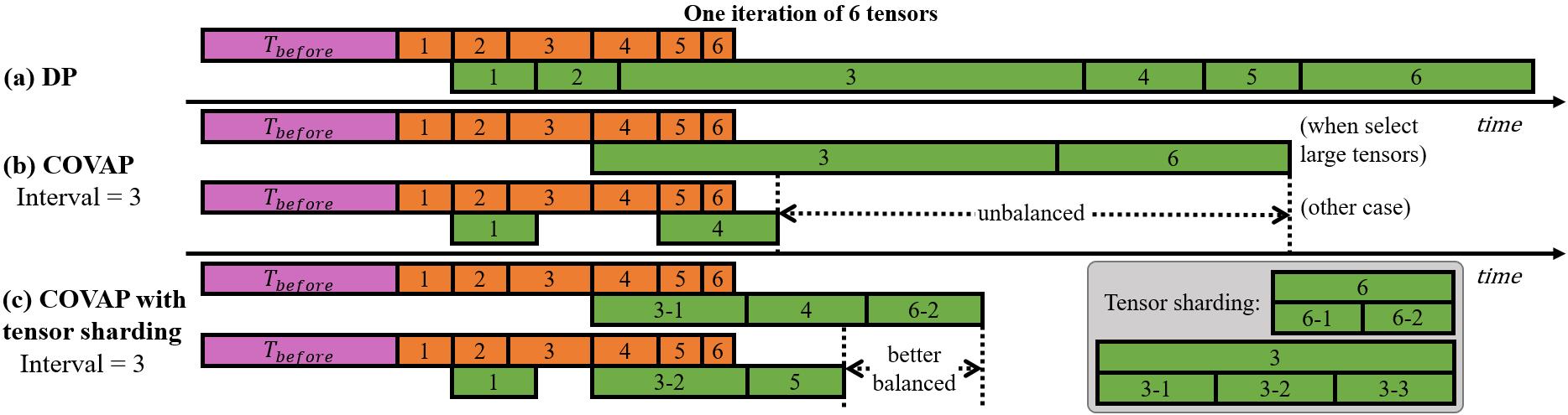
In such coarse-grained filter, the tensor selection strategy is also different from other GC schemes. In each iteration, each worker chooses tensors with same index to communicate with others. Tensors are selected alternately, which means each tensor is only communicated once in every iterations ( represents the interval). Meanwhile, only one tensor is chosen for communication from every tensors in each iteration. Tensor is selected in iteration when . Fig. 2(a) illustrates the above selection strategy. When the interval is 4, the first tensor is communicated at the first and iterations, the second tensor is communicated at the second and iterations, and so on. One benefit of such a strategy is that each tensor is communicated and updated by the same interval, which can alleviate the negative effect of staleness [30] on training convergence. Another benefit is that it does not introduce any additional data dependencies mentioned in Section I because each worker can select tensors by themselves according to the current iteration numbers and the interval (The interval is determined in the early stage of training and remains unchanged in subsequent training, we give a detailed discussion in section III.B.), which means no additional communication is required to synchronize the tensor selection results.

III-B Compression ratio selection
The coarse-grained filter has minimized compression overhead. However, for various training tasks in different computing environments, a constant compression ratio is difficult to achieve fully overlapping consistently. In other words, s are different in different cases. For example, using different GPU types can significantly influence the : replacing the GPU from V100 to A100 will speed up the computation and increase . Therefore, to achieve full overlapping in most cases, COVAP adopts different compression ratios for different cases. Note that in this paper, we do not consider the interference from other tasks in the cluster or other performance fluctuations, which means will not change rapidly throughout whole training.
From the analysis in Section II.D, COVAP should decrease communication time by times. Since COVAP uses the same collective communication primitives (i.e., AllReduce) as the baseline of no compression, decreasing communication overhead by times is equivalent to reducing communication data volume by times. Because communication tensors of DL frameworks are generally in fixed sizes [14, 20], COVAP initially assumes each tensor has the same size. Then, reducing data volume by times can be approximated as reducing the number of communicating tensors by times. We can infer from the algorithm in Section III.A that the interval in our scheme should equal .
COVAP measures the in the early stage of the training task and sets its compression ratio according to the result. For implementation details, COVAP measures the s of different DNNs based on the PyTorch profiler module. PyTorch profiler’s context manager API can be used to study device kernel activity and visualize the execution trace. Specifically, we use the profiler_cuda module to track cuda events, including communication (i.e., AllReduce and AllGather) and computation (i.e., forward and backward propagation) operators. Since we only need to profile one training iteration to obtain the communication and computation time, COVAP only costs a one-off profiling overhead (less than 5 seconds in our experiments). Compared to hours of training, such profiling overhead is acceptable.
The profiler tool provided by PyTorch is applicable for stand-alone programs. In distributed training, PyTorch creates multi-processes for different workers. Although we can use the original profiler to monitor one of the processes and obtain its exact time of computation events in one iteration, the communication time measured in this way may be inaccurate. That is because there may be a slight time difference in distributed training when different workers start their communications on different nodes, as Fig. 3 shows. In such cases, the communication operators of some workers who finish their computations early will be longer than others since they must wait for other workers to rendezvous in communication. In our experiments, such waiting may cause a 20% communication time measurement error. Therefore, we develop a distributed profiler. The key point is to align the timeline at the end of each communication operator in each training step to eliminate measurement errors caused by such communication waiting latency.
Using that distributed profiler, we can obtain more accurate communication time to compute . Then, COVAP sets the interval of the filter according to that . Since must be an integer but measured s may not be integers, we let equals to , which implies that COVAP compresses communication by a little more than times to ensure as much communication as possible can be overlapped with computation in DP.
III-C Tensor Sharding
In Section III.B, we assumed that each communication tensor has the same size as the default fixed size of DL frameworks. However, the practical tensor sizes may vary significantly according to severe imbalanced sizes of DNN layers, which could cause communication bottlenecks if the large tensors are selected to communicate in COVAP. In practice, DL frameworks allocate gradients of layers into tensors. The gradient tensor of one layer is used as the minimum unit in allocations, which means each tensor contains integral number of layers and at least one. Even if a layer’s size is much larger than the tensor size of the framework, PyTorch will not split such a large variable into multiple tensors. Although DL frameworks often adopt a much larger default tensor size than the size of most layers in DNNs, there may still exist some much larger layers than the default tensor size in some DNNs. For example, we list some of the layers of VGG-19 in Table IV. It can be seen that the parameter number of Layer FC1 is much larger than other layers, accounting for 71.53% of all parameters. The size of Layer FC1 is 102760448 * 4 Bytes = 401.4 MB. Compared with the default tensor size of 25MB in PyTorch DDP, the tensor of that layer is oversized. We also tested the communication time of all tensors when training VGG-19 across 8 nodes, and the result is shown in Table V. The communication of that large tensor costs about 603.238ms, accounting for 72.67% of total communication time. Such prominent communications of large layers may impair the Overlapping advantage in COVAP due to the imbalance, as shown in Fig. 4(b).
| Layer name | parameters | ratio |
| Input | — | — |
| Conv1_1 | 1728 | 0.00% |
| Conv1_2 | 36864 | 0.03% |
| Pool1 | — | — |
| …… | ||
| Pool5 | — | — |
| FC3 | 4096000 | 2.85% |
| Softmax | — | — |
| total | 143652544 | 100.00% |
| Tensor id | Number of elements | comunication time | ratio |
|---|---|---|---|
| 1 | 4101096 | 16.177ms | 1.95% |
| 4 | 7079424 | 36.513ms | 4.40% |
| 5 | 7669760 | 40.743ms | 4.91% |
| 6 | 555072 | 34.218ms | 4.12% |
| total | 143667240 | 830.094ms | 100.00% |
Therefore, COVAP designs a tensor sharding strategy that slices the large tensor into small pieces such that all tensors are balanced in size. Specifically, after building tensors, COVAP counts the elements’ number of all tensors to find the median number of elements in one tensor. Suppose a tensor has multiple times elements than that median number. In that case, COVAP evenly slices it into parts, where represents the elements’ number of that tensor (i.e., the total number of gradients of all layers in that tensor). Note that if is larger than interval , COVAP only slices that tensor into parts for balance.
Then, when COVAP selects tensors to communicate, such a large tensor is regarded as tensors, from which COVAP may choose one tensor to communicate in one iteration. Still using VGG-19 as an example, as shown in Table V, the median element number of tensors is 5590260. Thus, the second and third tensors are sliced into 3 and 19 new tensors (if the interval is less than 3 or 19, COVAP slices them into parts instead). Then, the total number of tensors is regarded as 26 when COVAP chooses tensors for communication, which results in a much better balance of tensor sizes. Another example of how COVAP selects tensors when using tensor sharding is shown in Fig. 2(b), and how tensor sharding balances the communication time is shown in Fig. 4(c).
III-D Convergence
. Although COVAP significantly improves training speed with techniques in Section III.A, III.B and III.C, such compression schemes are theoretically lossy in training accuracy. To alleviate such a problem, COVAP equips error feedback (i.e., local memory accumulation) to ensure convergence and designs a new scheduler to continuously adjust a compensation coefficient of Error feedback in training, which balances the feedback amount of errors.
| Error feedback in compression given gradient . | ||
| 1: | ||
| 2: | += | |
| 3: | = sparsification_or_quantization() | |
| 4: | = - | |
| 5: | return | |
| 6: | ||
The idea of error feedback was first introduced in one-bit [19]. Following GC works [3, 7, 11, 13, 16, 24, 26] widely adopted error feedback as a compensation strategy to ensure convergence and preserve accuracy. Several works [23, 24] also conducted theoretical analyses. Generally, error feedback is used as shown in Algorithm 1, where represent the D-values saved in local memory.
In COVAP, we only choose a few tensors to communicate in each iteration. Applying error feedback to COVAP means we save other tensors’ gradients in local memory and add them to their corresponding tensor in the next iteration, just like Algorithm 1. However, in practice, we found that using error feedback in such a way may lead to divergence due to the harmful effect of the staleness of delayed update parameters. To alleviate the staleness effect, we introduce the error feedback scheduler into Algorithm 1 based on the observation in [10] that a large compensation coefficient in early training epochs may harm model accuracy.
The error feedback scheduler multiplies residuals by a compensation coefficient before the residuals are added to current gradients (i.e., line 2 in Algorithm 1). Similar to the learning rate scheduler of variant declining strategies, our scheduler adjusts that coefficient continuously with increasing strategy in training. The coefficient is equal to:
where represents the initial value of the coefficient, represents the number of iterations trained, represents the interval between ascending, and represents the ascending range. The max value of the coefficient is 1.
. From Section III.A, the filter of COVAP is similar to sparsification schemes since COVAP also selects a subset of all gradients in each iteration. Similar to Top-k[3], COVAP can be regarded as a particular case of Random-k [23]. Therefore, we can follow the theoretical proof in [23].
We first give the definition of COVAP’s compression operator:
IV Evaluation
IV-A Experimental setup


We conducted our experiments on 8 Alibaba Cloud ECS instances. Each instance contains an Intel Xeon Platinum 8163 CPU and 8 NVIDIA V100 GPUs with 16 GB global memory. We choose a typical bandwidth of 30Gbps in the public cloud. In High-Performance Computing, the bandwidth is usually much higher and reaches 100Gbps. Due to the adaptive compression ratio relying on , we believe COVAP can also provide acceleration in such scenarios.
| Task | DNN | parameters | datasets |
|---|---|---|---|
| Image classification | ResNet-101 | 44654504 | Cifar-10/ImageNet |
| VGG-19 | 143652544 | ||
| Text classification | Bert | 102267648 | THUC-News |
| Text generation | GPT-2 | 81894144 |
| GC schemes | ResNet-101 | VGG-19 | Bert | GPT-2 | |||||||||||
|---|---|---|---|---|---|---|---|---|---|---|---|---|---|---|---|
| time(s) | accuracy(%) | speedup | time(s) | accuracy(%) | speedup | time(s) | accuracy(%) | speedup | time(s) | loss | speedup | ||||
| DDPovlp | 31260.4 | 74.626 | 21.52 | 56201.9 | 66.068 | 12.07 | 729.8 | 94.58 | 26.64 | 28296.9 | 1.922 | 19.10 | |||
| Top-k | 64158.6 | 35.424 | 10.48 | 192920.2 | 55.804 | 3.51 | 1271.4 | 94.46 | 15.28 | 47570.6 | 2.697 | 11.366 | |||
| DGC | 40516.6 | 50.14 | 16.64 | 115819.0 | 57.006 | 5.85 | 431.2 | 94.33 | 45.12 | 43772.2 | 1.953 | 12.35 | |||
| EFsignSGD | 179978.9 | 73.532 | 3.76 | 255388.2 | 28.482 | 2.66 | 978.5 | 93.88 | 19.92 | 192404.4 | 1.974 | 2.81 | |||
| FP16 | 21312.3 | 74.68 | 31.6 | 36293.4 | 66.248 | 18.68 | 473 | 94.38 | 41.12 | 16167.6 | 1.945 | 33.44 | |||
| PowerSGD | 22485.2 | 71.916 | 29.92 | 20320.5 | 61.544 | 33.37 | 428.9 | 93.98 | 45.36 | 10844.9 | 2.253 | 49.85 | |||
| Ok-topk | 26292.6 | 61.022 | 25.6 | 74646.3 | 57.018 | 9.08 | 609.6 | 93.97 | 31.92 | 15390.2 | 2.061 | 35.13 | |||
| COVAP | 11696.9 | 74.633 | 57.52 | 13090.4 | 66.633 | 51.80 | 336.4 | 94.44 | 57.84 | 9635.4 | 1.937 | 56.11 | |||
We use four neural networks from different deep learning domains summarized in Table VI for evaluation. For VGG-19 and ResNet-101, we use SGD optimizer with an initial learning rate of 1e-3; for Bert and GPT-2, we use Adam optimizer with initial an learning rate of 5e-5 and 1.5e-4. We compare our scheme COVAP with the state-of-the-art and other popular GC schemes in Table II. For a fair comparison, all schemes are implemented by the DDP communication hook in PyTorch 1.9.0 using NCCL as the communication library.
IV-B Compression ratio selection
We verify the correctness of the adaptive compression ratio selection strategy introduced in Section III.B on three different DNNs. Fig. 5 shows the performance of COVAP in using different compression ratios. We tested the speedups provided by COVAP in all cases. The speedups were calculated by (1) and (2) such that the upper limit speedup of DP training with 64 GPUs is 64, as dotted lines shown in Fig. 5. Compression ratio 1 represents the baseline without compression (i.e., default PyTorch DDP).
As discussed in Section III.B, COVAP chooses as its compression ratio. Using a higher compression ratio than is meaningless because COVAP has already reduced most communication overhead through Overlapping. In Fig. 5(a), the speedup of training ResNet-101 increased very slowly as the compression ratio was beyond 3. Similarly, Fig. 5(b) and 5(c) discover the maximum speedups were 51.51 and 54.55 when the compression ratio was 4, which COVAP selected.
IV-C Case studies on training time and convergence
We studied the training time and model convergence using real-world applications listed in Table VI. In addition to listing the results of each complete training, we make a further breakdown of the training time of one iteration for better understanding, including compression (e.g., Top-k selection from the gradients), communication (e.g., AllReduce), and computation (i.e., forward and backward pass). The experiments were conducted in an 8-node cluster with a 30Gbps network, each node with 8 NVIDIA V100 GPUs. Note that we use average values for breakdowns since some GC schemes’ training speed varies significantly at different stages of training. For linear scaling, the speedup should be 64 (compared with one GPU), which is also an upper limit of all schemes. Besides, since Random-k diverged in most experiments, we do not give the convergence result of Random-k. Table VII presents the training time and accuracy results of different GC schemes when training 4 DNNs, wherein the speedup is calculated by (2) in Section II.A. Fig. 6 presents the time-to-solution curves of 3 DNNs except for Bert, since we only use the title of each news in THUC-News for text classification and its training time is relatively short. DDPovlp represents the default PyTorch with Overlapping and is the baseline with no gradient compression.


IV-C1 ResNet-101
Fig. 7 shows the breakdown of each iteration’s training time of different GC schemes when training ResNet-101 on ImageNet. ’ represents communication overhead that cannot be overlapped with computation. Although Top-k hid almost all communication overhead (’), it had a considerable compression overhead of about 370ms, which resulted in 2.05x longer training time than the baseline. Besides, since some schemes use synchronized communications, they are incompatible with Overlapping. One example is Ok-topk. Although it has a lower compression overhead of about 40ms than 370ms of Top-k, its communication cannot be overlapped with computation, so its training speed only exceeded the baseline by 1.19x. Another example is PowerSGD. Although it had the lowest communication overhead of 20ms and low compression overhead of 10ms, its performance did not outperform COVAP and FP16. From Table VII and Fig. 6(a), COVAP achieved the best performance among all GC schemes, outperformed the others by 1.92x-15.39x for the total training time and achieved linear scaling. For model convergence, only 3 GC schemes achieved similar accuracy as the baseline, and all sparsification schemes (including Top-k, DGC, and Ok-topk) did not reach the desired accuracy.
IV-C2 VGG-19
Fig. 8 shows the breakdown of VGG-19 training time. Notably, ResNet-101 had a lower of 2.1 compared to VGG-19’s of 4.0 due to the larger parameter amount of VGG-19, which implies training VGG-19 has more severe communication bottleneck so that the baseline DDPovlp had lower speedups from 21.52x on ResNet-101 to 12.07x on VGG-19. In such a case, the speedup of FP16 is only 18.68x compared to 31.6x on ResNet-101 due to insufficient compression. Besides, only COVAP did not suffer from 2x-6.67x larger compression overhead, which benefited from the low time complexity of our coarse-grained filter. Moreover, COVAP adaptively selected its compression ratio to 4 according to the higher of VGG-19. In VGG-19 training, COVAP outperformed all other schemes by 1.55x-19.51x in training time.
Fig. 6(b) shows the time-to-solution curves of different GC schemes when training VGG-19. For convergence, only COVAP and FP16 achieved similar accuracy as the baseline. It is noteworthy that some GC scheme has better (e.g., sparsification) or worse (e.g., EfsignSGD) accuracy when training VGG-19 compared with training ResNet-101, which indicates that those GC schemes may only guarantee convergence and accuracy on specific DNNs.


IV-C3 Bert
Fig. 9 shows the breakdown of Bert training time. Similar to the experiments on ResNet-101 and VGG-19, COVAP had a better performance than all counterparts, outperforming them by 1.27x-3.78x in training time. Regarding model convergence, the accuracy achieved by COVAP was 0.14% lower than the baseline. Among all schemes, COVAP achieved the fastest time-to-solution and near-linear scaling in 9.6% less speedup than the optimal case.
IV-C4 GPT-2
Fig. 10 shows the breakdown of GPT-2 training time. The of GPT-2 measured by our distributed profiler is about 3.5, so we set the compression ratio to 4. Fig. 6(c) shows time-to-solution of all GC schemes. Unlike CV tasks, only Top-k had apparent lower accuracy than the baseline. In GPT-2 training, COVAP outperformed all other schemes by 1.13x-19.96x in training time while achieving expected accuracy.
IV-D Scalability
We compared COVAP’s scalability with other GC schemes using 3 DNNs. The experiments were conducted on four clusters of 8, 16, 32 and 64 GPUs. Since we did not need to focus on training accuracy here, we used Cifar-10 as the dataset for ResNet-101 and VGG-19. The result is shown in Fig. 11, where the linear scaling bar represents the upper limit speedup of DP.
Fig. 11(a) shows that COVAP obtained speedups of only 5% less than linear scaling under four different clusters in ResNet-101 training, compared with 30% less of PowerSGD. Besides, AllReduce-based GC schemes showed no degradation as the cluster size increased since AllReduce has better scalability than AllGather. For example, AllGather-based Random-k and EFsignSGD obtained only 3.2x acceleration while the GPU number increased by 8x. COVAP scaled even better than other AllReduce-based schemes because it essentially reduced the number of communication operations in each iteration. Another reason is that COVAP adjusted its compression ratio adaptively according to the change of while other GC schemes kept their compression ratios (or other hyperparameters) unchanged. Specifically, COVAP outperformed other schemes by 1.15x-9.03x on 64 GPUs, compared with 1.04x-3.02x on 8 GPUs.
Fig. 11(b) and Fig. 11(c) show the scalabilities of all schemes in training VGG-19 and Bert. Note that we could not scale Top-k, Random-k, DGC, EFsignSGD, and Ok-topk beyond 16 GPUs in training VGG-19 since AllGather requires more memory than AllReduce when cluster scaled and caused running out of memory. The comparison of Fig. 11(a) and 11(b) disclosed that the 3x longer communication overhead of VGG-19 than ResNet-101 degraded its scalabilities of all schemes, while COVAP preserved the best stability in all cases along with cluster scaling.
V Limitations
The compression ratio of COVAP correlates intensely to the of DNN training. As shown in Table I, the of DNNs at a common network of 30-100 Gbps bandwidth is generally not too high (i.e., <5). However, in worse network cases such as federated learning or edge computing, the would be much higher, whereas the sparsification schemes using a high compression ratio work well. In such cases, an exorbitant compression ratio of COVAP may lead to an accuracy decline because of worse staleness [30]. One of our future works is to handle this issue.
VI Related works
. Many GC schemes [16, 17, 22, 29] are proposed for poor network environments (e.g., <10Gbps bandwidth) where the communication bottleneck is particularly severe. Therefore, those works often focus on enlarging their compression ratios to reduce communication overhead as much as possible. In addition, several GC schemes [6, 15, 27] were proposed to improve security and privacy in federated learning since private information can be leaked through shared gradients.
| Technique | Forward Pass | Gradient computation | communication |
|---|---|---|---|
| LayerDrop | discarded | discarded | discarded |
| Freeze training | reserved | discarded | discarded |
| COVAP | reserved | reserved | discarded |
. Fan [9] proposed a form of structured dropout called LayerDrop, which selects and drops several layers of DNN in training. The motivation of LayerDrop is to regularize very deep Transformers while stabilizing its training. It also makes the network robust to subsequent pruning. Freeze Training is a helpful technique widely adopted in the object detection field. Since some parts of pre-training weights are universal, such as the backbone, we do not need to compute the gradients and update the weights of those layers. In PyTorch, it is easy to use Freeze Training by setting the of those layers to False.
Similar to these two techniques, COVAP also discards some stages of DP (Note that these two techniques are not GC schemes). Table VIII shows their difference. Besides the difference in discarded stages, COVAP adopts a different discard granularity: Tensor, instead of layer in LayerDrop and Freeze training.
VII Conclusion
COVAP is a novel gradient compression scheme combining Overlapping for distributed data parallel deep learning training. COVAP adaptively reduces the communication overhead approach to the computation time, making the communication almost fully hidden while introducing close-to-zero compression overhead. Empirical results for data parallel training of real-world deep learning models on Alibaba Cloud ECS instances show that COVAP achieves near-linear scaling in all experiments and significantly improves the training speed by up to 15.39x than existent gradient compression schemes while reaching similar model accuracy to the baseline.
Acknowledgment
This work is supported in part by Science and Technology Innovation 2030 - Major Project (No. 2022ZD0119104). The opinions, findings and conclusions expressed in this paper are those of the authors and do not necessarily reflect the views of the funding agencies or the government.
References
- [1] Abadi M, Barham P, Chen J, et al. TensorFlow: a system for Large-Scale machine learning[C]//12th USENIX symposium on operating systems design and implementation (OSDI 16). 2016: 265-283.
- [2] Agarwal, S., Wang, H., Venkataraman, S., & Papailiopoulos, D. (2022). On the utility of gradient compression in distributed training systems. Proceedings of Machine Learning and Systems, 4, 652-672.
- [3] Aji, A., & Heafield, K. (2017, September). Sparse Communication for Distributed Gradient Descent. In EMNLP 2017: Conference on Empirical Methods in Natural Language Processing (pp. 440-445). Association for Computational Linguistics (ACL).
- [4] Bai, Y., Li, C., Zhou, Q., Yi, J., Gong, P., Yan, F., … & Xu, Y. (2021, October). Gradient compression supercharged high-performance data parallel dnn training. In Proceedings of the ACM SIGOPS 28th Symposium on Operating Systems Principles (pp. 359-375).
- [5] Chahal, K. S., Grover, M. S., Dey, K., & Shah, R. R. (2020). A hitchhiker’s guide on distributed training of deep neural networks. Journal of Parallel and Distributed Computing, 137, 65-76.
- [6] Chaudhuri, K., Guo, C., & Rabbat, M. (2022, August). Privacy-aware compression for federated data analysis. In Uncertainty in Artificial Intelligence (pp. 296-306). PMLR.
- [7] Chen, C. Y., Choi, J., Brand, D., Agrawal, A., Zhang, W., & Gopalakrishnan, K. (2018, April). Adacomp: Adaptive residual gradient compression for data-parallel distributed training. In Proceedings of the AAAI conference on artificial intelligence (Vol. 32, No. 1).
- [8] Dean, J., Corrado, G., Monga, R., Chen, K., Devin, M., Mao, M., … & Ng, A. (2012). Large scale distributed deep networks. Advances in neural information processing systems, 25.
- [9] Fan, A., Grave, E., & Joulin, A. (2019, September). Reducing Transformer Depth on Demand with Structured Dropout. In International Conference on Learning Representations.
- [10] Hong, Y., & Han, P. (2021). LSDDL: Layer-wise sparsification for distributed deep learning. Big Data Research, 26, 100272.
- [11] Karimireddy, S. P., Rebjock, Q., Stich, S., & Jaggi, M. (2019, May). Error feedback fixes signsgd and other gradient compression schemes. In International Conference on Machine Learning (pp. 3252-3261). PMLR.
- [12] Ko, Y., Choi, K., Seo, J., & Kim, S. W. (2021, May). An in-depth analysis of distributed training of deep neural networks. In 2021 IEEE International Parallel and Distributed Processing Symposium (IPDPS) (pp. 994-1003). IEEE.
- [13] Li, S., & Hoefler, T. (2022, April). Near-optimal sparse allreduce for distributed deep learning. In Proceedings of the 27th ACM SIGPLAN Symposium on Principles and Practice of Parallel Programming (pp. 135-149).
- [14] Li, S., Zhao, Y., Varma, R., Salpekar, O., Noordhuis, P., Li, T., … & Chintala, S. PyTorch Distributed: Experiences on Accelerating Data Parallel Training. Proceedings of the VLDB Endowment, 13(12).
- [15] Li, Z., Zhang, J., Liu, L., & Liu, J. (2022). Auditing privacy defenses in federated learning via generative gradient leakage. In Proceedings of the IEEE/CVF Conference on Computer Vision and Pattern Recognition (pp. 10132-10142).
- [16] Lin, Y., Han, S., Mao, H., Wang, Y., & Dally, B. (2018, February). Deep Gradient Compression: Reducing the Communication Bandwidth for Distributed Training. In International Conference on Learning Representations.
- [17] Liu, P., Jiang, J., Zhu, G., Cheng, L., Jiang, W., Luo, W., … & Wang, Z. (2022, April). Training time minimization in quantized federated edge learning under bandwidth constraint. In 2022 IEEE Wireless Communications and Networking Conference (WCNC) (pp. 530-535). IEEE.
- [18] Paszke, A., Gross, S., Massa, F., Lerer, A., Bradbury, J., Chanan, G., … & Chintala, S. (2019). Pytorch: An imperative style, high-performance deep learning library. Advances in neural information processing systems, 32.
- [19] Seide, F., Fu, H., Droppo, J., Li, G., & Yu, D. (2014). 1-bit stochastic gradient descent and its application to data-parallel distributed training of speech dnns. In Fifteenth annual conference of the international speech communication association.
- [20] Sergeev, A., & Del Balso, M. (2018). Horovod: fast and easy distributed deep learning in TensorFlow. arXiv preprint arXiv:1802.05799.
- [21] Shi, S., Chu, X., & Li, B. (2019, April). MG-WFBP: Efficient data communication for distributed synchronous SGD algorithms. In IEEE INFOCOM 2019-IEEE Conference on Computer Communications (pp. 172-180). IEEE.
- [22] Shi, S., Wang, Q., Zhao, K., Tang, Z., Wang, Y., Huang, X., & Chu, X. (2019, July). A distributed synchronous SGD algorithm with global top-k sparsification for low bandwidth networks. In 2019 IEEE 39th International Conference on Distributed Computing Systems (ICDCS) (pp. 2238-2247). IEEE.
- [23] Stich, S. U., Cordonnier, J. B., & Jaggi, M. (2018). Sparsified SGD with memory. Advances in Neural Information Processing Systems, 31.
- [24] Stich, S. U., & Karimireddy, S. P. (2020). The error-feedback framework: Better rates for sgd with delayed gradients and compressed updates. The Journal of Machine Learning Research, 21(1), 9613-9648.
- [25] Ström, N. (2015). Scalable distributed DNN training using commodity GPU cloud computing.
- [26] Vogels, T., Karimireddy, S. P., & Jaggi, M. (2019). PowerSGD: Practical low-rank gradient compression for distributed optimization. Advances in Neural Information Processing Systems, 32.
- [27] Wu, C., Wu, F., Lyu, L., Huang, Y., & Xie, X. (2022). Communication-efficient federated learning via knowledge distillation. Nature communications, 13(1), 2032.
- [28] Xu, H., Ho, C. Y., Abdelmoniem, A. M., Dutta, A., Bergou, E. H., Karatsenidis, K., … & Kalnis, P. (2021, July). GRACE: A compressed communication framework for distributed machine learning. In 2021 IEEE 41st international conference on distributed computing systems (ICDCS) (pp. 561-572). IEEE.
- [29] Yan, M., Meisburger, N., Medini, T., & Shrivastava, A. (2022). Distributed slide: Enabling training large neural networks on low bandwidth and simple cpu-clusters via model parallelism and sparsity. arXiv preprint arXiv:2201.12667.
- [30] Zhang, W., Gupta, S., Lian, X., & Liu, J. (2016, July). Staleness-Aware Async-SGD for distributed deep learning. In International Joint Conference on Artificial Intelligence. International Joint Conferences on Artificial Intelligence.