MVIN: Learning Multiview Items for Recommendation
Abstract.
Researchers have begun to utilize heterogeneous knowledge graphs (KGs) as auxiliary information in recommendation systems to mitigate the cold start and sparsity issues. However, utilizing a graph neural network (GNN) to capture information in KG and further apply in RS is still problematic as it is unable to see each item’s properties from multiple perspectives. To address these issues, we propose the multi-view item network (MVIN), a GNN-based recommendation model which provides superior recommendations by describing items from a unique mixed view from user and entity angles. MVIN learns item representations from both the user view and the entity view. From the user view, user-oriented modules score and aggregate features to make recommendations from a personalized perspective constructed according to KG entities which incorporates user click information. From the entity view, the mixing layer contrasts layer-wise GCN information to further obtain comprehensive features from internal entity-entity interactions in the KG. We evaluate MVIN on three real-world datasets: MovieLens-1M (ML-1M), LFM-1b 2015 (LFM-1b), and Amazon-Book (AZ-book). Results show that MVIN significantly outperforms state-of-the-art methods on these three datasets. In addition, from user-view cases, we find that MVIN indeed captures entities that attract users. Figures further illustrate that mixing layers in a heterogeneous KG plays a vital role in neighborhood information aggregation.
1. Introduction
Recommendation systems (RSs), like many other practical applications with extensive learning data, have benefited greatly from deep neural networks. Collaborative filtering (CF) with matrix factorization (Koren et al., 2009) is arguably one of the most successful methods for recommendation in various commercial fields (Oh et al., 2014). However, CF-based methods’ reliance on past interaction between users and items leads to the cold-start problem (Schein et al., 2002), in which items with no interaction are never recommended. To mitigate this, researchers have experimented with incorporating auxiliary information such as social networks (Jamali and Ester, 2010), images (Zhang et al., 2016a), and reviews (Zheng et al., 2017).
Among the many types of auxiliary information, knowledge graphs111A knowledge graph is typically described as consisting of entity-relation-entity triplets, where the entity can be an item or an attribute., denoted as KGs hereafter, have widely been used since they can include rich information in the form of machine-readable entity-relation-entity triplets. Researchers have successively utilized KGs in applications such as node classification (Hamilton et al., 2017), sentence completion (Koncel-Kedziorski et al., 2019), and summary generation (Li et al., 2019). In view of the success of KGs in a wide variety of tasks, researchers have developed KG-aware recommendation models, many of which have benefited from graph neural networks (GNNs) (Wang et al., 2018b; Wang et al., 2019d; Wang et al., 2019c; Wang et al., 2019a; Wu et al., 2019; Wang et al., 2019b; Xin et al., 2019) which capture high-order structure in graphs and refine the embeddings of users and items. For example, RippleNet (Wang et al., 2018b) propagates users’ potential preferences in the KG and explores their hierarchical interests. Wang et al. (Wang et al., 2019d) employ an KG graph convolutional network (GCN) (Kipf and Welling, 2016), which is incorporated in a GNN to generate high-order item connectivity features. However, in these models, items look identical to all users (Wang et al., 2018b; Wang et al., 2019a; Xin et al., 2019), and using GCN with KGs still has drawbacks such as missing comparisons between entities of different layers (Abu-El-Haija et al., 2019).
We further give some examples that explain the user view and the entity view. Imagine some users are interested in books of the same author, and other users are interested in a certain book genre, where authorship and genre are two relations between the book and its neighborhood (author, genre type) in the knowledge base. We can say that in the real world every user has a different view of a given item. In the entity-view, item representations are defined by the entities connected to it in the KG. A sophisticated representation can be generated by incorporating smart operations of entities. For example, this paper refines it by leveraging the layer-wise entity difference to keep information from neighborhood entities. To illustrate the need for this difference feature, imagine that we seek to emphasize a new actor in a movie directed by a famous director, contrasting entities related to the famous director at the second layer to the director at the first layer will have stronger expressiveness than aggregating all of the directors he has co-worked with back him.
Overall, there are still challenges with GNN-based recommendation models: (1) user-view GNN enrichment and (2) entity-view GCN refinement. In this paper, we investigate GNN-based recommendation and propose a network that meets the above challenges. We propose a knowledge graph multi-view item network (MVIN), a GNN-based recommendation model equipped with user-entity and entity-entity interaction modules. To enrich user-entity interaction, we first learn the KG-enhanced user representations, using which the user-oriented modules characterize the importance of relations and informativeness for each entity. To refine the entity-entity interaction, we propose a mixing layer to further improve embeddings of entities aggregated by GCN and allow MVIN to capture the mixed GCN information from the various layer-wise neighborhood features. Furthermore, to maintain computational efficiency and approach the panoramic view of the whole neighborhood, we adopt a stage-wise strategy (Barshan and Fieguth, 2015) and sampling strategy (Wang et al., 2019d; Ying et al., 2018) to better utilize KG information.
We evaluate MVIN performance on three real-world datasets: ML-1M, LFM-1b, and AZ-book. For click-through rate (CTR) prediction and top- recommendation, MVIN significantly outperforms state-of-the-art models. Through ablation studies, we further verify the effectiveness of each component in MVIN and show that the mixing layer plays a vital role in both homogeneous and heterogeneous graphs with a large neighborhood sampling size. Our contributions include:
-
•
We enable the user view and personalize the GNN.
-
•
We refine item embeddings from the entity view by a wide and deep GCN which brings in layer-wise differences to high-order connectivity.
-
•
We conduct experiments on three real-world datasets with KGs of different sizes to show the robustness and superiority of MVIN.222We release the codes and datasets at https://github.com/johnnyjana730/MVIN/ In addition, we demonstrate that MVIN captures entities which identify user interests, and that layer-wise differences are vital with large neighborhood sampling sizes in heterogeneous KGs.
2. Related Work
For recommendation, there are other models that leverage KGs, and there are other models that consider interaction between users and items. We introduce these below.
2.1. KG-aware Recommendation Models
In addition to graph neural network (GNN) based methods, there are two other categories of KG-aware recommendation.
The first is embedding-based methods (Cao et al., 2019b; Huang et al., 2018; Zhang et al., 2016b; Wang et al., 2018c; Cao et al., 2019a; Zhang et al., 2018), which combine entities and relations of a KG into continuous vector spaces and then aid the recommendation system by enhancing the semantic representation. For example, DKN (Wang et al., 2018) fuses semantic-level and knowledge-level representations of news and incorporates KG representation into news recommendation. In addition, CKE (Zhang et al., 2016a) combines a CF module with structural, textual, and visual knowledge into a unified recommendation framework. However, these embedding-based knowledge graph embedding (KGE) algorithms methods are more suitable for in-graph applications such as link prediction or KG completion rather than for recommendation (Wang et al., 2017). Nevertheless, we still select (Zhang et al., 2016a) for comparison.
The second category is path-based methods (Hu et al., 2018b; Sun et al., 2018; Wang et al., 2018a; Yu et al., 2014; Zhao et al., 2017), which utilize meta paths and related user-item pairs, exploring patterns of connections among items in a KG. For instance, MCRec (Hu et al., 2018b) learns an explicit representation for meta paths in recommendation. In addition, it considers the mutual effect between the meta path and user-item pairs. Compared to embedding-based methods, path-based methods use the graph algorithm directly to exploit the KG structure more naturally and intuitively. However, they rely heavily on meta paths, which require domain knowledge and manual labor to process, and are therefore poorly suited to end-to-end training (Wang et al., 2018b). We also provide the performance of the state-of-the-art path-based model (Hu et al., 2018b) as a baseline for comparison.
2.2. User-Item Interaction
As users and items are two major entities involved in recommendation, many works attempt to improve recommendation performance by studying user-item interaction.
For example, as a KG-aware recommendation model, Wang et al. (Wang et al., 2019d) propose KGCN, which characterizes the importance of the relationship to the user. However, the aggregation method in KGCN does not consider the informativeness of entities different from the user. Hu et al. (Hu et al., 2018a) propose MCRec, which considers users’ different preferences over the meta paths. Nevertheless, it neglects semantic differences of relations to users. Also, they do not employ GCN and thus information on high-order connectivity is limited.
With their KG-free recommendation model, Wu et al. (Wu et al., 2019) consider that as the informativeness of a given word may differ between users, they propose NPA, which uses the user ID embedding as the query vector to differentially attend to important words and news according to user preferences. An et al. (An et al., 2019) consider that users typically have both long-term preferences and short-term interests, and propose LSTUR which adds user representation into the GRU to capture the user’s individual long- and short-term interests.
3. Recommendation Task Formulation
Here we clarify terminology used here and explicitly formulate MVIN, the proposed GNN-based recommendation model.
In a typical recommendation scenario, the sets of users and items are denoted as and , and the user-item interaction matrix is defined according to implicit user feedback. If there is an observed interaction between user and item , is recorded as ; otherwise . In addition, to enhance recommendation quality, we leverage the information in the knowledge graph , which is comprised of entity-relation-entity triplets . Triplet describes relations from head entity to tail entity , and and denote the set of entities and relations in . Moreover, an item may be associated with one or more entities in ; refers to these neighboring entities around . Given interaction matrix and knowledge graph , we seek to predict whether user has a potential interest in item . The ultimate goal is to learn the prediction function , where is the probability that user engages with item , and stands for the model parameters of function .
4. MVIN

We describe in detail MVIN, the proposed recommendation model, shown in Figure 1, which enhances item representations through user-entity interaction, which describes how MVIN collects KG entities information from a user perspective, and entity-entity interaction, which helps MVIN not only to aggregate high-order connectivity information but also to mix layer-wise GCN information.
4.1. User-Entity Interaction
To improve the user-oriented performance, we split user-entity interaction into user-oriented relation attention, user-oriented entity projection, and KG-enhanced user representation.
4.1.1. User-Oriented Relation Attention
When MVIN collects information from the neighborhood of the given item in the KG, it scores each relation around the item in a user-specific way. The proposed user-oriented relation attention mechanism utilizes the information of the given user, item, and relations to determine which neighbor connected to the item is more informative. For instance, some users may think the film Iron Man is famous for its main actor Robert Downey Jr.; others may think the film Life of Pi is famous for its director Ang Lee. Thus each entity of neighborhood is weighted by dependent scores , where denotes a different user; denotes the relation from entity to neighboring entity (the formulation of the scoring method is given below). We aggregate the weighted neighboring entity embeddings and generate the final user-oriented neighborhood information n as
| (1) | n | |||
| (2) |
To calculate the neighbor’s dependent score , we first concatenate relation , item representation , and user embedding , and then transform these to generate the final user-oriented score as
| (3) |
where and are trainable parameters.
4.1.2. User-Oriented Entity Projection
To further increase user-entity interaction, we propose a user-oriented entity projection module. For different users, KG entities should have different informativeness to characterize their properties. For instance, in a movie recommendation, the user’s impression of actor Will Smith varies from person to person. Someone may think of him as a comedian due to the film Aladdin, while others may think of him as an action actor due to the film Bad Boys. Therefore, the entity projection mechanism refines the entity embeddings by projecting each entity e onto user perspective u, where the projecting function can be either linear or non-linear:
| (4) | ||||
| (5) |
where and are trainable parameters and is the non-linear activation.
Thus the user-oriented entity projection module can be seen as an early layer which increases user-entity interactions. Then, the user-oriented relation attention module aggregates the neighboring information in a user-specific way.
4.1.3. KG-Enhanced User Representation
To enhance the quality of user-oriented information received from previous sections, we enrich user representations constructed according to KG entities which incorporates user click information (Wang et al., 2018b). For example, if a user watched I, Robot, we find I, Robot is acted by Will Smith, who also acts in Men in Black and The Pursuit of Happyness. Capturing user preference information from the KG relies on consulting all relevant entities in KG and the connections between entities help us to find the potential user interests. The extraction of user preference also fits the proposed user-oriented modules; in the user’s mind, the icon of a famous actor is defined not only by the movies they have watched but also by the movies in the KG that the user is potentially interested in. In our example, if the user has potential interests in Will Smith, the modules would quickly focus on other films he acted. In sum, the relevant KG entities model the user representation and by KG-enhanced user representation, the user-oriented information is enhanced as well.333In Section 5.4.2, this design helps MVIN to focus on entities which the user may show interest in given the items that the user has interacted with. The overall process is shown in Figure 2 and Algorithm 1.

Preference Set We first initialize the preference set. For user , the set of items that the user has interacted with, , is treated as the starting point in , which is then explored along the relations to construct the preference set as
| (6) |
where = ; records the hop entities linked from entities at previous hop.
| (7) |
where is the preference set at hop . Note that is only tail entities and is the set of knowledge triples, represents the hop(s), and is the number of preference hops.
Preference Propagation The KG-enhanced user representation is constructed by user preference responses generated by propagating preference set .
First, we define at hop 0 the user preference responses which is calculated from the user-clicked items ; taking into account different items representations v assigns different degrees of impact to the user preference response:
| (8) | ||||
| (9) |
where is a trainable parameter.
Second, at hop , where , user preference responses are computed as the sum of the tails weighted by the corresponding relevance probabilities as
| (10) | ||||
| (11) |
where , , , and are the embeddings of heads , relations , tails , and item . The relation space embedding R helps to calculate the relevance of item representation v and entity representation h.
After integrating all user preference responses , we generate the final preference embedding of user u as
| (12) | ||||
| (13) | u |
where and are trainable parameters.
4.2. Entity-Entity Interaction
In entity-entity interaction, we propose layer mixing and focus on capturing high-order connectivity and mixing layer-wise information. We introduce these two aspects in terms of depth and width, respectively; the overall process, combined with the method mentioned in Section 4.1, is shown in Figure 1 and Algorithm 2.
For depth, we integrate user-oriented information obtained as described in Section 4.1, yielding high-order connectivity information to generate entity and neighborhood information , followed by aggregation as : to generate the next-order representation .
leveraging the layer-wise entity difference For width, to allow comparisons between entities of different order (Abu-El-Haija et al., 2019), we mix the feature representations of neighbors at various distances to further improve the performance of subsequent recommendation.444In Section 5.4.4, this is shown to help MVIN to improve results given large neighbor sampling sizes. Specifically, at each layer, we utilize layer matrix to mix layer-wise GCN information (, ,…,) and generate the next wide layer entity representation as
| (14) | ||||
| (15) |
where , =1,2,…,-1; and are the number of wide and deep hops, respectively; and are trainable parameters.
4.3. Learning Algorithm
The formal description of the above training step is presented in Algorithm 3. For a given user-item pair (,) (line 2), we first generate the user representation u (line 7) and item representation (line 8), which are used to compute the click probability as
| (16) |
where is the sigmoid function.
To optimize MVIN, we use negative sampling (Mikolov et al., 2013) during training. The objective function is
| (17) |
where the first term is cross-entropy loss, is a negative sampling distribution, and is the number of negative samples for user ; , and follows a uniform distribution. The second term is the L2 regularizer.
4.3.1. Fixed-size sampling
In a real-world knowledge graph, the size of varies significantly. In addition, may grow too quickly with the number of hops. To maintain computational efficiency, we adopt a fixed-size strategy (Wang et al., 2019d; Ying et al., 2018) and sample the set of entities for sections 4.1 and 4.1.3.
For Section 4.1, we uniformly sample a fixed-size set of neighbors for each entity , where and denotes those entities directly connected to , where and is the sampling size of the item neighborhoods and can be modified.555We discuss the performance changes when and vary. Also, we do not compute the next-order entity representations for all entities , as shown in line 6 of Algorithm 2, and we sample only a minimal number of entities to calculate the final entity embedding . Per Section 4.1.3, at hop we sample user preferences set to maintain a fixed number of relevant entities, where and is the fixed neighbor sample size, which can be modified.5
4.3.2. Stage-wise Training
To solve the potential issue that the fixed-size sampling strategy may put limitation on the use of all entities, recently stage-wise training has been proposed to collect more entity-relation from KG to approach the panoramic view of the whole neighborhood (Tai et al., 2019). Specifically, in each stage, stage-wise training would resample another set of entities to allow MVIN to collect more entity information from KG. The whole algorithm of stage-wise training is shown in the Algorithm 3 (Line3).
4.3.3. Time Complexity Analysis
Per batch, the time cost for MVIN mainly comes from generating KG-enhanced user representation and the mixing layer. The user representation generation has a computational complexity of to calculate the relevance probability for total of layers. The mixing layer has a computational complexity of to aggregate through the deep layer and wide layer . The overall training complexity of MVIN is thus .
Compared with other GNN-based recommendation models such as RippleNet, KGCN, and KGAT, MVIN achieves a comparable computation complexity level. Below, we set their layers to and the sampling number to for simplicity. The computational complexities of RippleNet and KGCN are and respectively. This is at the same level as ours because is a special case of . However, for KGAT, without the sampling strategy, its attention embedding propagation part should globally update the all entities in graph, and its computational complexity is .
We conducted experiments to compare the training speed of the proposed MVIN and others on an RTX-2080 GPU. Empirically, MVIN, RippleNet, KGCN, and KGAT take around 6.5s, 5.8s, 3.7s, and 550s respectively to iterate all training user-item pairs in the Amazon-Book dataset. We see that MVIN has a time consumption comparable with RippleNet and KGCN, but KGAT is inefficient because of the whole-graph updates.
5. Experiments and Results
In this section, we introduce the datasets, baseline models, and experiment setup, followed by the results and discussion.
| ML-1M | LFM-1b | AZ-book | |
| Users | 6,036 | 12,134 | 6,969 |
| Items | 2,445 | 15,471 | 9,854 |
| Interactions | 753,772 | 2,979,267 | 552,706 |
| Avg user clicks | 124.9 | 152.3 | 79.3 |
| Avg clicked items | 308.3 | 119.4 | 56.1 |
| KG source | Microsoft Satori | Freebase | Freebase |
| KG entities | 182,011 | 106,389 | 113,487 |
| KG relations | 12 | 9 | 39 |
| KG triples | 1,241,995 | 464,567 | 2,557,746 |
5.1. Datasets
In the evaluation, we utilized three real-world datasets: ML-1M, LFM-1b, and AZ-book which are publicly available (Wang et al., 2018b; Wang et al., 2019d, a). We compared MVIN with models working on these datasets coupled with various KGs, which were built in different ways. For ML-1M, its KGs were built by Microsoft Satori where the confidence level was set to greater than 0.9. The KGs of LFM-1b and AZ-book were built by title matching as described in (Zhao et al., 2018). The statistics of the three datasets are shown in Table 1, and their descriptions are as follows:
-
•
MovieLens-1M A benchmark dataset for movie recommendations with approximately 1 million explicit ratings (ranging from 1 to 5) on a total of 2,445 items from 6,036 users.
-
•
LFM-1b 2015 A music dataset which records artists, albums, tracks, and users, as well as individual listening events and contains about 3 million explicit rating records on 15,471 items from 12,134 users.
-
•
Amazon-book Records user preferences on book products. It records information about users, items, ratings, and event timestamps. This dataset contains about half a million explicit rating records on a total of 9,854 items from 7,000 users.
We transformed the ratings into binary feedback, where each entry was marked as 1 if the item had been rated by users; otherwise, it was marked as 0. The rating threshold of ML-1M was 4; that is, if the item was rated less than 4 by the user, the entry was set to 0. For LFM-1b and AZ-book, the entry was marked as 1 if user-item interaction was observed. To ensure dataset quality, we applied a -core setting, i.e., we retained users and items with at least interactions. For AZ-book and LFM-1b, was set to 20.
5.2. Baseline Models
To evaluate the performance, we compared the proposed MVIN with the following baselines, CF-based (FM and NFM), regularization-based (CKE), path-based (MCRec), and graph neural network-based (GC-MC, KGCN, RippleNet, and KGAT) methods.
-
•
FM (Rendle et al., 2011) A widely used factorization approach for modeling feature interaction. In our evaluations, we concatenated IDs of user, item, and related KG knowledge as input features.
-
•
NFM (He and Chua, 2017) A factorization-based method which seamlessly combines the linearity and non-linearity of neural networks in modeling user-item interaction. Here, to enrich the representation of an item, we followed (He and Chua, 2017) and fed NFM with the embeddings of its connected entities on KG.
-
•
GC-MC (van den Berg et al., 2017) A graph-based auto-encoder framework for matrix completion. GC-MC is a GCN-based recommendation model which encodes a user-item bipartite graph by graph convolutional matrix completion. We used implicit user-item interaction to create a user-item bipartite graph.
-
•
CKE (Zhang et al., 2016a) A regularization-based method. CKE combines structural, textual, and visual knowledge and learns jointly for recommendation. We used structural knowledge and recommendation component as input.
-
•
MCRec (Hu et al., 2018b) A co-attentive model which requires finer meta paths, which connect users and items, to learn context representation. The co-attention mechanism improves the representations for meta-path-based context, users, and items in a mutually enhancing way.
-
•
KGCN (Wang et al., 2019d) Utilizes GCN to collect high-order neighborhood information from the KG. To find the neighborhood which the user may be more interested in, it uses the user representation to attend on different relations to calculate the weight of the neighborhood.
-
•
RippleNet (Wang et al., 2018b) A memory-network-like approach which represents the user by his or her related items. RippleNet uses all relevant entities in the KG to propagate the user’s representation for recommendation.
-
•
KGAT (Wang et al., 2019a) A GNN-based recommendation model equipped with a graph attention network. It uses a hybrid structure of the knowledge graph and user-item graph as a collaborative knowledge graph. KGAT employs an attention mechanism to discriminate the importance of neighbors and outperforms several state-of-the-art methods.
| Model | ML-1M | LFM-1b | AZ-book | |||
| AUC | ACC | AUC | ACC | AUC | ACC | |
| FM | .9101 (-2.3%) | .8328 (-2.9%) | .9052 (-6.3%) | .8602 (-5.6%) | .7860 (-10.2%) | .7107 (-10.4%) |
| NFM | .9167 (-1.6%) | .8420 (-1.8%) | .9301 (-3.7%) | .8825 (-3.2%) | .8206 (-6.2%) | .7474 (-5.8%) |
| CKE | .9095 (-2.4%) | .8376 (-2.3%) | .9035 (-6.5%) | .8591 (-5.7%) | .8070 (-7.8%) | .7227 (-8.9%) |
| MCRec | .8970 (-3.7%) | .8262 (-3.6%) | .8920 (-7.6%) | .8428 (-7.5%) | .7925 (-9.4%) | .7217 (-9.1%) |
| KGNN | .9093 (-2.4%) | .8338 (-2.7%) | .9171 (-5.0%) | .8664 (-4.9%) | .8043 (-8.1%) | .7291 (-8.1%) |
| RippleNet | .9208 (-1.2%) | .8435 (-1.6%) | .9421 (-2.5%) | .8887 (-2.5%) | .8234 (-5.9%) | .7486 (-5.7%) |
| KGAT | .9222 (-1.2%) | .8489 (-1.0%) | .9384 (-2.8%) | .8771 (-3.7%) | .8555 (-2.2%) | .7793 (-1.8%) |
| GC-MC | .9005 (-3.4%) | .8197 (-4.4%) | .9204 (-4.7%) | .8723 (-4.3%) | .8177 (-6.5%) | .7347 (-7.4%) |
| MVIN | .9318* (%) | .8573* (%) | .9658* (%) | .9112* (%) | .8749* (%) | .7935* (%) |
| Note: * indicates statistically significant improvements over the best baseline by an unpaired two-sample -test with -value = 0.01. | ||||||
5.3. Experiments
5.3.1. Experimental Setup
For MVIN, = 2, = 1, = 2, = 64, = 8, = for ML-1M; = 1, = 1, = 2, = 64, = 4, = for LFM-1b; = 2, = 2, = 2, = 16, = 8, = for AZ-book; We set function as ReLU. The embedding size was fixed to 16 for all models except 32 for KGAT because it stacks propagation layers for final output. For stage-wise training, average early stopping stage number is 7, 7, 5 for ML-1M, LFM-1b and AZ-book, respectively. For all models, the hyperparameters were determined by optimizing on a validation set. For all models, the learning rate and regularization weight were selected from [, , , , ] and from [, , , , , ], respectively. For MCRec, to define several types of meta paths, we manually selected user-item-attribute item meta paths for each dataset and set the hidden layers as in (Hu et al., 2018b). For KGAT, we set the depth to 2 and layer size to [16,16]. For RippleNet, we set the number of hops to 2 and the sampling size to 64 for each dataset. For KGCN, we set the number of hops to 2, 2, 1 and sampling size to 4, 8, 8 for ML-1M, AZ-book, and LFM-1b, respectively. Other hyperparameters were optimized according to validation result.
5.3.2. Experimental Results
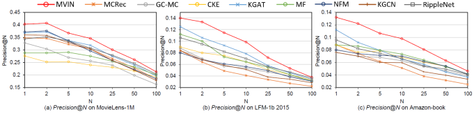
Table 2 and Figure 3 are the results of MVIN and the baselines, respectively (FM, NFM, CKF, GC-MC, MCRec, RippleNet, KGCN, KGAT), in click-through rate (CTR) prediction, i.e., taking a user-item pair as input and predicting the probability of the user engaging with the item. We adopt and , which are widely used in binary classification problems, to evaluate the performance of CTR prediction. For those of top- recommendation, selecting items with highest predicted click probability for each user and choose to evaluate the recommended sets. We have the following observations:
-
•
MVIN yields the best performance of all the datasets and achieves performance gains of 1.2% , 2.5%, and 2.2% on ML-1M, LFM-1b, and AZ-book, respectively. Also, MVIN achieves outstanding performance in top- recommendation, as shown in Figure 3.
-
•
The two path-based baselines RippleNet and KGAT outperform the two CF-based methods FM and NFM, indicating that KG is helpful for recommendation. Furthermore, although RippleNet and KGAT achieve excellent performance, they still do not outperform MVIN. This is because RippleNet neither incorporates user click history items into user representation nor does it introduces high-order connectivities, and KGAT does not mix GCN layer information and not v consider user preferences when collecting KG information.
-
•
For the other baselines KGCN and MCRec, their relatively bad performance is attributed to their not fully utilizing information from user click items. In contrast, MVIN would first enrich a user representation by user click items and all relevant entities in KG and then weighted the nearby entities and emphasize the most important ones. Also, KGCN only uses GCN in each layer, which does not allow contrast on neighborhood layers. Furthermore, MCRec requires finer defined meta paths, which requires manual labor and domain knowledge.
-
•
To our surprise, the CF-based NFM achieves good performance on LFM-1b and AZ-book, even outperforming the KG-aware baseline KGCN, and achieves results comparable to RippleNet. Upon investigation, we found that this is because we enriched its item representation by feeding the embeddings of its connected entities. In addition, NFM’s design involves modeling higher-order and non-linear feature interactions and thus better captures interactions between user and item embeddings. These observation conform to (Wang et al., 2019a).
-
•
The regularization-based CKE is outperformed by NFM. CKE does not make full use of the KG because it is only regularized by correct triplets from KG. Also, CKE neglects high-order connectivities.
-
•
Although GC-MC has introduced high-order connectivity into user and item representations, it achieves comparably weak performance as it only utilizes a user-item bipartite graph and ignores semantic information between KG entities.
5.4. Study of MVIN
| Ablation component | Components | ML-1M | LFM-1b | AZ-book | |||||
| UO(e) | UO(r) | UO(k) | ML(w) | ML(d) | SW | AUC | AUC | AUC | |
| N/A | ✔ | ✔ | ✔ | ✔ | ✔ | ✔ | .9318 | .9658 | .8739 |
| w/o UO(e) | ✔ | ✔ | ✔ | ✔ | ✔ | .9299 (-0.2%) | .9617 (-0.4%)* | .8672 (-0.8%)* | |
| w/o UO(r) | ✔ | ✔ | ✔ | ✔ | ✔ | .9305 (-0.1%) | .9638 (-0.2%) | .8705 (-0.4%)* | |
| w/o UO(k) | ✔ | ✔ | ✔ | ✔ | ✔ | .9247 (-0.7%)* | .9598 (-0.6%)* | .8573 (-1.8%)* | |
| w/o ML(w) | ✔ | ✔ | ✔ | ✔ | ✔ | .9289 (-0.3%)* | .9621 (-0.4%)* | .8683 (-0.6%)* | |
| w/o ML | ✔ | .9283(-0.4%)* | .9613 (-0.5%)* | .8637 (-1.2%)* | |||||
| w/o SW | ✔ | ✔ | ✔ | ✔ | ✔ | .9276 (-0.5%)* | .9567 (-0.9%)* | .8642 (-1.1%)* | |
We conducted an ablation study to verify the effectiveness of the proposed components. We also provide an in-depth exploration of the entity view.
5.4.1. User-Oriented Information
The ablation study results are shown in Table 3. After removing the proposed user-oriented relation attention UO(r) and user-oriented entity projection UO(e) modules, MVIN and MVIN perform worse than MVIN in all datasets. Thus considering user preferences when aggregating entities and relations in KG improves recommendation results.

5.4.2. KG-enhanced User-Oriented Information
To enhance user-oriented information, we enrich the user representation using KG information as a pre-processing step. Here, we denote MVIN without KG-enhanced user-oriented information as MVIN. We compare the performance of MVIN and MVIN. Table 3 shows that the former outperforms the latter by a large margin, which confirms that KG-enhanced user representation improves user-oriented information.
Moreover, we conducted a case study to understand the effect of KG-enhanced user-oriented information incorporated with user-entity interaction. Given the attention weights learned by MVIN in Figure 4(a), user puts only slightly more value on the author of Life After Life. However, Figure 4(b) shows that MVIN puts much more attention on the author when information on user-interacted items is provided. Furthermore, in Figure 4(b), we find user ’s interacted items— (One Good Turn), (Behind the Scenes at the Museum), and (Case Histories)—are all written by Kate Atkinson. This demonstrates that MVIN outperforms MVIN because it captures the most important view that user sees: item Life After Life, a book by Kate Atkinson.
5.4.3. Mixing layer-wise GCN information
In the mixing layer, the wide part ML(w) allows MVIN to represent general layer-wise neighborhood mixing. To study the effect of ML(w), we remove the wide part from MVIN, denoted as MVIN. Table 3 shows a drop in performance, suggesting that the mixing of features from different distances improves recommendation performance.

5.4.4. Mixing layer-wise GCN information (at high neighbor sampling size )
It has shown that in homogeneous graphs the benefit of the mixing layer depends on the homophily level.666The homophily level indicates the likelihood of a node forming a connection to a neighbor with the same label. In MVIN, the mixing layer works in KGs, i.e., heterogeneous graphs; we also investigate its effect (ML(w)) at different sampling sizes of neighborhood nodes . With a large , entities in KG connect to more different entities, which is similar to a low homophily level. Figure 5 shows that ML(w) is effective in heterogeneous graphs. In addition, increases the performance gap between MVIN and MVIN. We conclude that the mixing layer not only improves MVIN performance but is indispensable for large .
5.4.5. High-order connectivity information
In addition to the wide part in the mixing layer, the proposed deep part allows MVIN to aggregate high-order connectivity information. Figure 3 shows that after removing the mixing layer (ML), MVIN performs poorly compared to MVIN, demonstrating the significance of high-order connectivity. This observation is consistent with (Wang et al., 2019a; Wang et al., 2019c; Ying et al., 2018).
5.4.6. Stage-wise Training
Removing the stage-wise training (SW) shown by MVIN deteriorates performance, showing that stage-wise training helps MVIN achieve better performance by collecting more entity relations from the KG to approximate a panoramic view of the whole neighborhood. Note that compared to KGAT, the state-of-the-art baseline model which samples the whole neighbor entities in KG, MVIN refers to a limited number of entities in KG but still significantly outperforms all baselines (at -value = 0.01), which confirms again the effectiveness of the proposed MVIN.
| size () | 4 | 8 | 16 | 32 | 64 |
| ML-1M | .9210 | .9247 | .9255 | .9269 | .9276 |
| LFM-1b | .9299 | .9368 | .9433 | .9498 | .9567 |
| AZ-book | .8508 | .8613 | .8616 | .8642 | .8631 |
| size () | 4 | 8 | 16 | 32 | 64 |
| ML-1M | .9246 | .9254 | .9258 | .9264 | .9252 |
| LFM-1b | .9427 | .9430 | .9433 | .9429 | .9415 |
| AZ-book | .8590 | .8601 | .8594 | .8610 | .8593 |
| hops | 0 | 1 | 2 | 3 |
| ML-1M | .9257 | .9262 | .9233 | .9244 |
| LFM-1b | .9317 | .9438 | .9429 | .9415 |
| AZ-book | .8557 | .8576 | .8555 | .8572 |
| hops | 0 | 1 | 2 | 3 |
| ML-1M | n/a | .9261 | .9267 | .9262 |
| LFM-1b | n/a | .9438 | .9445 | .9447 |
| AZ-book | n/a | .8568 | .8611 | .8618 |
| hops | 0 | 1 | 2 | 3 |
| ML-1M | n/a | .9261 | .9269 | .9250 |
| LFM-1b | n/a | .9438 | .9441 | .9440 |
| AZ-book | n/a | .8552 | .8621 | .8613 |
| 4 | 8 | 16 | 32 | 64 | 128 | |
| ML-1M | .9037 | .9217 | .9259 | .9279 | .9250 | .9247 |
| LFM-1b | .9247 | .9468 | .9538 | .9574 | .9562 | .9538 |
| AZ-book | .8353 | .8471 | .8616 | .8664 | .8598 | .8539 |
5.5. Parameter Sensitivity
Below, we investigate the parameter sensitivity in MVIN.
Preference set sample size
Table 4 shows that the performance of MVIN improves when is set to a larger value, with the exception of AZ-book. MVIN achieves the best performance on AZ-book when is set to 32, which we attribute to its low number of user-interacted items, as shown in Table 1. That is, when there are few user-interacted items, a small still allows MVIN to find enough information to represent the user.
Neighborhood entity sample size
The influence of the size of neighborhood nodes is shown in Table 4. MVIN achieves the best performance when this is set to 16 or 32, perhaps due to the noise introduced when is too large.
Number of preference hops
The impact of is shown in Table 5. We conducted experiments with set to 0, that is, we only use user-clicked items to calculate user representation. The results show that when hop is set to 1, MVIN achieves the best performance, whereas again larger values of result in less relevant entities and thus more noise, consistent with (Wang et al., 2018b).
Number of wide hops and deep hops
Table 5 shows the effect of varying the number of the wide hops and deep hops . MVIN achieves better performance when the number of hops is set to 2 over 1, suggesting that increasing the hops enables the modeling of high-order connectivity and hence enhances the performance. However, the performance drops when the number of hops becomes even larger, i.e., 3, suggesting that considering second-order relations among entities is sufficient, consistent with (Sha et al., 2019; Wang et al., 2019d).
Dimension of embedding size
The results when varying the embedding size are shown in Table 6. Increasing initially boosts the performance as a larger contains more useful information of users and entities, whereas setting too large leads to overfitting.
6. Conclusion
We propose MVIN, a GNN-based recommendation model which improves representations of items from both the user view and the entity view. Given both user- and entity-view features, MVIN gathers personalized knowledge information in the KG (user view) and further considers the difference among layers (entity view) to ultimately enhance item representations. Extensive experiments show the superiority of MVIN. In addition, the ablation experiment verifies the effectiveness of each proposed component.
As the proposed components are general, the method could also be applied to leverage structural information such as social networks or item contexts in the form of knowledge graphs. We believe MVIN can be widely used in related applications.
References
- (1)
- Abu-El-Haija et al. (2019) Sami Abu-El-Haija, Bryan Perozzi, Amol Kapoor, Hrayr Harutyunyan, Nazanin Alipourfard, Kristina Lerman, Greg Ver Steeg, and Aram Galstyan. 2019. MixHop: Higher-Order Graph Convolutional Architectures via Sparsified Neighborhood Mixing. CoRR abs/1905.00067 (2019). arXiv:1905.00067 http://arxiv.org/abs/1905.00067
- An et al. (2019) Mingxiao An, Fangzhao Wu, Chuhan Wu, Kun Zhang, Zheng Liu, and Xing Xie. 2019. Neural News Recommendation with Long- and Short-term User Representations. https://doi.org/10.18653/v1/P19-1033
- Barshan and Fieguth (2015) Elnaz Barshan and Paul Fieguth. 2015. Stage-wise Training: An Improved Feature Learning Strategy for Deep Models. In Proceedings of the 1st International Workshop on Feature Extraction: Modern Questions and Challenges at NIPS 2015 (Proceedings of Machine Learning Research). PMLR, 49–59. http://proceedings.mlr.press/v44/Barshan2015.html
- Cao et al. (2019a) Yixin Cao, Xiang Wang, Xiangnan He, Zikun Hu, and Tat-Seng Chua. 2019a. Unifying Knowledge Graph Learning and Recommendation: Towards a Better Understanding of User Preferences. CoRR abs/1902.06236 (2019). arXiv:1902.06236 http://arxiv.org/abs/1902.06236
- Cao et al. (2019b) Yixin Cao, Xiang Wang, Xiangnan He, Zikun Hu, and Tat-Seng Chua. 2019b. Unifying Knowledge Graph Learning and Recommendation: Towards a Better Understanding of User Preferences. In The World Wide Web Conference (WWW ’19). Association for Computing Machinery, New York, NY, USA, 151–161. https://doi.org/10.1145/3308558.3313705
- Hamilton et al. (2017) William L. Hamilton, Rex Ying, and Jure Leskovec. 2017. Inductive Representation Learning on Large Graphs. In NIPS.
- He and Chua (2017) Xiangnan He and Tat-Seng Chua. 2017. Neural Factorization Machines for Sparse Predictive Analytics. In Proceedings of the 40th International ACM SIGIR Conference on Research and Development in Information Retrieval (Shinjuku, Tokyo, Japan) (SIGIR ’17). Association for Computing Machinery, New York, NY, USA, 355–364. https://doi.org/10.1145/3077136.3080777
- Hu et al. (2018a) Binbin Hu, Chuan Shi, Wayne Zhao, and Philip Yu. 2018a. Leveraging Meta-path based Context for Top- N Recommendation with A Neural Co-Attention Model. https://doi.org/10.1145/3219819.3219965
- Hu et al. (2018b) Binbin Hu, Chuan Shi, Wayne Xin Zhao, and Philip S. Yu. 2018b. Leveraging Meta-path Based Context for Top- N Recommendation with A Neural Co-Attention Model. In Proceedings of the 24th ACM SIGKDD International Conference on Knowledge Discovery (KDD ’18). https://doi.org/10.1145/3219819.3219965
- Huang et al. (2018) Jin Huang, Wayne Xin Zhao, Hongjian Dou, Ji-Rong Wen, and Edward Y. Chang. 2018. Improving Sequential Recommendation with Knowledge-Enhanced Memory Networks. In The 41st International ACM SIGIR Conference (SIGIR ’18). ACM, New York, NY, USA, 505–514. https://doi.org/10.1145/3209978.3210017
- Jamali and Ester (2010) Mohsen Jamali and Martin Ester. 2010. A Matrix Factorization Technique with Trust Propagation for Recommendation in Social Networks. In Proceedings of the Fourth ACM Conference on Recommender Systems (Barcelona, Spain) (RecSys ’10). ACM, New York, NY, USA, 135–142. https://doi.org/10.1145/1864708.1864736
- Kipf and Welling (2016) Thomas N. Kipf and Max Welling. 2016. Semi-Supervised Classification with Graph Convolutional Networks. arXiv e-prints, Article arXiv:1609.02907 (Sep 2016), arXiv:1609.02907 pages. arXiv:1609.02907 [cs.LG]
- Koncel-Kedziorski et al. (2019) Rik Koncel-Kedziorski, Dhanush Bekal, Yi Luan, Mirella Lapata, and Hannaneh Hajishirzi. 2019. Text Generation from Knowledge Graphs with Graph Transformers. In Proceedings of the 2019 Conference of the North American Chapter of the Association for Computational Linguistics. 2284–2293. https://doi.org/10.18653/v1/N19-1238
- Koren et al. (2009) Yehuda Koren, Robert Bell, and Chris Volinsky. 2009. Matrix factorization techniques for recommender systems. Computer 42, 8.
- Li et al. (2019) Wei Li, Jingjing Xu, Yancheng He, ShengLi Yan, Yunfang Wu, and Xu Sun. 2019. Coherent Comments Generation for Chinese Articles with a Graph-to-Sequence Model. In Proceedings of the 57th Annual Meeting of the Association for Computational Linguistics. Association for Computational Linguistics, Florence, Italy, 4843–4852. https://doi.org/10.18653/v1/P19-1479
- Mikolov et al. (2013) Tomas Mikolov, Ilya Sutskever, Kai Chen, Greg Corrado, and Jeffrey Dean. 2013. Distributed Representations of Words and Phrases and their Compositionality. CoRR abs/1310.4546 (2013). arXiv:1310.4546 http://arxiv.org/abs/1310.4546
- Oh et al. (2014) Kyo-Joong Oh, Won-Jo Lee, Chae-Gyun Lim, and Ho-Jin Choi. 2014. Personalized news recommendation using classified keywords to capture user preference. In Proceedings of 16th IEEE ICACT. 1283–1287.
- Rendle et al. (2011) Steffen Rendle, Zeno Gantner, Christoph Freudenthaler, and Lars Schmidt-Thieme. 2011. Fast Context-aware Recommendations with Factorization Machines. In Proceedings of the 34th International ACM SIGIR Conference (SIGIR ’11). ACM, New York, NY, USA, 635–644. https://doi.org/10.1145/2009916.2010002
- Schein et al. (2002) Andrew I Schein, Alexandrin Popescul, Lyle H Ungar, and David M Pennock. 2002. Methods and metrics for cold-start recommendations. In Proceedings of the 25th ACM SIGIR. 253–260.
- Sha et al. (2019) Xiao Sha, Zhu Sun, and Jie Zhang. 2019. Attentive Knowledge Graph Embedding for Personalized Recommendation. arXiv e-prints, Article arXiv:1910.08288 (Oct 2019), arXiv:1910.08288 pages. arXiv:1910.08288 [cs.IR]
- Sun et al. (2018) Zhu Sun, Jie Yang, Jie Zhang, Alessandro Bozzon, Long-Kai Huang, and Chi Xu. 2018. Recurrent Knowledge Graph Embedding for Effective Recommendation. In Proceedings of the 12th ACM Conference on Recommender Systems (Vancouver, British Columbia, Canada) (RecSys ’18). ACM, New York, NY, USA, 297–305. https://doi.org/10.1145/3240323.3240361
- Tai et al. (2019) Chang-You Tai, Meng-Ru Wu, Yun-Wei Chu, and Shao-Yu Chu. 2019. GraphSW: a training protocol based on stage-wise training for GNN-based Recommender Model. arXiv e-prints, Article arXiv:1908.05611, arXiv:1908.05611 pages. arXiv:1908.05611 [cs.IR]
- van den Berg et al. (2017) Rianne van den Berg, Thomas N Kipf, and Max Welling. 2017. Graph Convolutional Matrix Completion. arXiv preprint arXiv:1706.02263 (2017).
- Wang et al. (2018b) Hongwei Wang, Fuzheng Zhang, Jialin Wang, Miao Zhao, Wenjie Li, Xing Xie, and Minyi Guo. 2018b. Ripple Network: Propagating User Preferences on the Knowledge Graph for Recommender Systems. CoRR abs/1803.03467 (2018). arXiv:1803.03467 http://arxiv.org/abs/1803.03467
- Wang et al. (2018c) Hongwei Wang, Fuzheng Zhang, Xing Xie, and Minyi Guo. 2018c. DKN: Deep Knowledge-Aware Network for News Recommendation. In Proceedings of the 2018 World Wide Web Conference (Lyon, France) (WWW ’18). International World Wide Web Conferences Steering Committee, Republic and Canton of Geneva, Switzerland, 1835–1844. https://doi.org/10.1145/3178876.3186175
- Wang et al. (2018) Hongwei Wang, Fuzheng Zhang, Xing Xie, and Minyi Guo. 2018. DKN: Deep Knowledge-Aware Network for News Recommendation. arXiv e-prints, Article arXiv:1801.08284 (Jan 2018), arXiv:1801.08284 pages. arXiv:1801.08284 [stat.ML]
- Wang et al. (2019c) Hongwei Wang, Fuzheng Zhang, Mengdi Zhang, Jure Leskovec, Miao Zhao, Wenjie Li, and Zhongyuan Wang. 2019c. Knowledge Graph Convolutional Networks for Recommender Systems with Label Smoothness Regularization. CoRR abs/1905.04413 (2019). arXiv:1905.04413 http://arxiv.org/abs/1905.04413
- Wang et al. (2019d) Hongwei Wang, Miao Zhao, Xing Xie, Wenjie Li, and Minyi Guo. 2019d. Knowledge Graph Convolutional Networks for Recommender Systems. CoRR abs/1904.12575 (2019). arXiv:1904.12575 http://arxiv.org/abs/1904.12575
- Wang et al. (2017) Q. Wang, Z. Mao, B. Wang, and L. Guo. 2017. Knowledge Graph Embedding: A Survey of Approaches and Applications. IEEE Transactions on Knowledge and Data Engineering 29, 12 (Dec 2017), 2724–2743. https://doi.org/10.1109/TKDE.2017.2754499
- Wang et al. (2019a) Xiang Wang, Xiangnan He, Yixin Cao, Meng Liu, and Tat-Seng Chua. 2019a. KGAT: Knowledge Graph Attention Network for Recommendation. CoRR abs/1905.07854 (2019). arXiv:1905.07854 http://arxiv.org/abs/1905.07854
- Wang et al. (2019b) Xiang Wang, Xiangnan He, Meng Wang, Fuli Feng, and Tat-Seng Chua. 2019b. Neural Graph Collaborative Filtering. CoRR abs/1905.08108 (2019). arXiv:1905.08108 http://arxiv.org/abs/1905.08108
- Wang et al. (2018a) Xiang Wang, Dingxian Wang, Canran Xu, Xiangnan He, Yixin Cao, and Tat-Seng Chua. 2018a. Explainable Reasoning over Knowledge Graphs for Recommendation. CoRR abs/1811.04540 (2018). arXiv:1811.04540 http://arxiv.org/abs/1811.04540
- Wu et al. (2019) Chuhan Wu, Fangzhao Wu, Mingxiao An, Jianqiang Huang, Yongfeng Huang, and Xing Xie. 2019. NPA: Neural News Recommendation with Personalized Attention. arXiv e-prints, Article arXiv:1907.05559 (Jul 2019), arXiv:1907.05559 pages. arXiv:1907.05559 [cs.IR]
- Wu et al. (2019) Le Wu, Peijie Sun, Yanjie Fu, Richang Hong, Xiting Wang, and Meng Wang. 2019. A Neural Influence Diffusion Model for Social Recommendation. CoRR abs/1904.10322 (2019). arXiv:1904.10322 http://arxiv.org/abs/1904.10322
- Xin et al. (2019) Xin Xin, Xiangnan He, Yongfeng Zhang, Yongdong Zhang, and Joemon M. Jose. 2019. Relational Collaborative Filtering: Modeling Multiple Item Relations for Recommendation. CoRR abs/1904.12796 (2019). arXiv:1904.12796 http://arxiv.org/abs/1904.12796
- Ying et al. (2018) Rex Ying, Ruining He, Kaifeng Chen, Pong Eksombatchai, William L. Hamilton, and Jure Leskovec. 2018. Graph Convolutional Neural Networks for Web-Scale Recommender Systems. CoRR abs/1806.01973 (2018). arXiv:1806.01973 http://arxiv.org/abs/1806.01973
- Yu et al. (2014) Xiao Yu, Xiang Ren, Yizhou Sun, Quanquan Gu, Bradley Sturt, Urvashi Khandelwal, Brandon Norick, and Jiawei Han. 2014. Personalized Entity Recommendation: A Heterogeneous Information Network Approach. In Proceedings of the 7th ACM International Conference on Web Search and Data Mining (New York, New York, USA) (WSDM ’14). ACM, New York, NY, USA, 283–292. https://doi.org/10.1145/2556195.2556259
- Zhang et al. (2016a) Fuzheng Zhang, Nicholas Jing Yuan, Defu Lian, Xing Xie, and Wei-Ying Ma. 2016a. Collaborative Knowledge Base Embedding for Recommender Systems. In Proceedings of the 22Nd ACM SIGKDD International Conference on Knowledge Discovery and Data Mining (KDD ’16). 353–362. https://doi.org/10.1145/2939672.2939673
- Zhang et al. (2016b) Fuzheng Zhang, Nicholas Jing Yuan, Defu Lian, Xing Xie, and Wei-Ying Ma. 2016b. Collaborative Knowledge Base Embedding for Recommender Systems. In Proceedings of the 22Nd ACM SIGKDD International Conference on Knowledge Discovery and Data Mining (San Francisco, California, USA) (KDD ’16). ACM, New York, NY, USA, 353–362. https://doi.org/10.1145/2939672.2939673
- Zhang et al. (2018) Yongfeng Zhang, Qingyao Ai, Xu Chen, and Pengfei Wang. 2018. Learning over Knowledge-Base Embeddings for Recommendation. ArXiv abs/1803.06540 (2018).
- Zhao et al. (2017) Huan Zhao, Quanming Yao, Jianda Li, Yangqiu Song, and Dik Lun Lee. 2017. Meta-Graph Based Recommendation Fusion over Heterogeneous Information Networks. In Proceedings of the 23rd ACM SIGKDD International Conference on Knowledge Discovery and Data Mining (Halifax, NS, Canada) (KDD ’17). ACM, New York, NY, USA, 635–644. https://doi.org/10.1145/3097983.3098063
- Zhao et al. (2018) Wayne Xin Zhao, Gaole He, Hong-Jian Dou, Jin Huang, Siqi Ouyang, and Ji-Rong Wen. 2018. KB4Rec: A Dataset for Linking Knowledge Bases with Recommender Systems. CoRR abs/1807.11141 (2018). arXiv:1807.11141 http://arxiv.org/abs/1807.11141
- Zheng et al. (2017) Lei Zheng, Vahid Noroozi, and Philip S. Yu. 2017. Joint Deep Modeling of Users and Items Using Reviews for Recommendation. CoRR abs/1701.04783 (2017). arXiv:1701.04783 http://arxiv.org/abs/1701.04783