Multiwavelength Analysis of a Nearby Heavily Obscured AGN in NGC 449
Abstract
We presented the multiwavelength analysis of a heavily obscured active galactic nucleus (AGN) in NGC 449. We first constructed a broadband X-ray spectrum using the latest NuSTAR and XMM-Newton data. Its column density () and photon index () were reliably obtained by analyzing the broadband X-ray spectrum. However, the scattering fraction and the intrinsic X-ray luminosity could not be well constrained. Combined with the information obtained from the mid-infrared (mid-IR) spectrum and spectral energy distribution (SED) fitting, we derived its intrinsic X-ray luminosity () and scattering fraction (). In addition, we also derived the following results: (1). The mass accretion rate of central AGN is about , and the Eddington ratio is ; (2). The torus of this AGN has a high gas-to-dust ratio (); (3). The host galaxy and the central AGN are both in the early stage of co-evolution.
1 Introduction
It is well known that active galactic nuclei (AGNs) are powered by the accretion of surrounding matter by supermassive black holes (SMBHs). The emission of AGNs covers almost the whole electromagnetic band. The AGNs’ radiations at different wavelengths arise from their diverse structures. For example, the significant emission of the accretion disk is in the ultraviolet (UV) to the optical band (e.g., Richstone & Schmidt, 1980), while the emission of the torus is in the mid-infrared (mid-IR) band (e.g., Antonucci, 1993). The diverse information can be derived from the emission of AGNs at different wavelengths. To fully understand an AGN, it is often necessary to study with the multi-bands.
The classification of AGNs usually utilizes the observation features of different wavelengths. For instance, based on the characteristics of the optical emission lines, AGNs can be classified into type 1 and type 2 (e.g., Khachikian & Weedman, 1974). The AGN unified model proposes that different AGN types are caused by different viewing angles with an obscuring torus (e.g., Antonucci, 1993; Urry & Padovani, 1995; Netzer, 2015). Since the X-ray emission has a strong pierce, the X-ray emission of AGNs is usually subject to little absorption. Based on the column density () of the X-ray absorption, AGNs can be classified into four categories: unobscured (), obscured (), heavily obscured (), and Compton-thick (, e.g., Comastri, 2004). Many studies have also regarded the source with a column density of as Compton-thick AGN (CT-AGN, e.g., Risaliti et al., 1999; Kammoun et al., 2019).
Some studies have pointed out that most AGNs were heavily obscured (e.g., Hickox & Alexander, 2018). The heavily obscured AGNs are believed to be in an early phase of the evolutionary scenario of AGNs, which is a rapid growth state of central SMBH (e.g., Goulding et al., 2011). The host galaxies of heavily obscured AGNs are also in an early phase of the evolutionary scenario of galaxies. For instance, Kocevski et al. (2015) pointed out that heavily obscured AGNs were twice as likely to be hosted by late-type galaxies relative to unobscured AGNs. As a class of the most luminous and persistent X-ray sources in the universe, AGNs contribute the vast majority of Cosmic X-ray Background (CXB, e.g., Ueda et al., 2014) in the 1 to 200 – 300 keV. The heavily obscured AGNs and CT-AGNs are significant contributors to the hump of the CXB emission at 30 keV (e.g., Marshall et al., 1980; Ajello et al., 2008).
The single-band analysis for AGNs can only derive a part of their properties. For example, we can derive the column density in the line-of-sight (LOS) direction by fitting X-ray spectra. Using the spectral energy distributions (SEDs) from the UV to the far-IR, we can derive the star formation rates (SFRs) of the host galaxies, stellar masses of the host galaxies, and AGN luminosities. To fully understand heavily obscured AGNs, their host galaxies, and their co-evolution, we first derive their properties through multi-band analysis.
The heavily obscured AGNs usually present a complex spectral shape in their X-ray waveband. Theoretically, the soft X-ray emission (E 2 keV) of heavily obscured AGNs will be heavily (entirely) absorbed. Even in many CT AGNs, the soft X-ray is not entirely absorbed, because the emission from the AGNs’ scattered and the host galaxy can be observed (e.g., Turner et al., 1997; LaMassa et al., 2012). As the energy increases, the absorption of X-ray emission (E10 keV) is gradually reduced or cut-off. The hard X-ray of heavily obscured AGN is dominated by the reflected component, the so-called Compton reflection continuum characterized by a broad bump peaking around 20–30 keV (e.g. Comastri, 2004). One of the most prominent features in the X-ray spectrum of heavily obscured AGN is the neutral iron K emission line at 6.4 keV. However, the X-ray spectra of some heavily obscured AGNs show a weak (or absent) iron K emission line (Boorman et al., 2018), especially the heavily obscured AGNs beyond the local universe. To accurately determine the column density of the gas and recover the intrinsic X-ray flux of AGNs, we require proper modeling of the physical processes in the AGNs that self-consistently account for the transmitted emission, Compton-scattered reflected component and the fluorescent line flux. Such modeling may also constrain the geometry of the torus and view angle. Over the past several years, a series of X-ray spectral models (e.g., Murphy & Yaqoob, 2009; Baloković et al., 2018) are created with assumed different geometries (spherical, toroidal, or clumpy). Many recent studies use these models to constrain the parameters of AGNs (Gandhi et al., 2017; Kammoun et al., 2019; LaMassa et al., 2019; Toba et al., 2020).
From the UV to the optical band, the continua of the heavily obscured AGNs are masked by the emission of the host galaxies, so we can only observe their high-ionized emission lines and obtain little information about them. It is difficult to constrain the gas column density along LOS for the AGNs with low-quality X-ray spectra. However, we can estimate the gas column density using the luminosity ratio of X-ray to high-ionized emission lines (e.g., Maiolino et al., 1998; Cappi et al., 2006; Gilli et al., 2010; Lanzuisi et al., 2015). The mid-IR emission of the AGNs is usually less suppressed due to the low optical depth. The contribution of AGNs can be easily decomposed in the mid-IR spectra. In addition, for heavily obscured AGNs, we can also observe a strong silicon absorption line at 9.7 µm. The dust in the torus can be derived using silicon absorption strength (e.g., Xu et al., 2020). By the SED fitting, we can accurately obtain the contribution of the AGNs, the AGN luminosities, and some parameters about their host galaxies. So the multi-band data can provide us with more comprehensive information on heavily obscured AGNs.
NGC 449 (also known as Mrk 1) is a nearby (z=0.01595, D67 Mpc) Seyfert 2 galaxy, and its center hosts a heavily obscured AGN. It was observed by the XMM-Newton X-ray telescope (Jansen et al., 2001) in 2004. Guainazzi et al. (2005) fitted the X-ray spectrum and constrained the column density () of this AGN. Moreover, some studies also derived its column density by using the ratio of X-ray to high-ionized emission lines ([O III]5007, [Ne V]3426) luminosity (Heckman et al., 2005; Gilli et al., 2010). These results indicated that the X-ray is severely absorbed and that even the AGN may be a CT-AGN. However, these results did not constrain its column density well. To better constrain its column density and other properties, the spectrum above 10 keV is necessary. Fortunately, this source was observed by the Nuclear Spectroscopic Telescope Array (NuSTAR, Harrison et al., 2013) in 2017. The NuSTAR data has still not been analyzed (or presented in previous work). Moreover, there are abundant data about NGC 449 in the archives, which can also help us to obtain more properties. So the motivation of our work is to constrain the properties of this heavily obscured AGN by multiwavelength analysis.
The structure of the paper is as follows. Section 2 describes the multiwavelength data and processing for NGC 449. In Section 3, we analyzed the multiwavelength data of this source in detail. Then, we discuss the implications of our results in Section 4. Finally, we present a summary of this work in Section 5. We adopt a concordance flat -cosmology with , , and (Planck Collaboration et al., 2020).
2 Multiwavelength data
2.1 X-Ray Observations and Data Reduction
A log of the XMM-Newton and NuSTAR observations analyzed herein is presented in Table 1, and the individual data sets are described in this section.
| ObsID | Observation date | Mission | Instrument(s) | Net Exposure | Net Counts |
|---|---|---|---|---|---|
| [ks] | |||||
| MOS1 | 11.4 | 249.90 | |||
| 0200430301 | 2004-01-09 | Newton | MOS2 | 11.5 | 222.31 |
| PN | 8.6 | 735.63 | |||
| 60360002002 | 2017-12-23 | NuSTAR | FPMA | 32.7 | 130.66 |
| FPMB | 32.6 | 126.67 |
2.1.1 XMM-Newton Observations
NGC 449 was observed by the XMM-Newton X-ray telescope (Jansen et al., 2001) for about 11.9 ks of exposure on January 9, 2004 (PI: Matteo Guainazzi, ObsID: 0200430301). The data is reduced in a standard manner using the XMM-Newton Science Analysis System (SAS, Gabriel et al., 2004) v17.0.0 and Current Calibration Files (CCF) of June 22, 2018. The spectra are extracted from a circular region (30 arcsec radius for PN and 25 arcsec radius for MOS) around the source, and the background spectra are taken from a nearby source-free circular region (80 arcsec radius for PN and 100 arcsec radius for MOS). The spectra are binned to have minimum counts of 10 per energy bin.
2.1.2 NuSTAR Observations
NGC 449 was also observed by the NuSTAR (Harrison et al., 2013) for about 32.7 ks of exposure on December 8, 2017 (ObsID: 60360002002). The data is processed using the NuSTAR data analysis software nustardas v1.9.5 available in heasoft v6.27.2 and CALDB released on August 13, 2020. The nupipeline script is used to produce calibrated and clean event files. We extract source spectra using the nuproducts task. The spectra are extracted from a 45 arcsec radius aperture centered on the source, while the background is extracted from a circular region with a 100 arcsec radius from a source-free region on the detector. To improve the spectral quality of NuSTAR, we try to combine the two spectra of FPMA and FPMB. The combined spectrum is also binned to have minimum counts of 10 per energy bin.
2.2 Mid-IR spectral Observations and Data Reduction
We search the archives for its mid-IR data. There is good mid-IR spectral data, covering wavelengths from 5 to 37 µm, observed by Spitzer’s IrsStare on February 5, 2009 (PI: Levenson, Nancy, ObsID: 25408000). The mid-IR spectrum was processed using the Spitzer data analysis software irs_merge v2.1 with the pipeline script (version: S18.18.0) on December 18, 2011. For more detailed processing of the mid-IR spectrum of this source, please refer to Section 2 of Lebouteiller et al. (2011).
2.3 Multiwavelength photometric data
To construct the SED for NGC 449, we search for available multi-band photometric data from different surveys or the archives of telescopes, i.e., the Sloan Digital Sky Survey (SDSS) Data Release 7 (Abazajian et al., 2009), the Two Micron All-Sky Survey (2MASS, Skrutskie et al., 2006), the Wide-field Infrared Survey Explorer (WISE, Wright et al., 2010), the AKARI and the Infrared Astronomical Satellite (IRAS). In total, we collect the photometric data for 17 filters. Among them, only the filter SDSS-u is in the UV band. There are three filters of the optical band, including SDSS-g, SDSS-r, and SDSS-i. The other filters are in the IR band, including four near-IR filters (SDSS-z, 2MASS-J, 2MASS-H, 2MASS-K), seven mid-IR filters (W1, W2, W3, W4, IRAS-PSC 25, AKARI-PSC 09, AKARI-PSC 18) and two far-IR filters (IRAS-PSC 60, IRAS-PSC 100). The details for photometric data and filters are listed in Table 2.
| Band | Wavelength | Flux | References |
|---|---|---|---|
| [µm] | [mJy] | ||
| SDSS-u | 0.3547 | (a) | |
| SDSS-g | 0.4767 | ||
| SDSS-r | 0.6226 | ||
| SDSS-i | 0.7615 | ||
| SDSS-z | 0.9123 | ||
| 2MASS-J | 1.234 | (b) | |
| 2MASS-H | 1.661 | ||
| 2MASS-K | 2.157 | ||
| WISE-W1 | 3.4 | (c) | |
| WISE-W2 | 4.6 | ||
| WISE-W3 | 12 | ||
| WISE-W4 | 22 | ||
| IRAS-PSC 25 | 25 | (d) | |
| IRAS-PSC 60 | 60 | ||
| IRAS-PSC 100 | 100 | ||
| AKARI-PSC 09 | 9 | (e) | |
| AKARI-PSC 18 | 18 |
3 Analysis of Multiwavelength data
3.1 X-Ray Spectral Analysis
In this section, we analyze the X-ray spectra of NGC 449 in Xspec v.12.11.0 (Arnaud, 1996). First, we use phenomenological modeling to determine whether there is variation in the spectra for the same energy range of XMM-Newton and NuSTAR. We then analyzed which components contributed to the X-ray spectra of this source. Based on the analysis of the X-ray components, we finally use the self-consistent and physical models to fit the X-ray spectra. All errors represent the 68.0% confidence intervals unless otherwise stated.
3.1.1 Testing for Variability Among Observations
To test whether there is significant variation in the spectra of two observations within the same energy range (3–10 keV), we need to compare their spectral shapes and fluxes. We can obtain them by fitting the X-ray spectra of this source. However, the data for this source is poor. To obtain more reliable properties, we use a phenomenological model to fit the spectra of XMM-Newton111The spectra of MOS1, MOS2 and PN are simultaneously fitted. and NuSTAR within the same energy range. The phenomenological model is written (in the Xspec terminology) as follows:
where accounts for the Galactic absorption which is fixed at a column density of .
| Mission | log() | /dof | |
|---|---|---|---|
| [] | |||
| Newton | 5.02/5 | ||
| NuSTAR | 31/17 |
Table 3 lists some properties of these two spectra within the same energy range. Their fluxes are the same within the error range. The spectral shape of XMM-Newton’s spectrum within the same energy range indicates that the X-ray emission of NGC 449 is seriously absorbed. Similarly, the NuSTAR observation of this source also presents a flat spectrum. The data in the same energy range are so poor that their photon indices cannot be well constrained. In short, these two observations have similar fluxes within the same energy range. Therefore, there is no significant variation in the X-ray emission for NGC 449 among these two observations.
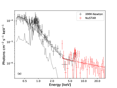
For subsequent X-ray spectrum analysis, we constitute a broadband X-ray spectrum using the X-ray spectra obtained with XMM-Newton and NuSTAR, which covers the 0.35–30 keV band (PN for XMM-Newton : 0.35–10.0 keV, NuSTAR : 3.0–30.0 keV).
3.1.2 Analysis of the basic components
In this section, our goal is to analyze which components contribute to the X-ray spectra of this source, providing support for subsequent model selection.
First, We use a powerlaw model () with a photon index of 2.17 to fit the broadband spectrum. Of course, the goodness of fit is poor (see the panel b of Figure 1). There is significant excess in the spectrum above 10 keV, which is a flat spectrum. So the broadband spectrum is again fitted by a broken powerlaw model (). Figure 1(c) shows the residuals of the broken powerlaw model. The best-fitting break energy is 3.93 keV. The low energy band is a steep spectrum (), and the high energy band is a flat spectrum (). Although its goodness of fit is significantly improved, there is still excess near 6.5 keV and 1 keV. Therefore, we also need to add two more models. Among them, a Gaussian model is used to fit the iron emission line near 6.5 keV, and the equivalent width (EW) of the iron emission line is 1.49 keV which is consistent with previous work (EW2 keV, Guainazzi et al., 2005). The other model (diffuse thermal emission) is used to match the excess near 1.0 keV. Finally, we obtain the best-fitting of the spectrum, as shown in Figure 1(a). The fitted parameters are listed in Table 4.
| Parameter | Power-law | Broken power-law | Broken+Gauss+Diffuse | |
|---|---|---|---|---|
| … | … | |||
| … | ||||
| (keV) | … | |||
| … | ||||
| lineE(keV) | … | … | ||
| (keV) | … | … | ||
| EW(keV) | … | … | 1.49 | |
| kT(keV) | … | … | ||
| /dof | 224.61/110 | 150.52/108 | 100.52/103 |
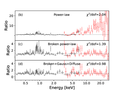
We find a flat spectrum above 3.71 keV by fitting the broadband spectrum, indicating that the emission of this source is seriously absorbed. Therefore, the reprocessed emission is dominant in hard X-rays. Theoretically, there should be a flat spectrum at energies below 3.71 keV. In fact, there is a steep spectrum below 3.71 keV with a photon index of 2.38. The power-law emission below 3.71 keV is most likely contributed by the scattered component of primary X-ray emission. Besides, the diffuse thermal emission and the iron emission line are required.
3.1.3 Pexmon model
According to the analysis in Section 3.1.2, we fit the spectrum using the neutral reflection model Pexmon (Nandra et al., 2007). The detailed model can be written as follows:
In this model, the component stands for the Galactic absorption is fixed at a column density of , represents the primary X-ray emission of the AGN, which is absorbed by obscured material (). The primary X-ray emission is scattered by ionized gas in the polar regions, while the scattering component is usually little or not absorbed. The soft scattering component into our LOS is represented by . Thus the parameters of are tied to the parameters of . The diffuse thermal radiation is denoted by , similar to Section 3.1.2. We use to represent the reprocessed emission.
The Pexmon model assumes a slab obscurer/reflector with an infinite optical depth, as may be expected in a standard geometrically thin accretion disc. The incident source in X-rays is the primary emission () from a hot electron corona. Therefore, the photon index and normalization of are tied to the identical parameters of . The cutoff energy of is fixed as 500 keV. We are not able to constrain the Fe abundance (tied to the elemental abundance), so we fix it to its best-fit value. The reflection fraction was fixed to -1 in the Pexmon fit.
This model fits the data well (/dof=101.38/105). The best-fitting and residuals are shown in Figure 2.

The Pexmon model implies that the X-ray emission of central AGN is absorbed by Compton-thick material with . The intrinsic 2–10 keV luminosity is . The photon index is 2.44, suggesting that the spectrum of central AGN is very soft. We note that the scattering component is found to be of the primary emission, and that the 2–10 keV luminosity of scattering component is . The diffuse thermal gas model () adequately describes the soft X-rays with a temperature kT = 0.82 keV. More best-fit parameters for the model are listed in Table 5.
| Parameter | Pexmon | Borus |
|---|---|---|
| kT(keV) | ||
| … | 25.0 | |
| 84.4 | ||
| /dof | 101.38/105 | 101.35/105 |
Note. — : the column density of LOS. : the average column density of torus. : the photon index of the X-ray spectrum. : the fraction of the scattering component. : the flux density of the scattering component. : the luminosity of the scattering component. kT: the temperature of diffuse thermal gas. : the half-opening angle of torus. : the inclination angle. : the absorbed flux density. : the absorbed luminosity. : the intrinsic flux density. : the intrinsic luminosity.
3.1.4 Borus model
Similarly, according to the analysis in Section 3.1.2, we refit the spectrum of the reprocessed emission using the Borus model (Baloković et al., 2018). Borus model is defined with the following command sequence in Xspec:
The , , and components are equivalent to the ones in the Pexmon fit. The represents LOS absorption at the redshift of the X-ray source (generally independent from the average column density of the torus), including Compton scattering losses out of the line of sight. The photon index and normalization of are also tied to the , and the cutoff energy is fixed as 500 keV. Some parameters can not be constrained, so we fix them to their best-fit values, i.e., half-opening angle, inclination angle, and iron abundance.
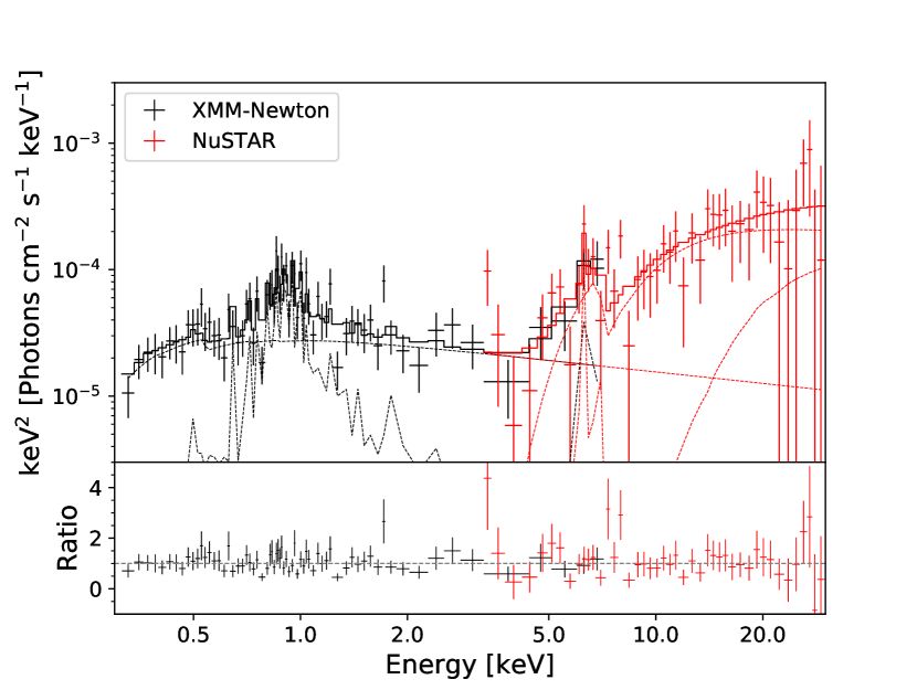
This model fits the data well (/dof=101.35/105). The best-fitting and residuals are shown in Figure 3. The column density of LOS is , and the average column density of the torus is about . The intrinsic 2–10 keV luminosity is . More best-fit parameters for the model are listed in Table 5.
Through the above analysis and the broadband X-ray spectrum fitting of two physical models (Pexmon and Borus), we have obtained some parameters about the AGN in NGC 449. Most of the parameters obtained by the two models are the identical within the error range, i.e., column density of LOS, the photon index, the luminosity of scattering component, the temperature of diffuse thermal gas, and the absorbed luminosity. These suggest that these parameters can be well constrained in the X-ray band. However, the fraction of the scattering component and the intrinsic luminosity can not be well constrained. Therefore, we need information from other bands to constrain these parameters.
3.2 Mid-IR spectrum Analysis
In this section, we use DeblendIRS222For more details, refer to http://www.denebola.org/ahc/deblendIRS/ (Hernán-Caballero et al., 2015) to analyze the mid-IR spectrum of NGC 449. DeblendIRS is an IDL package that fits the mid-IR spectra with a linear combination of three spectral templates, i.e., a “pure” AGN template, a “pure” stellar template, and a “pure” Polycyclic Aromatic Hydrocarbon (PAH, which accounts for the interstellar emission) template. The mid-IR spectra of the sources can be well decomposed into the contributions of different components using this package. Thus we obtain some physical properties of the AGNs and their host galaxies, such as the silicate strength333The silicate strength is defined as where and stand for the maximum flux density of the silicate line profile near 9.7 µm and the corresponding flux density of the underlying continuum profile,respectively. is a negative value, which means that the central radiation of the AGN is absorbed by the torus.The optical depth of the silicate absorption . (), spectral index (), AGN emission at rest-frame 6 µm, and 12 µm.
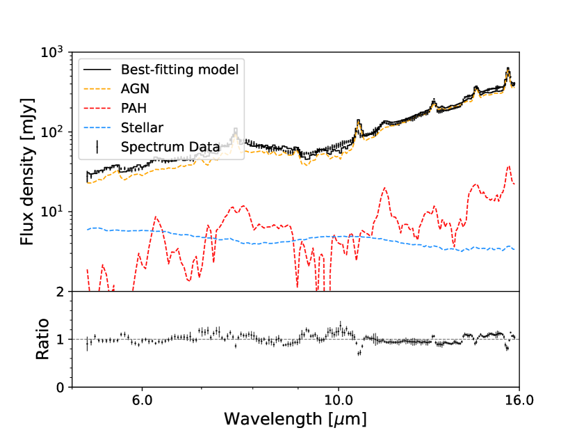
We use this package to fit the mid-IR spectrum (5 – 16 µm) and provide the best-fitting results. Figure 4 shows the best-fitting of the mid-IR spectrum of NGC 449. From this fitting, we derive a silicate strength of , a luminosity at 6 µm of , and a luminosity at 12 µm of .
3.3 Analysis of Multi-band SED
In this section, we analyze the Multi-band SED of this source using Code Investigating GALaxy Emission (CIGALE 2020.0, Boquien et al., 2019). CIGALE 2020.0 is an open python code designed to estimate the physical properties (i.e., SFR, stellar mass, AGN luminosity) of galaxies and AGNs. We fit the SED of NGC 449 with the same modules and parameters as Guo et al. (2020). For details, please refer to Section 3 of Guo et al. (2020).
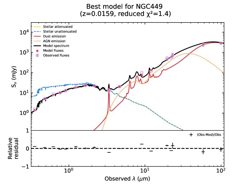
Figure 5 presents the best-fit SED for this source. In addition, we also obtain some physical parameters of NGC 449 by the SED fitting, such as SFR, stellar mass, and AGN luminosity. Table 6 lists several parameters that may be used in this work. The SFR estimate by the SED fitting is more dependent on the star formation history model, so we also use the calibration from Bell et al. (2005) to estimate SFR by the UV and IR luminosities, scaled to Chabrier (2003) initial mass function:
| (1) |
where is an estimation of the integrated 1216 – 3000Å rest-frame UV luminosity, and is the 8 – 1000 µm rest-frame IR luminosity. Both and (listed in Table 6) are in units of L⊙. The SFR of NGC 449 is 3.12 M⊙/yr which is estimated by the UV and IR luminosities.
| Parameter | Value |
|---|---|
| M∗ (M⊙) | |
| SFRSED (M⊙ yr-1) | |
| AGN Luminosity () | |
| /dof | 1.40 |
| ( L⊙) | |
| ( L⊙) | |
| SFRUV+IR (M⊙ yr-1) | 3.12 |
4 Results and Discussion
We have obtained some properties of NGC 449 through individual band analyses. However, some properties are not well-constrained. Combined with the multiband results, the properties of this source will be better constrained. In addition, we will also derive some other properties of this source.
4.1 The properties of the AGN central engine
The AGN at the center of NGC 449 is an optical type-2 AGN, so we cannot directly observe its central emission (e.g., accretion disk, corona). It is difficultly to understand the coronal (intrinsic) emission only by the X-ray spectrum fitting. For heavily obscured AGNs, the estimation of intrinsic luminosities (flux densities) is very dependent on the X-ray model employed. Although Table 5 presents the intrinsic 2–10 keV luminosities (flux densities) obtained by the Pexmon and Borus models, they are unreliable. To derive a reliable intrinsic luminosity, we had better estimate it in other ways. Fortunately, there is a very close correlation between 2–10 keV and mid-IR 12 µm luminosities of AGNs (e.g., Asmus et al., 2015). In Section 3.2, we have obtained the mid-IR 12 µm luminosity () of central AGN. We use Equation 2 of Asmus et al. (2015) to estimate intrinsic 2–10 keV luminosity of . Moreover, the fraction of the scattering component is also not well constrained. However, the Pexmon and Borus models have well-constrained the scattering luminosity, whose average value is . The relationship between the intrinsic luminosity and scattering luminosity is . So the scattering fraction of the X-ray emission of central AGN is about .
Since the UV-to-optical continuum of this source is mainly contributed by the host galaxy, we cannot obtain the bolometric emission of the accretion disk by SED fitting. However, the coronal and torus emissions can well track the thermal radiation of the accretion disk. So they can be used to estimate the bolometric luminosity of type-2 AGNs. Using the intrinsic 2–10 keV luminosity, we solve the Equation 21 of Marconi et al. (2004) to estimate the bolometric luminosity (bolometric correction ). This bolometric luminosity is consistent with that provided by Woo & Urry (2002).
The mass accretion rate is a measurement of SMBH mass growth and is related to bolometric luminosity. The relationship is written as , where is the efficiency that converts the rest-mass energy of accreted material into radiation. Assuming (Frank et al., 2002), we estimate the mass accretion rate of NGC449, which is . The Eddington ratio is a measurement of the SMBH accretion efficiency and is defined as , where is the bolometric luminosity of the AGN, is the Eddington luminosity of the AGN (). Using the SMBH mass () given in Woo & Urry (2002), we estimate the Eddington Luminosity to be . The Eddington ratio is about . The Eddington ratio of most CT-AGNs in the local universe is similar to our result (e.g., Tanimoto et al., 2022).
4.2 The properties of the torus
Previous studies have attempted to constrain the column density of NGC449 using XMM-Newton data or the ratio of X-ray to high-ionized emission lines ([O III]5007, [Ne V]3426) luminosities (Guainazzi et al., 2005; Heckman et al., 2005; Gilli et al., 2010). Those results suggested that the center of NGC449 hosted a CT-AGN. We use the latest X-ray data above 10 keV to construct a broadband X-ray spectrum. Compared with the previous studies, we can better constrain the parameters of the torus in Section 3.1. In the Pexmon model, the column density of the torus is obtained as , indicating that it may be a CT-AGN. In Section 3.1.4, we re-fit the broadband X-ray spectrum using the Borus model and obtain a series of parameters about torus. Among these parameters, the column density of LOS is , and the average column density of the torus is about , which is close to Compton-thick. In conclusion, the column density of this source we obtain is similar to that estimated by previous works (Guainazzi et al., 2005; Heckman et al., 2005; Gilli et al., 2010), but it is well-constrained.
In Section 3.2, we decomposed the contribution of AGN by the mid-IR spectrum fitting, and derived the silicate strength of the AGN component. Using the silicate strength, we can derive the optical depth of silicate absorption as . The optical depth of silicate absorption is a good way to track the dust in the torus, i.e., the V-band extinction is (Roche & Aitken, 1985). Therefore, the gas-to-dust ratio of the torus is ( is the average column density of torus). This gas-to-dust ratio is about 45 times that of the Galaxy (, Draine, 2003). Even this gas-to-dust ratio is higher than that of nearby CT-AGN in the Circinus galaxy (Tanimoto et al., 2019), which is the most obscured AGN in the nearby universe. Such a high gas-to-dust ratio of this source means that the radiation of the central AGN may have destroyed dust in the torus.
4.3 The evolutionary stage of the source
Many studies have suggested a co-evolution scheme between host galaxies and AGNs (e.g., Kormendy & Ho, 2013), such as relation (e.g., Ferrarese & Merritt, 2000), AGN feedback (e.g., Bower et al., 2006). Some studies have suggested that the host galaxies of heavily obscured AGNs appear to be at the stage of intense star formation (e.g., Hopkins et al., 2006). These intense star-forming activities may be associated with AGNs, i.e. AGNs trigger star formation of host galaxies.
NGC 449 is a late-type galaxy, meaning it is in an early stage of galaxy evolution. Its center hosts a heavily obscured AGN, which is considered to be at the early stage of AGN evolution. These suggest that the host galaxy and central AGN of NGC 449 are at the early stage of co-evolution. In Section 3.3, we derive some parameters about the host galaxy, including SFR and stellar mass. The specific star formation rate () of this source is approximately . This value is consistent with other star formation galaxies at similar redshifts (Salim et al., 2007). This result suggests that the central AGN does not appear to trigger intense star formation in its host galaxy.
5 Summary
We studied a heavily obscured AGN in NGC 449 using the multiwavelength data, which included NuSTAR, XMM-Newton, Spitzer, and multi-band photometric data. After, we analyzed its X-ray spectrum and obtained the column density (), the photon index (), the luminosity (flux density) of the scattering component, and the temperature () of diffuse thermal gas. However, some parameters could not be well constrained, i.e., the fraction of the scattering component, the intrinsic flux density, and luminosity. We fitted its mid-IR spectrum and decomposed the AGN contribution to derive some AGN parameters, and used its SED to obtain some parameters. Combining the information from the mid-IR spectrum and SED, we first derived the intrinsic X-ray luminosity () and the scattering fraction of primary X-ray emission (). In addition, we also derived the following results:
-
1.
The bolometric luminosity of the AGN is about . The mass accretion rate of central AGN is about , and the Eddington ratio is .
-
2.
The torus of this AGN has a high gas-to-dust ratio (), which is about 45 times that of the Galaxy. Such a high gas-to-dust ratio means that the radiation of the central AGN may have destroyed dust in the torus.
-
3.
The host galaxy and the central AGN are both in the early stage of co-evolution.
References
- Abazajian et al. (2009) Abazajian, K. N., Adelman-McCarthy, J. K., Agüeros, M. A., et al. 2009, ApJS, 182, 543, doi: 10.1088/0067-0049/182/2/543
- Ajello et al. (2008) Ajello, M., Greiner, J., Sato, G., et al. 2008, ApJ, 689, 666, doi: 10.1086/592595
- Antonucci (1993) Antonucci, R. 1993, ARA&A, 31, 473, doi: 10.1146/annurev.aa.31.090193.002353
- Arnaud (1996) Arnaud, K. A. 1996, in Astronomical Society of the Pacific Conference Series, Vol. 101, Astronomical Data Analysis Software and Systems V, ed. G. H. Jacoby & J. Barnes, 17
- Asmus et al. (2015) Asmus, D., Gandhi, P., Hönig, S. F., Smette, A., & Duschl, W. J. 2015, MNRAS, 454, 766, doi: 10.1093/mnras/stv1950
- Astropy Collaboration et al. (2013) Astropy Collaboration, Robitaille, T. P., Tollerud, E. J., et al. 2013, A&A, 558, A33, doi: 10.1051/0004-6361/201322068
- Baloković et al. (2018) Baloković, M., Brightman, M., Harrison, F. A., et al. 2018, ApJ, 854, 42, doi: 10.3847/1538-4357/aaa7eb
- Bell et al. (2005) Bell, E. F., Papovich, C., Wolf, C., et al. 2005, ApJ, 625, 23, doi: 10.1086/429552
- Boorman et al. (2018) Boorman, P. G., Gandhi, P., Baloković, M., et al. 2018, MNRAS, 477, 3775, doi: 10.1093/mnras/sty861
- Boquien et al. (2019) Boquien, M., Burgarella, D., Roehlly, Y., et al. 2019, A&A, 622, A103, doi: 10.1051/0004-6361/201834156
- Bower et al. (2006) Bower, R. G., Benson, A. J., Malbon, R., et al. 2006, MNRAS, 370, 645, doi: 10.1111/j.1365-2966.2006.10519.x
- Cappi et al. (2006) Cappi, M., Panessa, F., Bassani, L., et al. 2006, A&A, 446, 459, doi: 10.1051/0004-6361:20053893
- Chabrier (2003) Chabrier, G. 2003, PASP, 115, 763, doi: 10.1086/376392
- Comastri (2004) Comastri, A. 2004, Compton Thick AGN: the dark side of the X-ray background (Springer Netherlands), 245–272
- Draine (2003) Draine, B. T. 2003, ARA&A, 41, 241, doi: 10.1146/annurev.astro.41.011802.094840
- Ferrarese & Merritt (2000) Ferrarese, L., & Merritt, D. 2000, ApJ, 539, L9, doi: 10.1086/312838
- Frank et al. (2002) Frank, J., King, A., & Raine, D. J. 2002, Accretion Power in Astrophysics: Third Edition
- Gabriel et al. (2004) Gabriel, C., Denby, M., Fyfe, D. J., et al. 2004, in Astronomical Society of the Pacific Conference Series, Vol. 314, Astronomical Data Analysis Software and Systems (ADASS) XIII, ed. F. Ochsenbein, M. G. Allen, & D. Egret, 759
- Gandhi et al. (2017) Gandhi, P., Annuar, A., Lansbury, G. B., et al. 2017, MNRAS, 467, 4606, doi: 10.1093/mnras/stx357
- Gilli et al. (2010) Gilli, R., Vignali, C., Mignoli, M., et al. 2010, A&A, 519, A92, doi: 10.1051/0004-6361/201014039
- Goulding et al. (2011) Goulding, A. D., Alexander, D. M., Mullaney, J. R., et al. 2011, MNRAS, 411, 1231, doi: 10.1111/j.1365-2966.2010.17755.x
- Guainazzi et al. (2005) Guainazzi, M., Matt, G., & Perola, G. C. 2005, A&A, 444, 119, doi: 10.1051/0004-6361:20053643
- Guo et al. (2020) Guo, X., Gu, Q., Ding, N., Contini, E., & Chen, Y. 2020, MNRAS, 492, 1887, doi: 10.1093/mnras/stz3589
- Harrison et al. (2013) Harrison, F. A., Craig, W. W., Christensen, F. E., et al. 2013, ApJ, 770, 103, doi: 10.1088/0004-637X/770/2/103
- Heckman et al. (2005) Heckman, T. M., Ptak, A., Hornschemeier, A., & Kauffmann, G. 2005, ApJ, 634, 161, doi: 10.1086/491665
- Hernán-Caballero et al. (2015) Hernán-Caballero, A., Alonso-Herrero, A., Hatziminaoglou, E., et al. 2015, ApJ, 803, 109, doi: 10.1088/0004-637X/803/2/109
- Hickox & Alexander (2018) Hickox, R. C., & Alexander, D. M. 2018, ARA&A, 56, 625, doi: 10.1146/annurev-astro-081817-051803
- Hopkins et al. (2006) Hopkins, P. F., Hernquist, L., Cox, T. J., et al. 2006, ApJS, 163, 1, doi: 10.1086/499298
- Hunter (2007) Hunter, J. D. 2007, Computing in Science and Engineering, 9, 90, doi: 10.1109/MCSE.2007.55
- Jansen et al. (2001) Jansen, F., Lumb, D., Altieri, B., et al. 2001, A&A, 365, L1, doi: 10.1051/0004-6361:20000036
- Kammoun et al. (2019) Kammoun, E. S., Miller, J. M., Zoghbi, A., et al. 2019, ApJ, 877, 102, doi: 10.3847/1538-4357/ab1c5f
- Khachikian & Weedman (1974) Khachikian, E. Y., & Weedman, D. W. 1974, ApJ, 192, 581, doi: 10.1086/153093
- Kocevski et al. (2015) Kocevski, D. D., Brightman, M., Nandra, K., et al. 2015, ApJ, 814, 104, doi: 10.1088/0004-637X/814/2/104
- Kormendy & Ho (2013) Kormendy, J., & Ho, L. C. 2013, ARA&A, 51, 511, doi: 10.1146/annurev-astro-082708-101811
- LaMassa et al. (2012) LaMassa, S. M., Heckman, T. M., & Ptak, A. 2012, ApJ, 758, 82, doi: 10.1088/0004-637X/758/2/82
- LaMassa et al. (2019) LaMassa, S. M., Yaqoob, T., Boorman, P. G., et al. 2019, ApJ, 887, 173, doi: 10.3847/1538-4357/ab552c
- Lanzuisi et al. (2015) Lanzuisi, G., Perna, M., Delvecchio, I., et al. 2015, A&A, 578, A120, doi: 10.1051/0004-6361/201526036
- Lebouteiller et al. (2011) Lebouteiller, V., Barry, D. J., Spoon, H. W. W., et al. 2011, ApJS, 196, 8, doi: 10.1088/0067-0049/196/1/8
- Maiolino et al. (1998) Maiolino, R., Salvati, M., Bassani, L., et al. 1998, A&A, 338, 781. https://arxiv.org/abs/astro-ph/9806055
- Marconi et al. (2004) Marconi, A., Risaliti, G., Gilli, R., et al. 2004, MNRAS, 351, 169, doi: 10.1111/j.1365-2966.2004.07765.x
- Marshall et al. (1980) Marshall, F. E., Boldt, E. A., Holt, S. S., et al. 1980, ApJ, 235, 4, doi: 10.1086/157601
- Moshir & et al. (1990) Moshir, M., & et al. 1990, IRAS Faint Source Catalogue, 0
- Murphy & Yaqoob (2009) Murphy, K. D., & Yaqoob, T. 2009, MNRAS, 397, 1549, doi: 10.1111/j.1365-2966.2009.15025.x
- Nandra et al. (2007) Nandra, K., O’Neill, P. M., George, I. M., & Reeves, J. N. 2007, MNRAS, 382, 194, doi: 10.1111/j.1365-2966.2007.12331.x
- Netzer (2015) Netzer, H. 2015, ARA&A, 53, 365, doi: 10.1146/annurev-astro-082214-122302
- Planck Collaboration et al. (2020) Planck Collaboration, Aghanim, N., Akrami, Y., et al. 2020, A&A, 641, A6, doi: 10.1051/0004-6361/201833910
- Richstone & Schmidt (1980) Richstone, D. O., & Schmidt, M. 1980, ApJ, 235, 361, doi: 10.1086/157640
- Risaliti et al. (1999) Risaliti, G., Maiolino, R., & Salvati, M. 1999, ApJ, 522, 157, doi: 10.1086/307623
- Roche & Aitken (1985) Roche, P. F., & Aitken, D. K. 1985, MNRAS, 215, 425, doi: 10.1093/mnras/215.3.425
- Salim et al. (2007) Salim, S., Rich, R. M., Charlot, S., et al. 2007, ApJS, 173, 267, doi: 10.1086/519218
- Skrutskie et al. (2006) Skrutskie, M. F., Cutri, R. M., Stiening, R., et al. 2006, AJ, 131, 1163, doi: 10.1086/498708
- Tanimoto et al. (2019) Tanimoto, A., Ueda, Y., Odaka, H., et al. 2019, ApJ, 877, 95, doi: 10.3847/1538-4357/ab1b20
- Tanimoto et al. (2022) Tanimoto, A., Ueda, Y., Odaka, H., Yamada, S., & Ricci, C. 2022, ApJS, 260, 30, doi: 10.3847/1538-4365/ac5f59
- Terashima et al. (2015) Terashima, Y., Hirata, Y., Awaki, H., et al. 2015, ApJ, 814, 11, doi: 10.1088/0004-637X/814/1/11
- Toba et al. (2020) Toba, Y., Yamada, S., Ueda, Y., et al. 2020, ApJ, 888, 8, doi: 10.3847/1538-4357/ab5718
- Turner et al. (1997) Turner, T. J., George, I. M., Nandra, K., & Mushotzky, R. F. 1997, ApJ, 488, 164, doi: 10.1086/304701
- Ueda et al. (2014) Ueda, Y., Akiyama, M., Hasinger, G., Miyaji, T., & Watson, M. G. 2014, in Multiwavelength AGN Surveys and Studies, ed. A. M. Mickaelian & D. B. Sanders, Vol. 304, 125–131, doi: 10.1017/S1743921314003536
- Urry & Padovani (1995) Urry, C. M., & Padovani, P. 1995, PASP, 107, 803, doi: 10.1086/133630
- Woo & Urry (2002) Woo, J.-H., & Urry, C. M. 2002, ApJ, 579, 530, doi: 10.1086/342878
- Wright et al. (2010) Wright, E. L., Eisenhardt, P. R. M., Mainzer, A. K., et al. 2010, AJ, 140, 1868, doi: 10.1088/0004-6256/140/6/1868
- Xu et al. (2020) Xu, J., Sun, M.-Y., Xue, Y.-Q., Li, J.-Y., & He, Z.-C. 2020, Research in Astronomy and Astrophysics, 20, 147, doi: 10.1088/1674-4527/20/9/147