Multivariate Tie-breaker Designs
Abstract
In a tie-breaker design (TBD), subjects with high values of a running variable are given some (usually desirable) treatment, subjects with low values are not, and subjects in the middle are randomized. TBDs are intermediate between regression discontinuity designs (RDDs) and randomized controlled trials (RCTs). TBDs allow a tradeoff between the resource allocation efficiency of an RDD and the statistical efficiency of an RCT. We study a model where the expected response is one multivariate regression for treated subjects and another for control subjects. We propose a prospective D-optimality, analogous to Bayesian optimal design, to understand design tradeoffs without reference to a specific data set. For given covariates, we show how to use convex optimization to choose treatment probabilities that optimize this criterion. We can incorporate a variety of constraints motivated by economic and ethical considerations. In our model, D-optimality for the treatment effect coincides with D-optimality for the whole regression, and, without constraints, an RCT is globally optimal. We show that a monotonicity constraint favoring more deserving subjects induces sparsity in the number of distinct treatment probabilities. We apply the convex optimization solution to a semi-synthetic example involving triage data from the MIMIC-IV-ED database.
1 Introduction
There are many important settings where a costly or scarce intervention can be made for some but not all subjects. Examples include giving a scholarship to some students (Angrist et al., 2014), intervening to prevent child abuse in some families (Krantz, 2022), programs to counter juvenile delinquency (Lipsey et al., 1981) and sending some university students to remedial English classes (Aiken et al., 1998). There are also lower-stakes settings where a company might be able to offer a perk such as a free service upgrade, to some but not all of its customers. In settings such as these, there is usually a priority ordering of subjects, perhaps based on how deserving they are or on how much they or the investigator might gain from the intervention. We can represent that priority order in terms of a real-valued running variable for subject .
To maximize the immediate short-term value from the limited intervention, one can assign it only to subjects with for some threshold . The difficulty with this “greedy” solution is that such an allocation makes it difficult to estimate the causal effect of the treatment. It is possible to use a regression discontinuity design (RDD) in this case, comparing subjects with somewhat larger than to those with somewhat smaller than . For details on the RDD, see the comprehensive recent survey by Cattaneo and Titiunik (2022). The RDD can give a consistent nonparametric estimate of the treatment effect at (Hahn et al., 2001), but not at other values of . The treatment effect can be studied at other values of under an assumed regression model, but then the variance of the regression coefficients can be large due to the strong dependence between the running variable and the treatment (Gelman and Imbens, 2019).
The RDD is commonly used to analyze observational data for which the investigator has no control over the treatment cutoff. In the settings we consider, the investigators assign the treatment and can therefore employ some randomization. The motivating context makes it costly or even ethically difficult to use a randomized controlled trial (RCT) where the treatment is assigned completely at random without regard to . The tie-breaker design (TBD) is a compromise between the RCT and RDD. It is a triage where subjects with large values of get the treatment, those with small values get the control level and those in between are randomized to either treatment or control.
While the tie-breaker design has been known since Campbell (1969) it has not been subjected to much analysis. Most of the theory for the TBD has been for the setting with a scalar and models that are linear in and the treatment (Owen and Varian, 2020; Li and Owen, 2022). In this paper we study the TBD for a vector-valued predictor. Our first motivation is that many use cases for TBDs will include multiple covariates. Second, although multivariate nonparametric regression models are out of the scope of this paper, we believe that TBD regressions are a useful first step in that direction. Third, Gelman et al. (2020) counsel against RDDs that do not adjust for pre-treatment variables. The multivariate regression setting supports such adjustments.
In a tie-breaker design we have a vector of covariates for subject and must choose a two-level treatment variable. We then face an atypical experimental design problem where some of the predictors are fixed and not settable by us while one of them is subject to randomization. This is known as the ‘marginally restricted design’ problem after Cook and Thibodeau (1980) who studied -optimality in such a setting. We consider two such settings. In one setting, the investigator already has the covariate values. The second setting is one step removed, where we consider random covariates that an investigator might later have.
The paper is organized as follows. Section 2 outlines our notation and the regression model. Section 3 introduces our notions of efficiency and D-optimality in the multivariate regression model. Theorem 1 shows that D-optimality for the treatment effect parameters is equivalent to D-optimality for the full regression. To study efficiency for future subjects, we use a prospective D-optimality criterion, adapted from Bayesian optimal design, that maximizes expected future information. Theorem 2 then shows that the RCT is prospectively D-optimal. We also discuss an example involving Gaussian covariates and a symmetric design, which provides relevant intuition. Section 4 finds an expression for the expected short-term gain, with particular focus on this Gaussian case. When the running variable is linear in the covariates, the best linear combination for statistical efficiency is the “last” eigenvector of the covariance matrix of covariates while the best linear combination for short-term gain is the true treatment effect. Section 5 presents a design strategy based on convex optimization to choose treatment probabilities for given covariates and compares the effects of various practical constraints. In particular, we show that a monotonicity constraint in the treatment probabilities yields solutions with a few distinct treatment probability levels. This is consistent with some past results in constrained experimental design (Cook and Fedorov, 1995), but both our proof and the theorem particulars are distinct. Section 6 illustrates this procedure on a hospital data set from MIMIC-IV-ED about which emergency room patients should receive intensive care. Section 7 has a brief discussion of some additional context for our results.
1.1 Tie-breaker designs
The earliest tie-breaker design of which we are aware (Campbell, 1969) had a discrete running variable, and literally broke a tie by randomizing the treatment assignments for those subjects with . For an imperfectly measured running variable, we might consider to not be meaningfully large for some , so randomizing in that window is like breaking ties. This is the approach from Boruch (1975).
When we randomize for with , then setting provides an RDD while provides an RCT. The TBD transitions smoothly between these extremes. Many of the early comparisons among these methods use the two-line regression model
| (1) |
Here, is the response for subject , is a binary treatment variable, and is an IID error term. Goldberger (1972) finds for that the RDD has about 2.75 times the variance of an RCT. Jacob et al. (2012) consider polynomials in up to third degree, with or without interactions with for Gaussian and for uniform random variables. Neither paper considers tie-breakers. Cappelleri et al. (1994) study the two-line model above (absent the - interaction) and compare the RDD, RCT and three intermediate TBD designs. They study the sample size required to reject with sufficient power for those designs and three different sizes of . Larger brings greater power.
Owen and Varian (2020) find an expression for the variance of the parameters in the two-line model for with a symmetric uniform distribution about a threshold , and also for a Gaussian case. The randomization window is , with a larger yielding smaller variance but a lesser short-term gain. Their designs have only three levels (0, 50 and 100 percent) for the treatment probability given . They show that there is no advantage to using other levels or a sliding scale when has a symmetric distribution and % of the subjects will get the treatment.
Li and Owen (2023) study the two-line regression for a general distribution of and an arbitrary proportion of treated subjects. They constrain the global treatment probability and a measure of short-term gain. They find that there exists a D-optimal design under these constraints with a treatment probability that is constant within at most four intervals of values. Moreover, with the addition of a monotonicity constraint, there exists an optimal solution with just two levels corresponding to and for some .
Kluger and Owen (2023) consider tie-breaker design for nonparametric regression for real-valued treatments . A tie-breaker design can support causal inference about the treatment effect at points within the randomization window, not just at the threshold . At the threshold, the widely use kernel regression methods for RDD become much more efficient if one has sampled from a tie-breaker, because they can use interpolation to instead of the extrapolation from the left and right sides that an RDD requires.
1.2 Marginally constrained experimental design
The tie-breaker setup is a special case of marginally constrained experimentation of Cook and Thibodeau (1980). Some more general constraints are considered in Lopez-Fidalgo and Garcet-Rodriguez (2004). Some of our findings are special cases of more general results in Nachtsheim (1989). Heavlin and Finnegan (1998) consider a sequential design setting in which the columns of a design matrix correspond to steps in semi-conductor fabrication, with each step constrained by the prior ones. The marginally constrained literature generally considers choosing values of the settable variables for level of the fixed variables. In our setting, we cannot assume that .
The TBD setting often has a monotonicity constraint on treatment probabilities that we have not seen in the marginally constrained design literature. Under that constraint a more “deserving” subject should never have a lower treatment probability than a less deserving subject has. This and other constraints in the TBD will often lead to optimal designs with a small number of different treatment levels.
1.3 Sequential experimentation
We anticipate that the tie-breaker design could be used in sequential experimentation. In our motivating applications, the response is measured long enough after the treatment (e.g., six years in some educational settings) that bandit methods (Slivkins, 2019) are not appropriate. There is related work on adaptive experimental design. See for instance Metelkina and Pronzato (2017). The problem we focus on is designing the first experiment that one might use, and a full sequential analysis is not in the scope of this paper.
2 Setup
Given subjects with covariates each, we let be the design matrix and be the variables for subject . We write to denote the matrix with an intercept out front, and to denote its ’th row. For ease of notation, we zero-index so that and , for .
We are interested in the effect of some treatment on a future response for subject , where corresponds to treatment and to control. The design problem is to choose probabilities and then take . This differs from the common experimental design framework in which the covariates can also be chosen. In Section 5 we will show how to get optimal by convex optimization.
To get more general insights into the design problem, in Section 3 we also consider a random data framework. The predictors are to be sampled with . This allows us to relate design findings to the properties of rather than to a specific matrix . After are observed, will be set randomly and then observed. The analyst is unable to alter at all but can choose any function that satisfies the imposed constraints.
We work with the following linear model:
| (2) |
for , where are IID noise terms with mean zero and variance . We use the same notational convention of writing and for to separate out the intercept term. We consider to be the parameter of greatest interest because it captures the treatment effect of .
Equation (2) generalizes the two-line model (1) studied by Li and Owen (2023) and Owen and Varian (2020). The latter authors describe some computational methods for the model (2) but most of their theory is for model (1).
Though a strong parametric assumption, this multi-line regression is a helpful and practical model to inform treatment assignment at the design stage. Because our scenario of interest could include regions of the covariate space with , we do not have overlap and cannot rely on classical semiparametric methods for causal inference. Nonparametric generalizations of (2) such as spline models may prove more flexible in highly nonlinear settings, but we do not explore them here.
In Section 3, we also consider multivariate tie-breaker designs (TBDs), which we define as follows: the treatment is assigned via
| (3) |
for parameters , and . That is, we assign treatment to subject whenever is at or above some upper cutoff , do not assign treatment whenever it is at or below some lower cutoff , and randomize at some fixed probability in the middle. For the case , we take which has a mild asymmetry in offering the treatment to those subjects, if any, that have .
In equation (3) we ignore the intercept and just consider instead of since the intercept would merely shift everything by a constant. Here, we use instead of from (2) to reflect that the vector we treat on need not be the same as the true , which is unknown.
In practice, will encode whatever constraints on randomization a practitioner may encounter. While linear constraints do not encompass all possibilities, they are simple and flexible enough to account for a great many that one could feasibly seek to impose; for example, constraints on a heart rate below some cutoff or a total SAT score that is sufficiently high can both be covered by (3). One could also set and to be known or estimated quantiles of a covariate or a linear combination of them if, for example, one wants deterministic treatment assignment for the top of candidates. More generally, we show in Section 5 how to accommodate any convex constraints on treatment assignment.
3 Efficiency and D-optimality
We assume that the covariates have yet to be observed and are drawn from some distribution with a finite and invertible covariance matrix . The aim is to devise a treatment assignment scheme with assigned independently via that is optimal in some sense. Random allocation of has advantages of fairness and supports some randomization-based inference.
Section 3.1 briefly outlines efficiency and D-optimality in the fixed setting to introduce relevant formulas. In Section 3.2, we then outline a notion of prospective -optimality used when is random and we must choose a distribution of given . We model our approach on the Bayesian optimal design literature (Chaloner and Verdinelli, 1995), in which the model parameters are treated as random, which we describe in more detail in that section.
The treatment of as random permits a theoretical discussion about what is expected to happen depending on the distributional properties of the unseen data. However, the case in which the covariates are actually fixed is also covered by the procedure in Section 3.2, since it corresponds to a point mass distribution on . We return to this case in Section 5, in which we show how to use convex optimization to obtain prospectively D-optimal .
3.1 D-optimality for nonrandom and
In this brief section, we outline our notions of efficiency and D-optimality in the setting in which is fixed and are assigned non-randomly. While not the focus of this paper, it will allow us to motivate various definitions and derive a property of D-optimality in the multivariate model that will be useful going forward.
We begin by conditioning on and . Let be the diagonal matrix whose diagonal entries are . We can write the linear model (2) in matrix form as , where and .
In the general model (2), conditionally on and we have
where we assume here that is full rank. Because is merely a multiplicative factor independent of all relevant parameters, it is no loss of generality to take going forward for simplicity. The treatment effect vector is our parameter of primary interest, so we want to minimize a measure of the magnitude of . When is fixed, a standard choice would be to assign to minimize the -optimality criterion of
where is the th eigenvalue of its argument. D-optimality is the most studied design choice among many alternatives (Atkinson et al., 2007, Chapter 10). It has the convenient property of being invariant under reparametrizations. This criterion is actually a particular case of DS-optimality, in which only the parameters corresponding to a subset of the indices are of interest. See Section 10.3 of Atkinson et al. (2007). Much of our theory and discussion will generalize to a broader class of criteria that we discuss in Section 3.2.
Before proceeding to the setting in which and are random, we note a helpful result. Under the model (2), there is a convenient property of D-optimality in this setting, which we state as the following simple theorem.
Theorem 1.
For data following model (2), assume that is full rank. Then the D-optimality criteria for , and are equivalent.
Proof.
D-optimality for comes from minimizing while D-optimality for comes from maximizing . To show that those are equivalent, we write
| (4) |
using in the second equality. In the decomposition above, and are symmetric with invertible and so, from properties of block matrices
from which
| (5) |
Because does not depend on Z, our D-optimality criterion is equivalent to maximizing . Finally, D-optimality for and are equivalent by symmetry. ∎
The equivalence (5) is well-known in the DS-optimality literature (see, e.g., Equation 10.7 of Atkinson et al. (2007)). In our setting, only the right half of the columns of can be changed. Then the numerator in Equation (5) is conveniently fixed and so optimizing the denominator alone optimizes the ratio.
The simple structure of the model (2) has made -optimal estimation of equivalent to D-optimality for and for . By the same token, a design that is A-optimal for , minimizing is also A-optimal for and for . Lemma 1 of Nachtsheim (1989) includes our setting and shows that -optimality for is equivalent to -optimality for . It does not apply to for our problem nor does that result consider other criteria such as A-optimality.
The theory of marginally restricted D-optimality in Cook and Thibodeau (1980) describes some settings where the D-optimal design for all variables is a tensor product of the given empirical design for the fixed variables and a randomized design for the settable variables. Such a design is simply an RCT on the settable variables. By their Lemma 1, this holds when the regression model is a Kronecker product of functions of fixed variables times functions of settable variables. In their Lemma 3, this holds when the regression model has an intercept plus a sum of functions of settable variables and a sum of functions of fixed variables. Neither of those apply to model (2) but Lemma 2 of Nachtsheim (1989) does. The TBD designs we consider usually have constraints on the short-term gain or monotonicity constraints, and those generally make RCTs non-optimal.
3.2 Prospective D-optimality
In this section, we modify the approach in Section 3.1 to account for the randomness in and . To do so, we adopt a prospective D-optimality criterion to apply to the setting where both and have yet to be observed. We derive our approach from ideas in Bayesian optimal design, which we briefly summarize below based on Chapter 18.2 of Atkinson et al. (2007), omitting details that will not play a role in our setting.
Bayesian optimal design often arises when the variance of the parameter estimate depends on the unknown true value of the parameter , as is the usual case for models where the expected response is a nonlinear function of . In this case, the information matrix is usually constructed by linearizing the model form and then taking the expected outer product of the gradient with itself under a design measure on the predictors. This is random because has a prior distribution. In our case, since this is the information matrix for the multivariate regression.
The favored approach in Bayesian optimal design is to choose the design in order to minimize where the expectation is over the prior distribution on the parameters (Chaloner and Verdinelli, 1995; Dette, 1996). That can be quite expensive to do. Many of the examples in the literature optimize the design over a grid which is reasonable when the dimensions of and are both small, but those methods do not scale well to larger problems.
Table 18.1 of Atkinson et al. (2007) lists four additional criteria along with the above one. They are , , , and . The objective becomes more tractable each time a nonlinear operation is taken out of the expectation. When the logarithm is the final step, the criterion is equivalent to not taking that logarithm.
We choose the last of those four quantities (choice V in their Table 18.1) for our definition of prospective -optimality.
Definition 1.
[Prospective D-optimality] For random predictors , a design function is prospectively D-optimal if it maximizes
where the expectation is with respect to and .
We could analogously define prospective D-optimality for or as minimizing or , respectively. By Theorem 1, prospective D-optimality in the sense of Definition 1 is equivalent to these conditions in our model, so the three notions all align.
Our choice is known as EW D-optimality in Bayesian design for generalized linear models (GLMs) (Yang et al., 2016; Bu et al., 2020). The E is for expectation and the refers to a weight matrix arising in GLMs. It is valued for its significantly reduced computational cost. While a computationally efficient design is not necessarily the best one, Yang et al. (2016) and Yang et al. (2017) find in a range of simulation studies that EW D-optimal designs tend to have strong performance under the more standard Bayesian D-optimality criterion as well.
Since our prospective D-optimality criterion uses the expected value of , it depends only on the terms and not on the joint distribution of the . It is therefore important that the be independent in order to distinguish, say, an RCT with from an allocation that takes all where with probability . In addition, Morrison et al. (2024) show in a similar problem that, when the are sampled independently, the design that minimizes also minimizes asymptotically as . Kluger and Owen (2023) consider some stratified sampling methods that incorporate negative correlations among the which makes come even closer to its expectation than it does under independent sampling.
Under sampling with , define
where the bullet subscript denotes an arbitrary subject with and . In addition,
Now let be the matrix with
| (6) |
Under our sampling assumptions
| (7) |
The right-hand side of (7) represents the expected information per observation in our tie-breaker design. Using these formulas, we obtain the following desirable result for prospective D-optimality.
Theorem 2.
The proofs of Theorem 2 and of all subsequent theorems are presented in Appendix A. Theorem 2 does not require to be independent though that would be the usual model.
The theorem establishes that the RCT is prospectively D-optimal among any randomization scheme . It is not necessarily the unique optimum in this larger class. For instance, if
for all and , then the function would provide the same efficiency as an RCT since it would make the matrix in the above proof vanish.
Though we frame Theorem 2 via prospective D-optimality, the result also holds for a broader class of criteria that we call prospectively monotone. The basic idea of such criteria is that they only depend on the bottom-right submatrix of and that they encourage this submatrix to be small in the standard ordering on positive semi-definite matrices (i.e., if and only if is PSD). The precise definition is as follows.
Definition 2.
[Prospective monotonicity] For random predictors, we say that a criterion is prospectively monotone for if it depends only on the matrix and if the criterion increases whenever this matrix increases in the standard ordering on positive semi-definite matrices.
Because these are the only properties of prospective D-optimality we use in Theorem 2, the same result holds immediately for any prospectively monotone criterion. Examples include prospective A-optimality, which minimizes the quantity , or prospective C-optimality, which minimizes for some preset vector (the latter of use if a particular linear combination of elements of is of primary interest).
3.3 Symmetric Distributions with Symmetric Designs
We can gain particular insights, both theoretical and practical, by considering a special case satisfying two conditions. First, has a symmetric density, i.e., for . This includes the special case of Gaussian covariates, which we consider in more detail as well. Secondly, we will further assume that and the randomization window is symmetric about zero with width , which we call a symmetric design. That is, we restrict (3) to simply
| (8) |
For (i.e., both terms are intercepts), equation (6) reduces to
since we are integrating an odd function with respect to a symmetric density. Likewise, when both we have . The only cases that remain are the first row and first column of , besides the top-left entry. Thus, we can write
| (9) |
where with
| (10) |
We note that depends on the width and the treatment assignment vector , but we suppress that dependence for notational ease. From (3.3), we can compute explicitly that
so our criterion becomes
In the last line we use the formula for the determinant of a rank-one update of an invertible matrix and we also note that . Let so that . The efficiency therefore only depends on through .
We could also ask whether we can do better by changing our randomization scheme to allow
| (11) |
for some other . While this may be a reasonable choice in practice when treatment cannot be assigned equally, it cannot provide any efficiency benefit in the symmetric case, as shown in Theorem 3 below. Just as an RCT is most efficient globally, if one is using the three level rule (11) then the best choice for the middle level is and that choice is unique under a reasonable assumption.
Theorem 3.
If is symmetric and the randomization window is symmetric around zero with width , then a prospectively D-optimal design of the form (11) has . Moreover, this design is unique provided that .
An informative example is the case in which for some covariance matrix . In this case, we can compute the efficiency explicitly as a function of .
Theorem 4.
Let be the distribution for a positive definite matrix . For and sampled independently from (3) for a nonzero vector and a threshold
From Theorem 4 we find that the efficiency ratio between (the RCT) and (the RDD) is . The result in Goldberger (1972) gives a ratio of for the variance of the slope in the case . Our result is the same, though we pick up an extra factor because our determinant criterion incorporates both the intercept and the slope. Their result was for ; here we get the same efficiency ratio for all .
In this multivariate setting we see that for any fixed , the most efficient design minimizes , so it is the eigenvector corresponding to the smallest eigenvalue of . This represents the least “distribution-aware” choice, i.e., the last principal component vector, which aligns with our intuition that we gain more information by randomizing as much as possible.
4 Short-term Gain
We turn now to the other arm of the tradeoff, the short-term gain. In our motivating problems, the response is defined so that larger values of define better outcomes. Now where . The first term in is not affected by the treatment allocation and so any consideration of short-term gain can be expressed in terms of . Further, for . Now only depends on our design via the expected proportion of treated subjects. This will often be fixed by a budget constraint and even when it is not fixed, it does not depend on where specifically we assign the treatment. Therefore, for design purposes we may focus on .
Under the model (2) with treatment assignment from (11),
| (12) |
If , so that we assign treatment using the true treatment effect vector, then equation (12) shows that the best expected gain comes from taking , which is an RDD centered at the mean. Moreover, the expected gain decreases monotonically as we increase beyond or decrease below . This matches our intuition that we must sacrifice some short-term gain to improve on statistical efficiency. Ordinarily , and a poor choice of could break this monotonicity.
In the Gaussian case considered in Section 3.3, we can likewise derive an explicit formula for the expected gain as a function of , , and . Letting , we have
Using the formula (23) for in the Gaussian case, this is simply
We expect intuitively that will maximize . To verify this we start by choosing in a way that keeps the proportion of data in the three treatment regions constant. We do so by taking for some , and then
Let and , using the same matrix square root in both cases. Then
is maximized by taking or equivalently . Any scaling of leaves this criterion invariant.
Working under the normalization , we can summarize our results in the Gaussian case as
| (13) | ||||
| (14) |
With our normalization, . Equations (13) and (14) quantify the tradeoff between efficiency and short-term gain, that come from choosing . Greater randomization through larger increases efficiency, and, assuming that the sign of is properly chosen, decreases the short-term gain.
5 Convex Formulation
In this section, we return to the setting where are fixed values but are not yet assigned. We use lowercase to emphasize that they are non-random. We assume that any subset of the of size has full rank, as would be the case almost surely when they are drawn IID from a distribution whose covariance matrix is of full rank. The design problem is to choose .
For given , the design matrix in (2) is
Introducing and we get
| (15) |
Our design criterion is to choose to minimize
This problem is only well-defined for , since otherwise the matrix does not have full rank for any choice of and the determinant is always zero. This criterion is convex in by a direct match with Chapter 7.5.2 of Boyd and Vandenberghe (2004) over the convex domain with and for all .
It will be simpler for us to optimize over , in which case
| (16) |
Absent any other constraints, we have seen that the RCT (, for all ) always minimizes (16). The constrained optimization of (16) can be cast as both a semi-definite program (Boyd and Vandenberghe, 2004) and a mixed integer second-order cone program (Sagnol and Harman, 2015).
This setting is close to the usual design measure relaxation. Instead of choosing point for observation we make a random choice between and for that point. The difference here is that we have the union of such tiny design problems.
5.1 Some useful convex constraints
We outline a few reasonable (and convex) constraints that one could impose on this problem:
Budget constraint: In practice we have a fixed budget for the treatments. For instance the number of scholarships or customer perks to give out may be fixed for economic reasons. We can impose this constraint in expectation by setting , where is some fixed average treatment rate.
Monotonicity constraint: It may be reasonable to require that is nondecreasing in some running variable . For example, a university may require that an applicant’s probability of receiving a scholarship can only stay constant or increase with their score, which is some combination of applicant variables. We can encode this as a convex constraint by first permuting the data matrix so that and then forcing . Note that the formulation (3) satisfies this monotonicity constraint, in which case .
Gain constraint: One may also want to impose that the expected gain is at least some fraction of its highest possible value, i.e.
| (17) |
The left-hand side of (17) is the expected gain for this choice of , whereas the right-hand side is the highest possible gain, which corresponds to the RDD . Because is typically not known exactly, (17) computes the anticipated gain under the sampling direction we use. If an analyst has access to a better estimate of gain, such as a set of estimated treatment effects fit from prior data, they could replace (17) by , which is again a linear constraint on .
Covariate balance constraint: The expected total value of the th variable for treated subjects is . The constraint
keeps the expected sample average of the th variable among treated subjects to at most regardless of the actual number of treated subjects. We note that sufficiently stringent covariate balance constraints may not be compatible with gain or monotonicity constraints.
5.2 Piecewise constant optimal designs
Though we delay discussion of a particular example to Section 6, we prove here an empirically-observed phenomenon regarding the monotonicity constraint. In particular, optimal solutions when a monotonicity constraint is imposed display only a few distinct levels in the assigned treatment probability. This is consistent with the one-dimensional theory of Li and Owen (2023), though interestingly that paper observed the same behavior even with only a budget constraint. It also used an approach that does not obviously extend to .
Theorem 5.
Consider the optimization problem
| (18) | ||||
Suppose that the non-intercept columns are drawn IID from a density on . Then with probability one, the solution to (18) has at most distinct levels.
These upper bounds closely resemble those in Cook and Fedorov (1995), who study constraints on a design of themselves rather than on a treatment variable. However, theirs is an existence result for some solution with this level of sparsity, whereas our result holds for any solution with probability one. Moreover, their result derives from Caratheodory’s theorem, whereas ours comes from a close analysis of the KKT conditions.
The upper bounds in Theorem 5 are not tight. In our experience, there have typically been no more than five or six distinct levels even for as high as ten.
6 MIMIC-IV-ED Example
In this section we detail a simulation based on a real data set of emergency department (ED) patients. The MIMIC-IV-ED database (Johnson et al., 2021) provided via PhysioNet (Goldberger et al., 2000) includes data on ED admissions at the Beth Israel Deaconess Medical Center between 2011 and 2019.
Emergency departments face heavy resource constraints, particularly in the limited human attention and beds available. It is thus important to ensure patients are triaged appropriately so that the patients in most urgent need of care are assigned to intensive care units (ICUs). In practice, this is often done via a scoring method such as the Emergency Severity Index (ESI), in which patients receive a score in , with indicating the highest severity and indicating the lowest severity. MIMIC-IV-ED contains these values as acuity scores, along with a vector of vital signs and other relevant information about each patient.
Such a setting provides a very natural potential use case for tie-breaker designs. Patients arrive with an assortment of covariates, and hospitals acting under resource constraints must decide whether to put them in an ICU. A hospital or researcher may be interested in the treatment effect of an ICU bed; for example, a practical implication of such a question is whether to expand the ICU or allocate resources elsewhere (Phua et al., 2020). It is also of interest (Chang et al., 2017) to understand which types of patient benefit more or less from ICU beds to improve this costly resource allocation. Obviously, it is both unethical and counterproductive to assign some ICU beds by an RCT. Patients with high acuity scores must be sent to the ICU, and those with low acuity scores may be exposed unnecessarily to bad outcomes such as increased risk of acquiring a hospital-based infection (Kumar et al., 2018; Vranas et al., 2018). However, it may be possible to randomize “in the middle”, e.g., by randomizing for patients with an intermediate acuity scores such as , or with scores in a range where there is uncertainty as to whether the ICU would be beneficial for that patient. Because such patients are believed to have similar severities, this would limit ethical concerns and allow for greater information gain.
The triage data set contains several vital signs for patients. Of these, we use all quantitative ones, which are: temperature, heart rate (HR), respiration rate (RR), oxygen saturation ( Sat.), and systolic and diastolic blood pressure (SBP and DBP). There is also an acuity score for each patient, as described above. The data set contains 448,972 entries, but to arrive at a more realistic sample for a prospective analysis, we randomly select subjects among those with no missing or blatantly inaccurate entries. Our optimization was done using the CVXR package (Fu et al., 2020) and the MOSEK solver (ApS, 2022).
To carry out a full analysis of the sort described in this paper, we need a vector , as in (3). In practice, one could assume a model of the form (2) and take for some estimate of formed via prior data. Since we do not have any values (which in practice could be some measure of survival, length of stay, or subsequent readmission), we will construct via the acuity scores, using the reasonable assumption that treatment benefit increases with more severe acuity scores.
We collapse acuity scores of into a group () and acuity scores of into another () and perform a logistic regression using these binary groups. The covariates used are the vital signs and their squares, the latter to allow for non-monotonic effects, e.g., the acuity score might be lower for both abnormally low and abnormally high heart rates. All covariates were scaled to mean zero and variance one. For pure quadratic terms the squares of the scaled covariates were themselves scaled to have mean zero and variance one. We also considered an ordered categorical regression model but preferred the logistic regression for ease of interpretability. Our estimated are in Table 1.
| Int. | Temp. | Temp2 | HR | HR2 | RR | RR2 |
|---|---|---|---|---|---|---|
| Sat. | Sat.2 | SBP | SBP2 | DBP | DBP2 | |
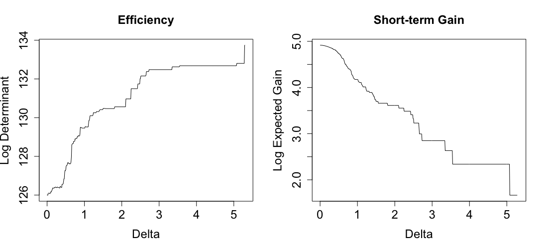
Figure 1 presents the efficiency/gain tradeoff as we vary the size of the randomization window in (8). For ease of visualization, we plot the logs of both quantities. As expected, we get a clear monotone increase in efficiency and decrease in gain as we increase , moving from an RDD to an RCT. It should be noted that our efficiency criterion, because it only uses information in the values, is robust to a poor choice of , whereas our gain definition is constrained by the assumption that is a reasonably accurate stand-in for the true treatment effect .
In practice, it is hard to interpret what a “good” value of efficiency is because of our D-optimality criterion. Hence, as in Owen and Varian (2020), a pragmatic approach is to first stipulate that the gain is at least some fraction of its highest possible value, and then pick the largest for this choice to maximize efficiency. A more qualitative choice based on results like Figure 1, such as picking the right endpoint of a sharp efficiency jump or the left endpoint of a sharp gain decline, would also be sensible.
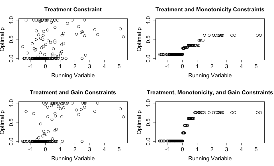
As we see in Figure 2, the treatment constraint causes most to be at or near zero or one. Adding the gain constraint pushes most of the treatment probabilities to zero for low values of the running variable and one for high values. This scenario most closely resembles the RDD, with some deviations to boost efficiency. Indeed, the optimal solution would necessarily tend towards the RDD solution as the gain constraint increased. Finally, the monotonicity constraint further pushes the higher values of to the positive values of the running variable and vice-versa, since we lose the opportunity to counterbalance some high and low probabilities at the extreme with their opposites. The right two panels display a few discrete levels in the treatment probability, consistent with Theorem 5.
7 Discussion
In this paper, we add to a growing body of work demonstrating the benefits of tie-breaker designs. Though RCTs are often infeasible, opportunities for small doses of randomization may present themselves in a wide variety of real-world settings, in which case treatment effects can be learned more efficiently. This phenomenon is analogous to similar causal inference findings about merging observational and experimental data (Rosenman et al., 2021, 2023; Colnet et al., 2024).
The convex optimization framework in Section 5 is more general and conveniently only relies on knowing sample data rather than population parameters. It is also simple to implement and allows one to incorporate natural economic and ethical constraints with ease.
Multivariate tie-breaker designs are a natural option in situations in which there is no clear univariate running variable. For example, subjects may possess a vector of covariates, many of which could be associated with heterogeneous treatment effects in some unknown way of interest. Of course, two-line models and their multivariate analogs are not nearly as complicated as many of the models found in practice. Our view is to use them as a working model by which to decide on treatment allocations, in which case a more flexible model could be used upon full data acquisition as appropriate.
8 Acknowledgements
We thank John Cherian, Anav Sood, Harrison Li and Dan Kluger for helpful discussions. We also thank Balasubramanian Narasimhan for helpful input on the convex optimization problem, Michael Baiocchi and Minh Nguyen of the Stanford School of Medicine for discussions about triage to hospital intensive care units, and an anonymous reviewer for helpful comments. This work was supported by the NSF under grants IIS-1837931 and DMS-2152780. T. M. is supported by a B. C. and E. J. Eaves Stanford Graduate Fellowship.
References
- Aiken et al. (1998) L. Aiken, S. West, D. Schwalm, J. Carroll, and C. Hsiung. Comparison of a randomized and two quasi-experimental designs in a single outcome evaluation: Efficacy of a university-level remedial writing program. Evaluation Review, 22(2):207–244, 1998.
- Angrist et al. (2014) J. Angrist, S. Hudson, and A. Pallais. Leveling up: Early results from a randomized evaluation of post-secondary aid. Technical report, National Bureau of Economic Research, 2014. URL http://www.nber.org/papers/w20800.pdf.
- ApS (2022) MOSEK ApS. MOSEK Fusion API for Python 9.3.18., 2022. URL https://docs.mosek.com/latest/rmosek/index.html.
- Atkinson et al. (2007) A. Atkinson, A. Donev, and R. Tobias. Optimum experimental designs, with SAS, volume 34 of Oxford Statistical Science Series. Oxford University Press, Oxford, 2007.
- Boruch (1975) R. F. Boruch. Coupling randomized experiments and approximations to experiments in social program evaluation. Sociological Methods & Research, 4(1):31–53, 1975.
- Boyd and Vandenberghe (2004) S. Boyd and L. Vandenberghe. Convex Optimization. Cambridge University Press, Cambridge, 2004.
- Bu et al. (2020) X. Bu, D. Majumdar, and J. Yang. D-optimal designs for multinomial logistic models. The Annals of Statistics, 48(2):pp. 983–1000, 2020.
- Campbell (1969) D. T. Campbell. Reforms as experiments. American psychologist, 24(4):409, 1969.
- Cappelleri et al. (1994) J. C. Cappelleri, R. B. Darlington, and W. M. K. Trochim. Power analysis of cutoff-based randomized clinical trials. Evaluation Review, 18(2):141–152, 1994.
- Cattaneo and Titiunik (2022) M. D. Cattaneo and R. Titiunik. Regression discontinuity designs. Annual Review of Economics, 14:821–851, 2022.
- Chaloner and Verdinelli (1995) K. Chaloner and I. Verdinelli. Bayesian experimental design: A review. Statistical Science, pages 273–304, 1995.
- Chang et al. (2017) D. Chang, D. Dacosta, and M. Shapiro. Priority levels in medical intensive care at an academic public hospital. JAMA Intern Med., 177(2):280–281, 2017.
- Colnet et al. (2024) B. Colnet, I. Mayer, G. Chen, A. Dieng, R. Li, G. Varoquaux, J.-P. Vert, J. Josse, and S. Yang. Causal inference methods for combining randomized trials and observational studies: a review. Statistical science, 39(1):165–191, 2024.
- Cook and Fedorov (1995) D. Cook and V. Fedorov. Constrained optimization of experimental design. Statistics, 26(2):129–148, 1995.
- Cook and Thibodeau (1980) R. D. Cook and L. Thibodeau. Marginally restricted d-optimal designs. Journal of the American Statistical Association, pages 366–371, 1980.
- Dette (1996) H. Dette. A note on bayesian c- and d-optimal designs in nonlinear regression models. The Annals of Statistics, 24(3):1225–1234, 1996.
- Fu et al. (2020) A. Fu, N. Balasubramanian, and S. Boyd. CVXR: An R package for disciplined convex optimization. Journal of Statistical Software, 94(14):1–34, 2020. doi: 10.18637/jss.v094.i14.
- Gelman and Imbens (2019) A. Gelman and G. Imbens. Why high-order polynomials should not be used in regression discontinuity designs. Journal of Business & Economic Statistics, 37(3):447–456, 2019.
- Gelman et al. (2020) A. Gelman, J. Hill, and A. Vehtari. Regression and other stories. Cambridge University Press, 2020.
- Goldberger (1972) A. Goldberger. Selection bias in evaluating treatment effects: Some formal illustrations. Technical report discussion paper, Institute for Research on Poverty, University of Wisconsin–Madison, 1972.
- Goldberger et al. (2000) A. L. Goldberger, L. A. N. Amaral, L. Glass, J. M. Hausdorff, P. Ch. Ivanov, R. G. Mark, J. E. Mietus, G. B. Moody, C.-K. Peng, and H. E. Stanley. Physiobank, PhysioToolkit, and PhysioNet: Components of a new research resource for complex physiologic signals. Circulation, 101(23):e215–e220, 2000.
- Hahn et al. (2001) J. Hahn, P. Todd, and W. Van der Klaauw. Identification and estimation of treatment effects with a regression-discontinuity design. Econometrica, 69(1):201–209, 2001.
- Heavlin and Finnegan (1998) W. D. Heavlin and G. P. Finnegan. Columnwise construction of response surface designs. Statistica Sinica, pages 185–206, 1998.
- Jacob et al. (2012) R. Jacob, P. Zhu, M.-A. Somers, and H. Bloom. A practical guide to regression discontinuity. Working paper, MDRC, 2012.
- Johnson et al. (2021) A. Johnson, L. Bulgarelli, T. Pollard, L. A. Celi, R. Mark, and S. Horng. MIMIC-IV-ED. https://doi.org/10.13026/77z6-9w59, 2021.
- Kluger and Owen (2023) D. M. Kluger and A. B. Owen. Kernel regression analysis of tie-breaker designs. Electronic Journal of Statistics, 17:243–290, 2023.
- Krantz (2022) C. Krantz. Modeling the outcomes of a longitudinal tie-breaker regression discontinuity design to assess an in-home training program for families at risk of child abuse and neglect. PhD thesis, University of Oklahoma, 2022.
- Kumar et al. (2018) S. Kumar, B. Shankar, S. Arya, M. Deb, and H. Chellani. Healthcare associated infections in neonatal intensive care unit and its correlation with environmental surveillance. Journal of Infection and Public Health, 11(2):275–279, 2018.
- Li and Owen (2022) H. Li and A. B. Owen. A general characterization of optimality in tie-breaker designs. Technical Report arXiv2202.12511, Stanford University, 2022.
- Li and Owen (2023) H. Li and A. B. Owen. A general characterization of optimality in tie-breaker designs. The Annals of Statistics, 51(3):1030–1057, 2023.
- Lipsey et al. (1981) M. W. Lipsey, D. S. Cordray, and D. E. Berger. Evaluation of a juvenile diversion program: Using multiple lines of evidence. Evaluation Review, 5(3):283–306, 1981.
- Lopez-Fidalgo and Garcet-Rodriguez (2004) J. Lopez-Fidalgo and S. A. Garcet-Rodriguez. Optimal experimental designs when some independent variables are not subject to control. Journal of the American Statistical Association, 99(468):1190–1199, 2004.
- Metelkina and Pronzato (2017) A. Metelkina and L. Pronzato. Information-regret compromise in covariate-adaptive treatment allocation. The Annals of Statistics, 45 (5):2046–2073, 2017.
- Morrison et al. (2024) Tim Morrison, Minh Nguyen, Michael Baiocchi, and Art B Owen. Constrained design of a binary instrument in a partially linear model. Technical report, arXiv:2406.05592, 2024.
- Nachtsheim (1989) C. J. Nachtsheim. On the design of experiments in the presence of fixed covariates. Journal of Statistical Planning and Inference, 22(2):203–212, 1989.
- Owen and Varian (2020) A. B. Owen and H. Varian. Optimizing the tie-breaker regression discontinuity design. Electronic Journal of Statistics, 14(2):4004–4027, 2020. doi: 10.1214/20-EJS1765. URL https://doi.org/10.1214/20-EJS1765.
- Phua et al. (2020) J. Phua, M. Hashmi, and R. Haniffa. ICU beds: less is more? Not sure. Intensive Care Med., 46:1600–1602, 2020.
- Rosenman et al. (2021) E. T. R. Rosenman, M. Baiocchi, H. Banack, and A. B. Owen. Propensity score methods for merging observational and experimental datasets. Statistics in Medicine, 2021.
- Rosenman et al. (2023) E. T. R. Rosenman, G. Basse, A. B. Owen, and M. Baiocchi. Combining observational and experimental datasets using shrinkage estimators. Biometrics, 79(4):2961–2973, 2023.
- Sagnol and Harman (2015) G. Sagnol and R. Harman. Computing exact -optimal designs by mixed integer second-order cone programming. The Annals of Statistics, 43(5):2198–2224, 2015.
- Slivkins (2019) A. Slivkins. Introduction to multi-armed bandits. Foundations and Trends in Machine Learning, 12(1–2):1–286, 2019.
- Vranas et al. (2018) K. Vranas, J. Jopling, J. Scott, O. Badawi, M. Harhay, C. Slatore, M. Ramsey, M. Breslow, A. Milstein, and M. Kerlin. The association of ICU acuity with outcomes of patients at low risk of dying. Crit Care Med., 46(3):347–353, 2018.
- Yang et al. (2016) J. Yang, A. Mandal, and D. Majumdar. Optimal designs for factorial experiments with binary response. Statistica Sinica, 26(1):385–411, 2016.
- Yang et al. (2017) J. Yang, L. Tong, and A. Mandal. D-optimal designs with ordered categorical data. Statistica Sinica, 27(4):1879–1902, 2017.
Appendix A Proofs
Proof of Theorem 2.
Using from (7), we have
where is symmetric and positive semi-definite. Now with equality if and only if , which occurs if and only if . Therefore, any design giving is prospectively D-optimal. From the formula (6) for , we see right away that the RCT satisfies this, which proves the first half of the theorem.
If we restrict to designs of the form (3), then for general we have
where . Consider a tuple for which . Then considering in particular the entry of where (so that ), we must have
| (19) |
where , , and . If we freeze and vary from to , we obtain
for all . Taking a suitable linear combination gives
Let , and analogously for and . Then
| (20) |
Next, equations (19) and (20) give respectively that
i.e., that
By definition, , so the left-hand side is non-negative and is negative. This implies that . Similarly, we have
and so
Therefore , and so . This leaves three possibilities: , , or both. If , then (19) implies that , which is impossible given (20). So then it must be that , whereupon (19) again implies that and (20) forces . In summary, a prospectively D-optimal design must satisfy
Proof of Theorem 3.
Let . The off-diagonal block matrix in (7) can now be written as
That is, we can write , where is as in (9) and has entry equal to . Note that is block diagonal, the exact opposite of . Let
| (21) |
To prove the theorem, we will simply show that and for , implying that (i.e., ) is the global maximizer of on this interval. Let
| (22) |
so that . Call a block matrix “block off-diagonal” if it is zero in the top-left entry and zero in the bottom-right block, as in the case of . The product of two block off-diagonal matrices is block-diagonal (with blocks of size and ), and the product of a block off-diagonal matrix and such a block diagonal matrix is block off-diagonal. Thus, and are both block diagonal, whereas is block off-diagonal. Differentiating , we obtain
so that . As noted, is block diagonal and is block off-diagonal, so the product is block off-diagonal and thus . It simplifies some expressions to let and . Then and
For , is the upper-left block of the inverse of the covariance matrix in (7), so it is positive semi-definite. Then is positive semi-definite as well and thus
In addition, is negative semi-definite, so
Therefore, everywhere, so is in fact a global optimum.
If , then and are both nonzero, so these two trace inequalities are strict. Then for all , so cannot be constant anywhere. Since is also concave on , the local optimum at must be a global optimum on this interval. ∎
Proof of Theorem 4.
To prove Theorem 4, we begin with two lemmas. We write for the probability density function. We start our study of efficiency by finding an expression for .
Lemma 1.
Proof.
The result is easy if . Without loss of generality, assume that . Let and be the vectors in formed by removing the th component from the vectors and , respectively. Using ,
and applying it a second time along with symmetry of , we get
Now let and with . Then we get
Lemma 2.
Proof.
For the general case of , with any positive-definite matrix, we define and write . Then , and so
This reduces the problem to the case with replaced by , so we obtain
Proof of Theorem 5.
In the optimization problem (18), is a fixed permutation in corresponding to a monotonicity constraint, and so it is no loss of generality to take to be the identity and omit it. If or , then clearly the only solution is the constant vector (all treated or all control), so we ignore that case henceforth.
Because we aim to show that optimal solutions have constant levels in , it will be easier to reparametrize in terms of the increments and show sparsity, where we take . Letting
and , we can rewrite this problem as
| (25) | ||||
The first three constraints correspond to and the monotonicity condition, while the last constraint corresponds to . Let be the vector with , so that the last constraint in (25) is . Moreover, let
so that the inequality constraints can be written simply as . Slater’s condition holds by considering the interior point
for any sufficiently small, so the KKT conditions are both necessary and sufficient. The Lagrangian is
where is a column vector formed from the ’th row of . The differential is then
Here, is the off-diagonal block of , which is symmetric since the off-diagonal block of itself is symmetric.
The stationarity condition is that the partial derivative above is zero for all . Suppose first that, for the optimal , {} are all nonzero, where is thus far unspecified. Later, we relax the condition that it is the first components of specifically that are nonzero.
The complementary slackness condition implies that for all , so in order for this to hold we must have . The stationarity condition for these terms is then
| (26) |
The right-hand side of (26) is linear in , with slope and intercept that depend on and . These constitute two free parameters on the right-hand side. For a fixed matrix , this is therefore a probability zero event whenever , since are sampled IID from a density. However, the issue here is that is not fixed but rather an implicit function of the data matrix . Thus, we instead show that, for sufficiently large and with probability one, there is no symmetric matrix and pair with
| (27) |
Here, the logic is analogous: there are free parameters for an arbitrary symmetric matrix , as well as two additional parameters from and . Thus, if , this cannot happen with probability one. The logic is the same for any size subset of , not just the first , so the result follows by a union bound.
∎