Multiscale Solar Wind Turbulence Properties inside and near Switchbacks measured by Parker Solar Probe
Abstract
Parker Solar Probe (PSP) routinely observes magnetic field deflections in the solar wind at distances less than 0.3 au from the Sun. These deflections are related to structures commonly called ’switchbacks’ (SBs), whose origins and characteristic properties are currently debated. Here, we use a database of visually selected SB intervals—and regions of solar wind plasma measured just before and after each SB—to examine plasma parameters, turbulent spectra from inertial to dissipation scales, and intermittency effects in these intervals. We find that many features, such as perpendicular stochastic heating rates and turbulence spectral slopes are fairly similar inside and outside of SBs. However, important kinetic properties, such as the characteristic break scale between the inertial to dissipation ranges differ inside and outside these intervals, as does the level of intermittency, which is notably enhanced inside SBs and in their close proximity, most likely due to magnetic field and velocity shears observed at the edges. We conclude that the plasma inside and outside of a SB, in most of the observed cases, belongs to the same stream, and that the evolution of these structures is most likely regulated by kinetic processes, which dominate small scale structures at the SB edges.
1 Introduction
Parker Solar Probe (PSP) is the first mission to measure the inner heliosphere closer than 0.3 au from the Sun’s surface, with perihelion distances of 0.16 au during its first three encounters with the Sun. One of the most compelling results from these first encounters is the ubiquity of so-called ’switchback’ structures (SBs)111These structures are also called ’spikes’, ’jets’ or ’magnetic field reversals’ in the literature., characterized by a rotation of the magnetic field observed by the spacecraft (Kasper et al., 2019; Bale et al., 2019). Along with the magnetic field rotation, the magnitude of the solar wind bulk velocity increases by the order of the local Alfvén speed (Matteini et al., 2014), where is magnetic permeability of vacuum, and and are proton density and mass, respectively. Results from previous missions had already motivated the community to invest significant effort into understanding the nature of SBs, though they were not observed nearly as frequently as by PSP. Now, this interest has increased, as new data sets from PSP provide significantly larger populations of SBs and more detailed information on the associated plasma and electromagnetic field conditions due to increased measurement precision and cadence.
1.1 Previous observations of Switchbacks in the solar wind
The first observations of sudden magnetic field rotations were reported in Pioneer 6 observations (Burlaga, 1969, 1971), and later in Helios measurements (Marsch et al., 1981). A decade later, measurements from the Ulysses mission confirmed that the probability distributions of the magnetic field orientation are not uniform, but are rather skewed toward the polarity opposite to the dominant polarity of the solar hemisphere the spacecraft was observing (Forsyth et al., 1995). This result was followed by a statistical analysis of Ulysses high latitude observations (McComas et al., 1998) that demonstrated the opposite polarity measurements occurred in a non-negligible () fraction of observations, but only a minor fraction (of the order of a percent) of these featured a complete inversion of the magnetic field (Balogh et al., 1999). These events were classified as discontinuities—either tangential discontinuities (TD), usually separating two different plasma streams; or rotational discontinuities (RD), with a single stream following a folded magnetic field line (Burlaga et al., 1977; Neubauer & Barnstorf, 1981). Applying the standard Minimum Variance Analysis (MVA) procedure (see e.g. Sonnerup & Scheible (1998)), to single-point measurements (Burlaga & Ness, 1969; Mariani et al., 1973; Smith, 1973; Neugebauer et al., 1984; Lepping & Behannon, 1986), RDs are more frequently observed than TDs. In contrast, analysis of sets of manually selected events simultaneously observed by three different spacecraft at 1 au (Tsurutani & Smith, 1979; Horbury et al., 2001), and shortly after of four-point measurements from the Cluster II mission (Knetter et al., 2003, 2004), found TDs to be dominant. These authors argued that results derived from MVA might be misleading due to presence of surface waves on TDs (Denskat & Burlaga, 1977; Hollweg, 1982), and therefore observations of magnetic field folds manifest in RDs are not as common as initial work suggested.
Although there is an evident ambiguity in the identification of SBs, they were considered to be isolated events (Horbury et al., 2001; Yamauchi et al., 2004; Horbury et al., 2018) that had been studied in detail with some basic properties well established prior to the launch of PSP. It was understood that the magnetic field deflection in SBs is followed by both the proton (Neugebauer & Goldstein, 2013) and electron beam (also known as the strahl) (Kahler et al., 1996). Similar behavior was observed for relative drift between proton and particle populations (Yamauchi et al., 2004). The fluctuations of the magnetic and velocity field at large scales, meaning the scales in the MHD domain with size comparable to the size of a structure, are linearly related, describing a dominantly Alfvénic turbulence (Gosling et al., 2009). Moreover, it can be shown that the SB magnetic and velocity fluctuations are spherically polarized in the reference frame of zero electric field (Gosling et al., 2011; Matteini et al., 2014), which can be well approximated by the particle’s velocity, due to their weak interaction with Alfvénic fluctuations of protons (Matteini et al., 2015). Some turbulent properties, e.g. power spectra and cascade rates, are found to be very similar inside and outside of SBs, though discrete changes of velocity and the magnetic field are contributing to intermittency of turbulence within observed events (Horbury et al., 2018).
Starting with the first PSP solar encounter in November 2018, a plethora of new results regarding SBs were reported, as these structures were consistently observed and resolved with high resolution measurements for radial distances less than 0.25 au. These first results provided an overview of SB properties, finding some differences compared to previous reports. Most notably, PSP did not observe SBs as isolated events, but rather ’clustered’ phenomena (Dudok de Wit et al., 2020), with measured parallel temperature changing as the spacecraft moves through the cluster (Woodham et al., 2020). This claim is supported by two independent arguments: 1) normalized magnetic field deflections from the Parker spiral (scaled to values between 0 and 1 depending on cosine value) exhibit a power law distribution, which is a property related to phenomena such as entangled filaments and flux tubes, rather than a Gaussian distribution, which would represent randomized events; and 2) Detrended Fluctuation Analysis (Kantelhardt et al., 2001) shows an increase in long range correlations in time series for SBs compared to quiescent intervals. These ’clusters’ are found to be separated by quiet periods with few SBs (Horbury et al., 2020). The origin of this discrepancy between PSP and previous measurements is not easy to understand due to PSP’s unique trajectories compared to previous missions, nearly co-rotating with the Sun’s surface during significant fractions of its first encounters (Bale et al., 2019; Badman et al., 2020a; Rouillard et al., 2020). This specific trajectory is likely causing the observed magnetic field deflections to have shorter duration in measurements for larger radial distance, as the spacecraft could be slicing through an elongated structure, possibly aligned along the Parker spiral (Laker et al., 2020). Apart from these unexpected characteristics, many similarities between PSP and previous SB observations remain. First, SBs are found to be dominantly Alfvénic structures, with direction of Poynting flux and turbulent fluctuations changing along with the magnetic field (McManus et al., 2020; Bourouaine et al., 2020; Mozer et al., 2020), maintaining the correlation between bulk velocity and magnetic field when the field is inverted (Matteini et al., 2014), while proton temperature does not vary significantly through sharp field reversals (Wooley et al., 2020). Second, Mozer et al. (2020) found that that the Poynting flux remains conserved before and after a SB, but significantly increases inside the structure. Third, the Partial Variance of Increments (PVI) of the magnetic field, a proxy for intermittency, is also found to be increased in clustered intervals (Chhiber et al., 2020), in accordance with previous results. Finally, it is worth emphasizing that a very careful case study by Krasnoselskikh et al. (2020) demonstrated that not all SBs appear to be Alfvénic in nature. Some of the events exhibit significant wave activity, especially at the borders of SBs. This is consistent with signatures of current sheets (Farrell et al., 2020) and Whistler modes (Agapitov et al., 2020), detected at the edges of these structures, where the magnetic field is rotating.
1.2 A Mystery of Switchback Origins
The characteristics of SBs listed in Section 1.1 do not conclusively demonstrate how SB are formed or how they evolve throughout the inner heliosphere. Proposed mechanisms for the creation of SBs can be roughly classified in two groups - they either form on or very close to the solar surface, or are generated in the propagating solar wind - with both interpretations being represented in the literature.
A connection between SB characteristics and surface source structures could lend credence to the theories suggest SBs form on or close to the surface of the Sun. Toward this end, many authors have investigated the connection between the plasma streams of increased bulk velocity and coronal jets (McComas et al., 1995; Neugebauer et al., 1995; Culhane et al., 2007; Patsourakos et al., 2008; Neugebauer, 2012; Tian et al., 2014)222For an extensive review of the remote sensing observations of interest, see Raouafi et al. (2016).. Since the Alfvénic fluctuations in the chromosphere contain a significant amount of energy (De Pontieu et al., 2007), one possible interpretation of our in situ observations, also supported by extensive simulation work (Uritsky et al., 2017; Wyper et al., 2017; Roberts et al., 2018), is that these fluctuations will continue to propagate even if a jet does not escape the Sun’s gravity (Horbury et al., 2020). Another candidate mechanism is interchange reconnection, which arises from magnetic flux transport close to the surface through structures such as coronal loops (van Ballegooijen et al., 1998; Fisk & Schwadron, 2001; Fisk, 2005), interacting with open magnetic field lines to create S-shaped structure observed as a SB (Fisk & Kasper, 2020; Zank et al., 2020). Recent MHD simulations show that, if a SB is in equilibrium with the surrounding plasma, it can preserve its shape long enough to reach PSP (Landi et al., 2005; Tenerani et al., 2020). Further on, it is expected to gradually merge with the surrounding plasma, most likely via parametric decay instability (Derby, 1978), a process potentially at work in the solar wind, as observed on Wind mission (Bowen et al., 2018a), and predicted by turbulence models (Chandran, 2018), hybrid (Matteini et al., 2010) and MHD simulations (Tenerani & Velli, 2013; Primavera et al., 2019).
The complementary argument is that magnetic field folds are generated as the solar wind propagates. The main observational support for this argument is that the fraction of the solar wind with inverted magnetic field increases with radial distance (Forsyth et al., 1995; McComas et al., 1998; Borovsky, 2016; Owens et al., 2018; Macneil et al., 2020; Badman et al., 2020b). Also, simulations non-compressible three dimensional MHD turbulence (Zhdankin et al., 2012) show that measured the distribution of magnetic field orientation at 1 au can be caused solely by turbulent fluctuations. Although these studies provide information on the statistics of the magnetic field and electron strahl orientation, more detailed research of strictly defined SBs, their duration, deflection angles and other parameters for purposes of effective comparison with PSP results has yet to be performed. Regarding possible mechanisms for the generation of magnetic field reversals as the solar wind propagates outwards, MHD simulations show that they can develop from velocity shears (Landi et al., 2006; Ruffolo et al., 2020). SBs are predicted to appear as a product of turbulent fluctuations evolving while maintaining constant magnetic field intensity (Vasquez & Hollweg, 1996). The discontinuity, which forms due to the fact that a three dimensional configuration for which the field fluctuation is of the order of the field intensity is not expected to be possible (Barnes, 1976; Valentini et al., 2019), creates the observational signature such the one observed by PSP (Squire et al., 2020). It is important to note that, even if the role of the turbulent cascade turns out not to be crucial for SB generation, the effects of turbulent fluctuations on SB evolution needs to be investigated in detail (Chen et al., 2020).
1.3 Outline of the paper
Having reviewed previous observational results related to SBs and associated physical interpretations, we will now move to our analysis of SBs observed by PSP during encounters 1 and 2. The intention of this work is not to verify or disprove either school of thought regarding SB origins described in Section 1.2, but rather to analyze a set of observations that have the combined benefit of both being visually selected and also containing a large number of events, which will provide additional insight into both MHD and kinetic scale properties of SBs. This way, the results presented here provide a comprehensive set of observational constraints for current, as well as developing future models of SB generation and evolution.
We use a database of visually selected SBs, with associated quiet and transition periods before and after each structure. For each event, we combine several methods to analyze plasma parameters, turbulent spectra, and intermittency levels. Additionally, as a proxy for turbulence behavior at ion scales, we compare levels of Stochastic Heating (SH), a non-linear plasma heating mechanism based on the breaking of magnetic moment by low-frequency turbulent fluctuations at ion scales (Chandran et al., 2010), inside and outside of SBs. Details of these procedures are described in Section 2. In Section 3, we review our results and discuss possible implications. Finally, Section 4 summarizes the main points.
2 Method
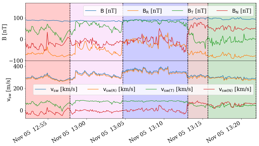
Within the heliospheric community, the exact definition and typical properties of SBs are still debated. Several different criteria to identify SBs in data sets have been introduced throughout the last few decades (Yamauchi et al., 2004; Horbury et al., 2018) and in particular in studies related to PSP data (Dudok de Wit et al., 2020; Horbury et al., 2020; McManus et al., 2020; Mozer et al., 2020; Bourouaine et al., 2020). Here, we use the database of SBs from PSP Encounters 1 and 2 (E1 and E2) where, for each event, five separate regions are identified: 1) Leading Quiet Region (LQR) with stable velocities and magnetic fields before the SB; 2) Leading Transition Region (LTR), where the magnetic field rotates from LQR toward its SB orientation; 3) the SB itself with stable field orientation; 4) Trailing Transition Region (TTR); and 5) Trailing Quiet Region (TQR), with conditions which are, in general, not very different from the ones in LQR. The identification of events was done through visual inspections of and time series. Magnetic field rotations coincident with the bulk velocity enhancement are selected, with the results being very consistent throughout multiple independent manual inspections. A total of 1,074 events333Further on, the term ’event’ will be used for a sequence of the five different observed regions, while the term ’SB’ will be used only for the period where the rotated magnetic field is observed. were identified (662 in E1 and 412 in E2), 921 of which have all five distinct regions resolved. A typical example of a selected event is given on Figure 1. For each of these regions separately, we extracted the average plasma parameters, including the proton core population density , thermal velocity and solar wind bulk velocity from the Solar Probe Cup (SPC) measurements (Kasper et al., 2016; Case et al., 2020), magnetic field from the Fields instrument suite magnetometers (Bale et al., 2016) and temperatures perpendicular and parallel to from analysis of effective temperatures measured by SPC and the fluctuating magnetic field (Huang et al., 2020a). Only measurements flagged with the highest degree of confidence by the instrument teams are used in this study.
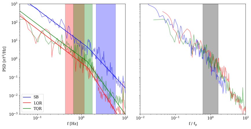
We also calculate the Fourier magnetic field trace Power Spectral Density (PSD) spectrum444For details on calculating PSD, see e.g. Appendix A of Bourouaine & Chandran (2013). for each region, focusing on two characteristic regimes: 1) the inertial range where the Alfvénic fluctuations cascade toward smaller scales, characterized by a logarithmic scale slope usually measured in the domain [-1.7, -1.45] (Bruno & Carbone, 2013) and, after the spectral break frequency , 2) the kinetic range where the fluctuations both become dispersive and the energy in the electromagnetic field is expected to more efficiently dissipate, eventually leading to plasma heating, causing significant steepening of the spectral slope (Alexandrova et al., 2012; Verscharen et al., 2019)555This is a very simplified description of a typical turbulent spectrum. The border between the two described spectral regions is often observed as a third range at which the spectral steepening is associated with ion heating through kinetic processes (Sahraoui et al., 2010; Bowen et al., 2020).. As multiple other phenomena, such as coherent structures likely generated by turbulence (Lion et al., 2016; Howes, 2016), magnetic reconnection (Mallet et al., 2017; Loureiro & Boldyrev, 2017; Vech et al., 2018), or instrument noise (Martinović et al., 2019) can interfere with measuring the background turbulent spectra, and as the event durations vary significantly, we calculated the spectral indices and the PSD at the ion scale break using a two step process. First, a Levenberg-Marquardt fit using a two line function, with the fitting range frequencies set manually assuring that both injection range and instruments noise are excluded, is performed for each LQR, SB and TQR region for a given event. This method provided results for the spectral break locations and PSD intensities with high accuracy and independent of initial guess and input parameters, but introduced a subjective bias on the values of inertial range logarithmic slopes through the manual selection of the low frequency limit. Therefore, the second step of the fitting algorithm was determining the inertial slopes by a least-square line fit of data in an automatically selected range. To avoid statistical uncertainties and the possible measurements of the injection range turbulence, the low frequency limit was set at 150% of the minimum frequency of the power spectrum of a given region, while the high frequency limit was set at , to avoid sampling the fine structure of the spectral break. An example of such a fit is given on Figure 2. We see both LQR and TQR spectra encounter the noise floor at 6 Hz. The frequency range contaminated by the noise is manually removed from the fitting procedure as to not affect the resulting slopes. In total, spectra from 1,863 regions (LQRs, SBs and TQRs) were fit successfully, and are included in this study.
It is worth emphasizing that a significant increase of in SBs causes a shift of the spectrum in frequency space, in accordance with the shift prescribed by Taylor hypothesis (Taylor, 1938). The Right panel of Fig. 2 illustrates this property, with the three spectra, fairly different in terms of measured power, overlap as the observed frequency is normalized to . Here, is the convected gyrofrequency (Bourouaine & Chandran, 2013), is the angle between and B, is the gyroradius, and is the elementary charge with all values averaged over a measured region.
As the magnetic field PSD does not capture the intermittent properties of turbulence, including phenomena such as localized coherent structures at the borders of the regions within each event, we estimate these properties using PVI, which is defined at time for some time increment as
| (1) |
where , denotes ensemble average over a region of interest (QR, TR or SB). Based on previous studies, times with values of PVI 3 have been associated with non-Gaussian structures, events with PVI 6 categorized as current sheets, and with PVI 8 as reconnection sites (Matthaeus & Goldstein, 1982; Osman et al., 2012; Greco et al., 2018; Chhiber et al., 2020).
Detailed analysis of the turbulent spectra around provides estimates of ion heating delivered through non-linear mechanisms such as stochastic heating (SH). An overview of estimates for SH rates for the first two PSP encounters is provided elsewhere (Martinović et al., 2020), while in this study we will only focus on the comparison of SH in SBs and their associated quiet regions. The key quantity for estimation of SH is the normalized level of turbulent magnetic fluctuations at the convective gyroscale , leading to a total heating rate estimated as (Hoppock et al., 2018)
| (2) |
where , , and are order unity constants found from test particle simulations that are expected to be fairly insensitive to plasma parameters (Chandran et al., 2010; Hoppock et al., 2018). The relation between velocity and magnetic field fluctuations is quantified by the parameter , proton cyclotron frequency is given as , and . A detailed discussion of these constants is beyond the scope of this work, but can be found in previous literature on SH in the solar wind (Chandran et al., 2010; Xia et al., 2013; Hoppock et al., 2018; Martinović et al., 2019). The magnetic field fluctuation magnitude at the convective gyroscale is calculated by integrating the PSD in the vicinity of , as shown on Figure 2)
| (3) |
In Equation 3, is the PSD logarithmic slope in the integration range, determining the geometrical factor , which is described in detail in previous studies (Bourouaine & Chandran, 2013; Vech et al., 2017). We note that SH rates determined this way have very large uncertainties (Martinović et al., 2019), but can be confidently used for comparison between different regions in a single event.
3 Results and Discussion
3.1 Overview of Plasma Parameters
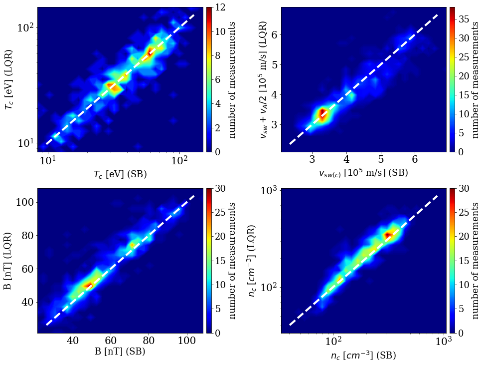
The macroscopic parameters of SBs and LQRs are shown in Figure 3. Magnetic field strength, core proton density and temperature666The SPC data set does not provide full values of temperature, but rather ones extracted from the reduced distributions. The scalar used here is provided by method described in (Huang et al., 2020a)., as well as other parameters which are not shown, are fairly similar inside and outside of SBs for the vast majority of events. The two peaks along the diagonal appearing in all three plots are due to the combination of data sets from E1 and E2, which have slightly different typical parameters. This is also the case for comparison between SBs and TQRs, not shown. These observations agree with the interpretation that plasma inside SBs is from the same folded plasma stream as the quiet regions outside the SB (see, e.g. (Yamauchi et al., 2004; Tenerani et al., 2020; Fisk & Kasper, 2020; Wooley et al., 2020)). However, it is not intuitively clear why the bulk velocity should increase by within SBs. Even though the deflection angle777In this work, deflection angle is defined as the difference in average between LQR and SB for each event. The differences between TQR and SB are consistent to within several percent for large majority of events. of the bulk velocity for SBs is very small (Kasper et al., 2019), we find that the intensity of the has a Gaussian distribution centered at (not shown). This value does not necessarily conflict with previous results, which argue that magnetic field deflections in SBs behave like almost purely Alfvénic phenomenon (Yamauchi et al., 2004; Gosling et al., 2011; Matteini et al., 2015; Horbury et al., 2018), as these values are not comparing the states just before and after the transition regions, but are rather averaged over longer periods. One possible interpretation for such behavior is that the difference in bulk speeds, normalized to Alfvén speed, is proportional to the Alfvénic ratio between energy of magnetic field and velocity fluctuations, expected to be lower than unity in the solar wind (Matteini et al., 2014), but this phenomena requires additional detailed investigation.
3.2 Turbulence
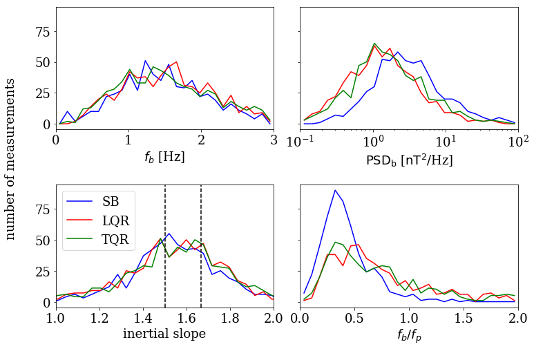
Figure 4 shows the results from 1,863 manually fitted turbulent spectra in SBs and quiet regions. The most notable feature is that, even though the turbulent spectra are shifted in frequency due to increased , the spectral break from inertial to ion dissipation region spans the same frequency range. This implies the lowest wavenumber at which the dissipation is observed is lower in SBs, producing larger power at the break point (top panels). Bottom right panel shows comparison of the spectral break point with the convective gyroscale, also shifted toward higher frequencies (Figure 2), which is due to the increase in both and , given that all the other quantities comprising do not significantly change inside SBs (Figure 3). The relation of the convected proton inertial length to (not shown) is very similar, which is expected as our data set does not contain any extremely high or low plasma measurements, as studied for example in Chen et al. (2014). It is important to note the contrast with recent results (Duan et al., 2020) showing different scalings of and in PSP data; this difference is most likely masked in our results due to similarity in MHD plasma parameters in QRs and SBs (Figure 3).
The fitted values of inertial range turbulence slopes shown in the bottom left panel are consistent with two theoretically predicted regimes—a standard ’critically balanced’ cascade with inertial slope centered around -5/3 (Goldreich & Sridhar, 1995), and a ’dynamically aligned’ cascade with the inertial slope of (Boldyrev, 2006), describing a majority of the measured spectra with similar abundances in histograms. There is no preference to either of these regimes when comparing SBs to quiet regions. In order to understand the inertial slope behavior, we investigated possible relations of the fitted slope with multiple parameters, including plasma , Velocity Distribution Function (VDF) moments, magnetic field and characteristics of its turbulent fluctuations, and radial distance. None of these parameters showed a correlation with the inertial slope values. However, this result does not necessarily contradict with previous studies where the inertial slope was observed to depend on the residual energy and intermittency (Bowen et al., 2018b), cross helicity (Chen et al., 2013), radial distance (Chen et al., 2020), or proximity to the Heliospheric Current Sheet (Chen et al., 2021), due to relatively small ranges for these parameters measured in our data set. Similar studies to this work on the inertial slope dependencies will be preformed in the future as the PSP data set expands, producing larger numbers of visually identified SB for analysis.
3.3 Comparison of SH Rates
To investigate properties of the ion scale turbulence and its interaction with VDF moments, we estimate the level of non-linear SH. Here, it is important to note that the SH values are very difficult to estimate for majority of events due to their relatively short duration and occasional strong wave activity. Therefore, these estimates should be observed only as a proxy for behavior of turbulence at the proton gyroscale, and its comparison inside and outside of SBs. The SH rates measured on this mission are considered in more detail and with more strict constraints elsewhere (Martinović et al., 2020), while discussion of other solar wind heating mechanisms, such as Landau damping (Quataert, 1998; Chen et al., 2019) or cyclotron heating (Hollweg, 1999; Kasper et al., 2013), is beyond the scope of this paper.
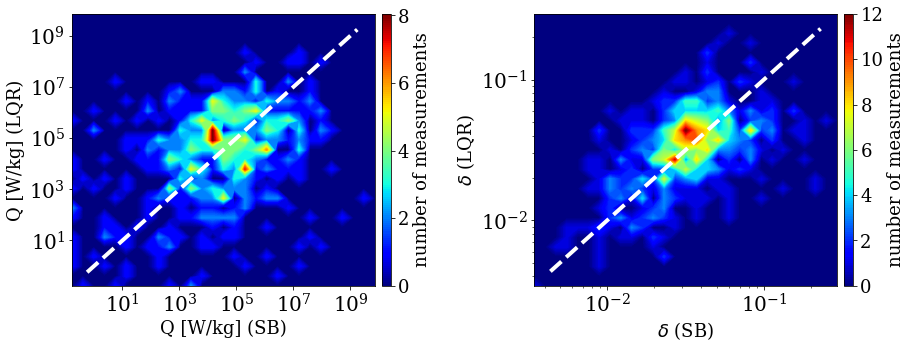
The turbulent PSD at the convective gyroscale is related to the level of SH through the value of , which is largely controlled by the amplitude of the PSD in the integration range around , defined in Equation 3. This range is, for most cases, closer to in quiet regions than in SBs (Figure 4). However, as the PSD at the break is significantly higher for SBs, the integration range levels, and consequently at the gyroscale, remain very similar, as shown on Figure 5. Considering that the parameters shown on Figure 3 are also very similar, the value of SH in SBs remains approximately the same and thus the existence of SBs is not expected to enhance the contribution of SH to solar wind heating. Observing Figure 2, we could argue that the similarity in the estimated SH values originates from the wave vector PSD, Doppler shifted to different frequencies. However, two important characteristics must be taken into account when considering SH rates — 1) the PSD at is increased for SBs and 2) the frequency of interest does not represent a standard Doppler shift, but is also affected by the angle , pushing the integration range to slightly higher frequencies. These two factors have effects that partially negate one another, providing to the level of accuracy available, similar values of SH rates.
3.4 Effects of Borders and Intermittency
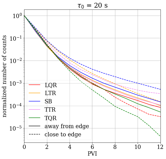
Similar characteristics of the turbulent spectra shown in Figure 4 do not reflect the potentially different intermittency levels in different regions. The distribution of PVI values, used as a proxy for intermittency, is shown on Figure 6 organized by the five kinds of regions, clearly demonstrating that PVI is the highest for the case of SBs, then TRs, and is the lowest for QRs (Huang et al., 2020b). As recent results (Krasnoselskikh et al., 2020; Agapitov et al., 2020; Farrell et al., 2020) have shown that the edges of SBs can be populated by various structures and exhibit strong wave activity, we separately observe the measurements close to the edges of each region. Solid lines are calculated using only PVI values measured at least s from the region’s edge. The histograms start to deviate for SB and transition regions for PVI = 3-6, with the difference of at PVI and for about a factor of 2.4 at PVI . On the other hand, the magnetic field sampled close to the region edges are featuring significantly more drastic trends, with spread of a factor of 2.3 for PVI , and over an order of magnitude for PVI . This result is insensitive to the used; recalculating Figure 6 with of 1, 2, 5, 10, and 50 s (not shown) yields very similar results. We also reproduced Figure 6, but only taking into account periods either larger or smaller than various time durations between 2 and 200 s. The results are very similar to the ones shown on the Figure, and are not displayed here. From here, we conclude that properties of PVI are independent of the region duration. This result is fully consistent with previous observations findings of SBs having increased intermittency (Horbury et al., 2018), as well as the presence of waves and enhanced currents at the edges of SBs. The presence of these structures at the SB borders suggests that they might be responsible for increased ’lifetime’ of SBs, stabilizing these structures against decay (Landi et al., 2005).
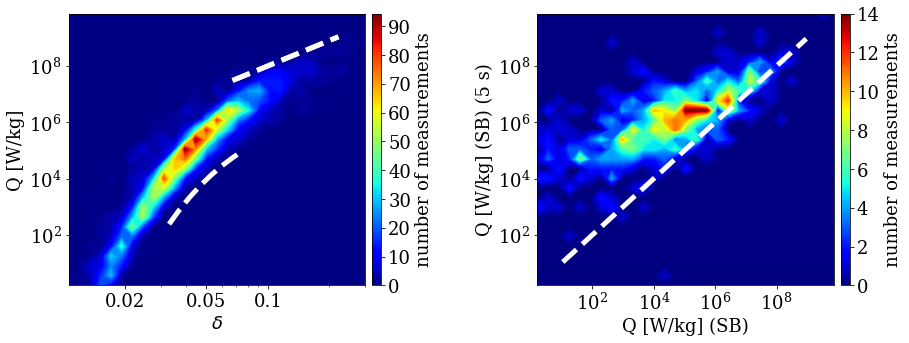
Finally, it is interesting to consider the effects of intermittency on SH. Figure 7 illustrates the SH values calculated for every 5 s interval and then averaged over the entire region. It is notable that the intermittency strongly enhances the level of SH whenever that level is low, but it is not the case for intervals with strong SH, which are responsible for the majority of SH’s contribution to solar wind heating (Martinović et al., 2019, 2020). This feature, shown on right panel of Figure 7, was verified to also hold for quiet regions and any time averages in [5-100] s range. To understand this effect, we refer to the work of Mallet et al. (2019), who calculated fluctuations damping rates for different solar wind heating mechanisms. Here, is the theoretical heating rate, and is the Elsasser variable (Elsasser, 1950) at a given scale. For the case of Landau damping, intermittency has no effect on the heating intensity due to the damping rate increasing linearly with . On the other hand, the SH was expected to be strongly affected by intermittency due to the exponential factor in Equation 2. However, the left panel shows that SH dependence on transitions from an exponential to a power law function. This implies that the damping rate for the case of SH is approaching the linear function as the exponential factor either approaches unity, becoming a very weak function of . Therefore, when SH is a very important, and possibly dominant, heating mechanism, its level and variance within SBs and quiet regions, are significantly less affected by intermittency compared to intervals when SH is low.
However, another level of analysis of this topic is related to the relation between intermittency and order unity constants , , and , given in Equation 2. Results of RMHD simulations (Xia et al., 2013) indicate that their predicted values can be notably decreased depending on the nature of the turbulent fluctuations, increasing the predicted SH rate. This topic requires separate detailed investigation which is outside of the scope of this paper.
4 Conclusion
In this work, a comprehensive analysis of manually selected magnetic field SB events in PSP encounters 1 and 2 is performed in order to determine the characteristics of plasma inside and outside of the regions where the field is deflected. The investigation shows that the plasma has very similar bulk quantities and magnetic field values inside SBs, compared to the equivalent values in the quiet regions before and after a SB, with the very well known shift in the solar wind bulk speed being of the order of the Alfvén speed. Additionally, estimates of the non-linear SH rates inside and outside SBs show that the heating rate due to this mechanism remains fairly similar, which suggests that the plasma sampled by the spacecraft in different regions of a single event most likely belong to a single plasma stream.
However, several questions are raised related to the turbulent cascade and kinetic processes in these events. First, the magnetic field power spectra ion-scale breaking frequency remains similar inside and outside of SBs, in spite of the spatial turbulent spectra in SBs being shifted toward higher frequencies due to effects of Taylor hypothesis. Second, we observed the inertial range PSD logarithmic slopes to have a distribution consistent with both the values of -5/3 and -3/2, characteristic for the classic critical balance and dynamic alignment turbulence theories, respectively. The inertial logarithmic slope is not sensitive to typical physical quantities such as density, pressures, or radial distance, and its phenomenology remains unclear, but this could be due to relatively limited range of the plasma parameters measured. Third, the increased values of PVI in the transition regions and SBs compared to quiet regions, with this property being independent of the region duration, reflects the existence of small scale structures at the region borders. The origin of these structures is directly related to the SB origins and will be one of the central questions regarding SB evolution in need of resolution.
In reference to the two different schools of thought about SB origins discussed in Section 1.2, the fact that we generally observe the same plasma inside and outside of what is most likely an S-shaped structure (Dudok de Wit et al., 2020; Horbury et al., 2020), implies that either 1) a parcel of solar wind plasma expands outwards until the turbulent fluctuations become sufficiently strong to fold magnetic field back on itself, forming a SB; or 2) the magnetic field structure travels through the solar wind with the relative speed of the order of , folding the plasma without significantly altering its internal structure. In the second scenario, complicated processes near the solar surface, such as interchange reconnection (see e.g. Fisk & Kasper (2020); Zank et al. (2020)), create a structure that persists as it propagates through the solar wind, temporarily increasing the speed of the part of the stream which is being pulled through the structure.
The transition regions and edges themselves are not investigated in detail in this work. Although the basic phenomenology of these regions is well understood, their comparison with quiet regions and SBs is not trivial, and the magnetic field PSD from these regions require a more sophisticated interpretation. The kinetic scale processes and ion-scale turbulence inside SBs, and development and dissipation of current sheets at their edges, remain an open topic for future effort. Finally, we note that all the remarks made in this paper are meant to describe characteristics of the majority of observed events, and therefore provide observational constraints for models aiming to describe SBs. We do not expect future case studies, which would cover single or few interesting events in more detail, to necessarily replicate all the general conclusions given here.
References
- Agapitov et al. (2020) Agapitov, O. V., Dudok de Wit, T., Mozer, F. S., et al. 2020, The Astrophysical Journal Letters, 891, L20
- Alexandrova et al. (2012) Alexandrova, O., Lacombe, C., Mangeney, A., Grappin, R., & Maksimovic, M. 2012, The Astrophysical Journal, 760, 121
- Badman et al. (2020a) Badman, S. T., Bale, S. D., Martínez Oliveros, J. C., et al. 2020a, The Astrophysical Journal Supplement Series, 246, 23
- Badman et al. (2020b) Badman, S. T., Bale, S. D., Rouillard, A. P., et al. 2020b, arXiv e-prints, arXiv:2009.06844
- Bale et al. (2016) Bale, S. D., Goetz, K., Harvey, P. R., et al. 2016, Space Science Reviews, 204, 49
- Bale et al. (2019) Bale, S. D., Badman, S. T., Bonnell, J. W., et al. 2019, Nature, 576, 237
- Balogh et al. (1999) Balogh, A., Forsyth, R. J., Lucek, E. A., Horbury, T. S., & Smith, E. J. 1999, Geophysical Research Letters, 26, 631
- Barnes (1976) Barnes, A. 1976, Journal of Geophysical Research, 81, 281
- Boldyrev (2006) Boldyrev, S. 2006, Physical Review Letters, 96, 115002
- Borovsky (2016) Borovsky, J. E. 2016, Journal of Geophysical Research (Space Physics), 121, 5055
- Bourouaine & Chandran (2013) Bourouaine, S., & Chandran, B. D. G. 2013, The Astrophysical Journal, 774, 96
- Bourouaine et al. (2020) Bourouaine, S., Perez, J. C., Klein, K. G., et al. 2020, The Astrophysical Journal Letters, 904, L30
- Bowen et al. (2018a) Bowen, T. A., Badman, S., Hellinger, P., & Bale, S. D. 2018a, The Astrophysical Journal Letters, 854, L33
- Bowen et al. (2018b) Bowen, T. A., Mallet, A., Bonnell, J. W., & Bale, S. D. 2018b, The Astrophysical Journal, 865, 45
- Bowen et al. (2020) Bowen, T. A., Mallet, A., Bale, S. D., et al. 2020, Physical Review Letters, 125, 025102
- Bruno & Carbone (2013) Bruno, R., & Carbone, V. 2013, Living Reviews in Solar Physics, 10, 2
- Burlaga (1969) Burlaga, L. F. 1969, Solar Physics, 7, 54
- Burlaga (1971) —. 1971, Journal of Geophysical Research, 76, 4360
- Burlaga et al. (1977) Burlaga, L. F., Lemaire, J. F., & Turner, J. M. 1977, Journal of Geophysical Research, 82, 3191
- Burlaga & Ness (1969) Burlaga, L. F., & Ness, N. F. 1969, Solar Physics, 9, 467
- Case et al. (2020) Case, A. W., Kasper, J. C., Stevens, M. L., et al. 2020, The Astrophysical Journal Supplement Series, 246, 43
- Chandran (2018) Chandran, B. D. G. 2018, Journal of Plasma Physics, 84, 905840106
- Chandran et al. (2010) Chandran, B. D. G., Li, B., Rogers, B. N., Quataert, E., & Germaschewski, K. 2010, The Astrophysical Journal, 720, 503
- Chen et al. (2013) Chen, C. H. K., Bale, S. D., Salem, C. S., & Maruca, B. A. 2013, The Astrophysical Journal, 770, 125
- Chen et al. (2019) Chen, C. H. K., Klein, K. G., & Howes, G. G. 2019, Nature Communications, 10, 740
- Chen et al. (2014) Chen, C. H. K., Leung, L., Boldyrev, S., Maruca, B. A., & Bale, S. D. 2014, Geophysical Research Letters, 41, 8081
- Chen et al. (2020) Chen, C. H. K., Bale, S. D., Bonnell, J. W., et al. 2020, The Astrophysical Journal Supplement Series, 246, 53
- Chen et al. (2021) Chen, C. H. K., Chandran, B. D. G., Woodham, L. D., et al. 2021, Astronomy and Astrophysics, doi:10.1051/0004-6361/202039872
- Chhiber et al. (2020) Chhiber, R., Goldstein, M. L., Maruca, B. A., et al. 2020, The Astrophysical Journal Supplement Series, 246, 31
- Culhane et al. (2007) Culhane, L., Harra, L. K., Baker, D., et al. 2007, pasj, 59, S751
- De Pontieu et al. (2007) De Pontieu, B., McIntosh, S. W., Carlsson, M., et al. 2007, Science, 318, 1574
- Denskat & Burlaga (1977) Denskat, K. U., & Burlaga, L. F. 1977, Journal of Geophysical Research, 82, 2693
- Derby (1978) Derby, N. F., J. 1978, The Astrophysical Journal, 224, 1013
- Duan et al. (2020) Duan, D., Bowen, T. A., Chen, C. H. K., et al. 2020, The Astrophysical Journal Supplement Series, 246, 55
- Dudok de Wit et al. (2020) Dudok de Wit, T., Krasnoselskikh, V. V., Bale, S. D., et al. 2020, The Astrophysical Journal Supplement Series, 246, 39
- Elsasser (1950) Elsasser, W. M. 1950, Physical Review, 79, 183
- Farrell et al. (2020) Farrell, W. M., MacDowall, R. J., Gruesbeck, J. R., Bale, S. D., & Kasper, J. C. 2020, The Astrophysical Journal Supplement Series, 249, 28
- Fisk (2005) Fisk, L. A. 2005, The Astrophysical Journal, 626, 563
- Fisk & Kasper (2020) Fisk, L. A., & Kasper, J. C. 2020, The Astrophysical Journal Letters, 894, L4
- Fisk & Schwadron (2001) Fisk, L. A., & Schwadron, N. A. 2001, The Astrophysical Journal, 560, 425
- Forsyth et al. (1995) Forsyth, R. J., Balogh, A., Smith, E. J., Murphy, N., & McComas, D. J. 1995, Geophysical Research Letters, 22, 3321
- Goldreich & Sridhar (1995) Goldreich, P., & Sridhar, S. 1995, The Astrophysical Journal, 438, 763
- Gosling et al. (2009) Gosling, J. T., McComas, D. J., Roberts, D. A., & Skoug, R. M. 2009, The Astrophysical Journal Letters, 695, L213
- Gosling et al. (2011) Gosling, J. T., Tian, H., & Phan, T. D. 2011, The Astrophysical Journal Letters, 737, L35
- Greco et al. (2018) Greco, A., Matthaeus, W. H., Perri, S., et al. 2018, Space Science Reviews, 214, 1
- Hollweg (1982) Hollweg, J. V. 1982, Journal of Geophysical Research, 87, 8065
- Hollweg (1999) —. 1999, Journal of Geophysical Research, 104, 24781
- Hoppock et al. (2018) Hoppock, I. W., Chandran, B. D. G., Klein, K. G., Mallet, A., & Verscharen, D. 2018, Journal of Plasma Physics, 84, 905840615
- Horbury et al. (2001) Horbury, T. S., Burgess, D., Fränz, M., & Owen, C. J. 2001, Geophysical Research Letters, 28, 677
- Horbury et al. (2018) Horbury, T. S., Matteini, L., & Stansby, D. 2018, Monthly Notices of the Royal Astronomical Society, 478, 1980
- Horbury et al. (2020) Horbury, T. S., Woolley, T., Laker, R., et al. 2020, The Astrophysical Journal Supplement Series, 246, 45
- Howes (2016) Howes, G. G. 2016, The Astrophysical Journal Letters, 827, L28
- Huang et al. (2020a) Huang, J., Kasper, J. C., Vech, D., et al. 2020a, The Astrophysical Journal Supplement Series, 246, 70
- Huang et al. (2020b) —. 2020b, Astronomy and Astrophysics, submitted
- Kahler et al. (1996) Kahler, S. W., Crooker, N. U., & Gosling, J. T. 1996, Journal of Geophysical Research, 101, 24373
- Kantelhardt et al. (2001) Kantelhardt, J. W., Koscielny-Bunde, E., Rego, H. H. A., Havlin, S., & Bunde, A. 2001, Physica A Statistical Mechanics and its Applications, 295, 441
- Kasper et al. (2013) Kasper, J. C., Maruca, B. A., Stevens, M. L., & Zaslavsky, A. 2013, Physical Review Letters, 110, 091102
- Kasper et al. (2016) Kasper, J. C., Abiad, R., Austin, G., et al. 2016, Space Science Reviews, 204, 131
- Kasper et al. (2019) Kasper, J. C., Bale, S. D., Belcher, J. W., et al. 2019, nat, 576, 228
- Knetter et al. (2003) Knetter, T., Neubauer, F. M., Horbury, T., & Balogh, A. 2003, Advances in Space Research, 32, 543
- Knetter et al. (2004) —. 2004, Journal of Geophysical Research (Space Physics), 109, A06102
- Krasnoselskikh et al. (2020) Krasnoselskikh, V., Larosa, A., Agapitov, O., et al. 2020, The Astrophysical Journal Suplement Series, 893, 93
- Laker et al. (2020) Laker, R., Horbury, T. S., Bale, S. D., et al. 2020, arXiv e-prints, arXiv:2010.10211
- Landi et al. (2006) Landi, S., Hellinger, P., & Velli, M. 2006, Geophysical Research Letters, 33, L14101
- Landi et al. (2005) Landi, S., Velli, M., & Einaudi, G. 2005, The Astrophysical Journal, 624, 392
- Lepping & Behannon (1986) Lepping, R. P., & Behannon, K. W. 1986, Journal of Geophysical Research, 91, 8725
- Lion et al. (2016) Lion, S., Alexandrova, O., & Zaslavsky, A. 2016, The Astrophysical Journal, 824, 47
- Loureiro & Boldyrev (2017) Loureiro, N. F., & Boldyrev, S. 2017, The Astrophysical Journal, 850, 182
- Macneil et al. (2020) Macneil, A. R., Owens, M. J., Wicks, R. T., et al. 2020, Monthly Notices of the Royal Astronomical Society, 494, 3642
- Mallet et al. (2019) Mallet, A., Klein, K. G., Chand ran, B. D. G., et al. 2019, Journal of Plasma Physics, 85, 175850302
- Mallet et al. (2017) Mallet, A., Schekochihin, A. A., & Chand ran, B. D. G. 2017, Journal of Plasma Physics, 83, 905830609
- Mariani et al. (1973) Mariani, F., Bavassano, B., Villante, U., & Ness, N. F. 1973, Journal of Geophysical Research, 78, 8011
- Marsch et al. (1981) Marsch, E., Rosenbauer, H., Schwenn, R., Muehlhaeuser, K. H., & Denskat, K. U. 1981, Journal of Geophysical Research, 86, 9199
- Martinović et al. (2019) Martinović, M. M., Klein, K. G., & Bourouaine, S. 2019, The Astrophysical Journal, 879, 43
- Martinović et al. (2020) Martinović, M. M., Klein, K. G., Kasper, J. C., et al. 2020, The Astrophysical Journal Supplement Series, 246, 30
- Matteini et al. (2014) Matteini, L., Horbury, T. S., Neugebauer, M., & Goldstein, B. E. 2014, Geophysical Research Letters, 41, 259
- Matteini et al. (2015) Matteini, L., Horbury, T. S., Pantellini, F., Velli, M., & Schwartz, S. J. 2015, The Astrophysical Journal, 802, 11
- Matteini et al. (2010) Matteini, L., Landi, S., Del Zanna, L., Velli, M., & Hellinger, P. 2010, Geophysical Research Letters, 37, L20101
- Matthaeus & Goldstein (1982) Matthaeus, W. H., & Goldstein, M. L. 1982, Journal of Geophysical Research, 87, 6011
- McComas et al. (1995) McComas, D. J., Barraclough, B. L., Gosling, J. T., et al. 1995, Journal of Geophysical Research, 100, 19893
- McComas et al. (1998) McComas, D. J., Bame, S. J., Barraclough, B. L., et al. 1998, Geophysical Research Letters, 25, 1
- McManus et al. (2020) McManus, M. D., Bowen, T. A., Mallet, A., et al. 2020, The Astrophysical Journal Supplement Series, 246, 67
- Mozer et al. (2020) Mozer, F. S., Agapitov, O. V., Bale, S. D., et al. 2020, The Astrophysical Journal Supplement Series, 246, 68
- Neubauer & Barnstorf (1981) Neubauer, F. M., & Barnstorf, H. 1981, in Solar Wind 4, 168
- Neugebauer (2012) Neugebauer, M. 2012, The Astrophysical Journal, 750, 50
- Neugebauer et al. (1984) Neugebauer, M., Clay, D. R., Goldstein, B. E., Tsurutani, B. T., & Zwickl, R. D. 1984, Journal of Geophysical Research, 89, 5395
- Neugebauer & Goldstein (2013) Neugebauer, M., & Goldstein, B. E. 2013, in American Institute of Physics Conference Series, Vol. 1539, Solar Wind 13, ed. G. P. Zank, J. Borovsky, R. Bruno, J. Cirtain, S. Cranmer, H. Elliott, J. Giacalone, W. Gonzalez, G. Li, E. Marsch, E. Moebius, N. Pogorelov, J. Spann, & O. Verkhoglyadova, 46–49
- Neugebauer et al. (1995) Neugebauer, M., Goldstein, B. E., McComas, D. J., Suess, S. T., & Balogh, A. 1995, Journal of Geophysical Research, 100, 23389
- Osman et al. (2012) Osman, K. T., Matthaeus, W. H., Hnat, B., & Chapman, S. C. 2012, Physical Review Letters, 108, 261103
- Owens et al. (2018) Owens, M. J., Lockwood, M., Barnard, L. A., & MacNeil, A. R. 2018, The Astrophysical Journal Letters, 868, L14
- Patsourakos et al. (2008) Patsourakos, S., Pariat, E., Vourlidas, A., Antiochos, S. K., & Wuelser, J. P. 2008, The Astrophysical Journal Letters, 680, L73
- Primavera et al. (2019) Primavera, L., Malara, F., Servidio, S., Nigro, G., & Veltri, P. 2019, The Astrophysical Journal, 880, 156
- Quataert (1998) Quataert, E. 1998, The Astrophysical Journal, 500, 978
- Raouafi et al. (2016) Raouafi, N. E., Patsourakos, S., Pariat, E., et al. 2016, Space Science Reviews, 201, 1
- Roberts et al. (2018) Roberts, M. A., Uritsky, V. M., DeVore, C. R., & Karpen, J. T. 2018, The Astrophysical Journal, 866, 14
- Rouillard et al. (2020) Rouillard, A. P., Kouloumvakos, A., Vourlidas, A., et al. 2020, The Astrophysical Journal Supplement Series, 246, 37
- Ruffolo et al. (2020) Ruffolo, D., Matthaeus, W. H., Chhiber, R., et al. 2020, The Astrophysical Journal, 902, 94
- Sahraoui et al. (2010) Sahraoui, F., Goldstein, M. L., Belmont, G., Canu, P., & Rezeau, L. 2010, Physical Review Letters, 105, 131101
- Smith (1973) Smith, E. J. 1973, Journal of Geophysical Research, 78, 2054
- Sonnerup & Scheible (1998) Sonnerup, B. U. Ö., & Scheible, M. 1998, ISSI Scientific Reports Series, 1, 185
- Squire et al. (2020) Squire, J., Chandran, B. D. G., & Meyrand, R. 2020, The Astrophysical Journal Letters, 891, L2
- Taylor (1938) Taylor, G. I. 1938, Proceedings of the Royal Society of London Series A, 164, 476
- Tenerani & Velli (2013) Tenerani, A., & Velli, M. 2013, Journal of Geophysical Research: Space Physics, 118, 7507
- Tenerani et al. (2020) Tenerani, A., Velli, M., Matteini, L., et al. 2020, The Astrophysical Journal Supplement Series, 246, 32
- Tian et al. (2014) Tian, H., DeLuca, E. E., Cranmer, S. R., et al. 2014, Science, 346, 1255711
- Tsurutani & Smith (1979) Tsurutani, B. T., & Smith, E. J. 1979, Journal of Geophysical Research, 84, 2773
- Uritsky et al. (2017) Uritsky, V. M., Roberts, M. A., DeVore, C. R., & Karpen, J. T. 2017, The Astrophysical Journal, 837, 123
- Valentini et al. (2019) Valentini, F., Malara, F., Sorriso-Valvo, L., Bruno, R., & Primavera, L. 2019, The Astrophysical Journal Letters, 881, L5
- van Ballegooijen et al. (1998) van Ballegooijen, A. A., Cartledge, N. P., & Priest, E. R. 1998, The Astrophysical Journal, 501, 866
- Vasquez & Hollweg (1996) Vasquez, B. J., & Hollweg, J. V. 1996, Journal of Geophysical Research, 101, 13527
- Vech et al. (2017) Vech, D., Klein, K. G., & Kasper, J. C. 2017, The Astrophysical Journal Letters, 850, L11
- Vech et al. (2018) Vech, D., Mallet, A., Klein, K. G., & Kasper, J. C. 2018, The Astrophysical Journal Letters, 855, L27
- Verscharen et al. (2019) Verscharen, D., Klein, K. G., & Maruca, B. A. 2019, Living Reviews in Solar Physics, 16, 5
- Woodham et al. (2020) Woodham, L. D., Horbury, T. S., Matteini, L., et al. 2020, arXiv e-prints, arXiv:2010.10379
- Wooley et al. (2020) Wooley, T., Matteini, L., Horbury, T., et al. 2020, Monthly Notices of the Royal Astronomical Society, in review process
- Wyper et al. (2017) Wyper, P. F., Antiochos, S. K., & DeVore, C. R. 2017, Nature, 544, 452
- Xia et al. (2013) Xia, Q., Perez, J. C., Chandran, B. D. G., & Quataert, E. 2013, The Astrophysical Journal, 776, 90
- Yamauchi et al. (2004) Yamauchi, Y., Suess, S. T., Steinberg, J. T., & Sakurai, T. 2004, Journal of Geophysical Research (Space Physics), 109, A03104
- Zank et al. (2020) Zank, G. P., Nakanotani, M., Zhao, L. L., Adhikari, L., & Kasper, J. 2020, The Astrophysical Journal, 903, 1
- Zhdankin et al. (2012) Zhdankin, V., Boldyrev, S., & Mason, J. 2012, The Astrophysical Journal Letters, 760, L22