Multiscale finite element method for Stokes-Darcy model
Abstract
This paper explores the application of the multiscale finite element method (MsFEM) to address steady-state Stokes-Darcy problems with BJS interface conditions in highly heterogeneous porous media. We assume the existence of multiscale features in the Darcy region and propose an algorithm for the multiscale Stokes-Darcy model. During the offline phase, we employ MsFEM to construct permeability-dependent offline bases for efficient coarse-grid simulation, with this process conducted in parallel to enhance its efficiency. In the online phase, we use the Robin-Robin algorithm to derive the model’s solution. Subsequently, we conduct error analysis based on and norms, assuming certain periodic coefficients in the Darcy region. To validate our approach, we present extensive numerical tests on highly heterogeneous media, illustrating the results of the error analysis.
Keywords: MsFEM; multiscale; steady Stokes-Darcy flow; highly heterogeneous; Robin-Robin algorithm.
1 Introduction
In this paper, we design and analyze an efficient numerical method based on the multiscale finite element method (MsFEM) framework for Stokes-Darcy system. The Stokes-Darcy problem has gained significant attention over the last decade, particularly following the influential works by Discacciati et al.[9] and Layton et al [18]. Such models can be used to describe pysiological phenomena like hydrological systems in which surface water percolates through rocks and sand, and various industrial processes involving filtration, reservoir simulation, nuclear water storage and underground water contamination. In these fields, it is often encountered with situations involving multiple scales; for example complex rock matrices when modelling sub-surface flows or random placements of buildings, people and trees in the context of urban canopy flows. Hence, it is necessary to take into consideration the presence of multiple scales in the Stokes-Darcy model.
These multiscale Stokes-Darcy problems can arise from either the presence of highly oscillatory coefficients within the system or the heterogeneity of the domain; These problems can be very challenging due to the necessary resolution for achieving meaningful results. Constrained by computational cost and prohibitive size, numerous practical problems remain beyond reach through direct simulations. On the other hand, there is currently no effective algorithm for the multiscale problem of Stokes-Darcy with BJS (Beavers-Joseph-Saffman) interface conditions. Thus, it is desirable to develop an effcient computational algorithm to solve multiscale problems without being confined to solving fine scale solutions and establish the corresponding error analysis.
Prior to presenting our multiscale Stokes-Darcy multiscale techniques and their application to the Stokes-Darcy problem. In addition to some traditional upscaling techniques, nowadays, various multiscale methods can be employed to solve multi-scale problems. One type of multiscale method involves generating new basis functions, where the aim is to solve the problem on a coarse grid using carefully designed multiscale basis functions. Notable multiscale methods such as multiscale finite method (MsFEM) by Hou and Wu [14, 7]. MsFEM’s applicability broadens to situations where analytical representations of microscopic elements are unavailable, given that the multiscale basis is calculated rather than modeled. Within the last decades, several methods sprung from similar purpose namely, the generalized multiscale finite element method (GMsFEM) [11, 8], the multiscale finite volume method (MsFVM) [13, 17, 10], the heterogeneous multiscale method (HMM) [20], the variational multiscale method (VMS) [16], the multiscale mortar mixed finite element method (MMMFEM) [4], the localized orthogonal method (LOD) [19], the multiscale hybrid-mixed method (MHM) [3]. Multiscale methods have demonstrated their ability to handle the complexity associated with industry-standard grid representation and flow physics.
Several theoretical and numerical studies have been done in the couple years to solve Stokes-Darcy problem. Jun Yao et al. [24] presented a multiscale mixed finite element method (MsMFEM) for fluid flow in fractured vuggy media. ABDULLE et al. [1] introduced Darcy-Stokes finite element heterogeneous multiscale method (DS-FE-HMM) in porous media. Girault et al. [12] investigated mortar multiscale numerical methods for coupled Stokes and Darcy flows with the Beavers-Joseph-Saffman(BJS) interface condition. Ilona Ambartsumyan et al.[2] introduced stochastic multiscale flux basis for Stokes-Darcy flows. To date, although there are many multiscale methods available for addressing the Stokes-Darcy problem, MsFEM has not been applied to the Stokes-Darcy problem with BJS interface conditions and conducted theoretical error analysis.
In this paper we propose an Msfem method to solve steady Stokes-Darcy problem with BJS interface condition and derive a fully a priori error analysis. Our objective is to propose effective methods that minimize computational efforts when dealing with multiscale phenomena in the Darcy region. While the basis functions of MsFEM have seen widespread use, their application in the context of steady-state Stokes-Darcy problems with BJS interface conditions is notably lacking, let alone the presence of comprehensive error analysis. We use multiscale finite methods in the Darcy region, assuming the presence of multiscale phenomena, and apply standard finite element methods in the Stokes region, with the coupling between the two regions established through an interface. The multiscale finite element basis functions are inspired by Hou’s work [14, 7] and generated using parallel methods. In the Stokes region, we employ standard MINI elements for the basis functions. Additionally, we utilize the Robin-Robin algorithm to obtain the final solution. Then, we conducted error analysis in terms of and , assuming the Darcy region possesses certain periodic coefficients. Finally, numerical examples will validate the effectiveness of our algorithm and error analysis.
The rest of the paper is organized as follows. In section 2, we introduce the Stokes-Darcy model. Next, we introduced the finite element space and the multiscale basis function space. Meanwhile, we also introduced some homogenization principles and certain model results. The Multiscale finite Stokes-Darcy algorithm are presented in Section 3. It is mainly divided into two parts: offline and online phase. The corresponding and error estimates is shown in Section 4. Numerical experiments are presented in Section 5.
2 Preliminaries.
2.1 Stokes-Darcy model with BJS interface condtion
Let us consider the following mixed model for coupling a fluid flow and a porous media flow in a bounded domain . Here , where and are two disjoint, connected and bounded domains occupied by fluid flow and porous media flow and is the interface. For simplicity, we assume and are smooth enough in the rest of this paper. We denote and we also denote by and the unit outward normal vectors on and , respectively. See Fig. 1 for a sketch.
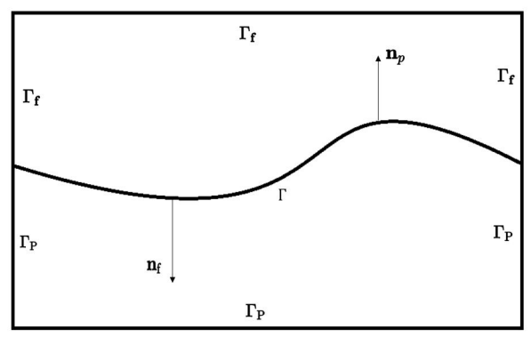
A global domain consisting of a fluid flow region
and a porous media flow region separated by an interface .
The fluid motion in the fluid region is governed by the Stokes equations
| (2.1) |
where
are the stress tensor and the deformation rate tensor, is the kinetic viscosity and is the external force.
We assume that the porous region possesses multiple scales. The fluid motion in the porous medium region is governed by
| (2.2) |
where denotes the hydraulic conductivity in , which is a positive symmetric tensor and includs multiscale information where is a small parameter and is a source term. The first equation is the saturated flow model and the second equation is the Darcy’s law. Here is the piezometric (hydraulic) head, where represents the dynamic pressure, the height from a reference level, the density and the gravitational constant, and is the flow velocity in the porous medium which is proportional to the gradient of , namely, the Darcy’s law.
Combining the two equations in (2.2), we get the equation for the piezometric head, which we will refer to simply as the Darcy equation:
| (2.3) |
Eqs. (2.1) and (2.3) are completed and coupled together by the following boundary conditions:
and the interface conditions on :
| (2.4) | |||
| (2.5) | |||
| (2.6) |
where is an orthonormal basis of the tangential space on and the gravitational acceleration and we assumed that in the following. is an experimentally determined parameter and represents the permeability, which has the following relation with the hydraulic conductivity, . The first interface condition (2.4) describes the mass conservation and the second equation (2.5) represents the balance of momentum. The third interface condtion (2.6) is called Beavers-Joseph-Saffman condition, which means the tangential components of the normal stress force is proportional to the tangential components of the fluid velocity[5].
Furthermore, we assume is symmetric, perodic, and uniformly elliptic. There exist two constants such that
Also, we assume
For simplicity, we consider 2D problems through the full text. We reserve for a domain (bounded and open set) with Lipschitz boundary and for spacial dimension . The Einstein summation convention is adopted, means summing repeated indexes from 1 to . The Sobolev spaces and are defined as usual (see e.g., [6]) and we abbreviate the norm Sobolev space as .
Later on we need to introduce some Hilbert spaces
| (2.7) |
The space , where or , is equipped with the usual -scalar product and -norm . The spaces and are equipped with the following norms:
Let us denote
Hence, we use the notational convention that and . They all belong to : for and , find such that and is the dual space of is the projection onto the local tangential plane that can be explicitly expressed as
| (2.8) |
where
| (2.9) | ||||
We know that there exists a positive constant such that the following Ladyzhenskaya-Babuš kaBrezzi (LBB) condition holds:
Remark 2.1.
For the purpose of later analysis, we recall some inequalities:
2.2 Finite element approximation
We give the finite element approximation of this model. For any given small parameter , we construct the regular triangulations and of and .
Let ,,and be finite element spaces such that the space pair satisfies the discrete LBB condition : there exists a constant ,independent of mesh ,such that
| (2.10) |
Here we choose MINI finite element pair for and multiscale finite element for . Define
We define Lagrange element space and consider a triangulation and base functions which consists of the globally continuous on and affine on each triangle functions which satisfy: ,where are the vertices of the coarse mesh ( the set of interior vertices of the coarse mesh) and is the Kronecker symbol. The multiscale finite element basis functions which take into account the multiscale of the coefficients. More precisely we compute , such that for any triangle ,
In practice, we do not have access to . We build , an approximation of on a finer embedded grid of mesh size , with FE. See Fig.2.
Therefore, we can get the multiscale finite element basis function and a simple observation tells that is locally support.

Then we can introduce
Therefore, the coupled finite element Galerkin approximation of reads:
Coupled Finite Element Scheme: find such that for any and
| (2.11) |
2.3 Homogenization theory and estimation results for the Darcy region
The Darcy region exhibits multiscale characteristics. In order to better elucidate our model, we introduce the model from [22]
| (2.12) |
For simplicity, we assume the source term belongs to , and the boundary term .
Then, we introduce the multiscale expansion technique in deriving homogenized equations. We look for in the form of asymptotic expansion
| (2.13) |
where the functions are periodic in with period 1 .
Here, we referenced some definitions and theorems from [22].
Definition 2.1.
A (vector/matrix value) function is called periodic, if and .
We need an interpolation operator. If the triangulation is regular, then there exist an interpolation operator , .
3 Multiscale finite Stokes-Darcy algorithm
In this section, we introduce the algorithm for the multiscale Stoke-Darcy equation. The algorithm is divided into two parts, namely the offline part and the online part. The offline part is used to compute the multiscale basis functions for the Darcy region. The online part utilizes the previously calculated multiscale basis functions and employs the Robin-Robin algorithm to obtain the solution of the equation.
3.1 Offline phase
In the offline phase, we solve the multiscale basis functions in parallel. This approach is adopted to enhance the efficiency of basis function generation.
-
•
The grid is partitioned to obtain the required coarse mesh .
-
•
For every , we build and parallelly solve in on with the standard basis function and store . See Fig.4.

Figure 3: -
•
Compute and store and with stifness matrix and the generic RHS.
-
•
Output: Assemble and store the stiffness matrix associted with the new basis

3.2 Online phase
In the online phase, we employ the Robin-Robin Stokes-Darcy algorithm. In this process, we utilize the multiscale basis functions generated in the offline stage. This algorithm is a decoupled algorithm, and here are the main steps:
-
•
Given the initial condtion , ,,.
-
•
For , independently solve the Stokes and Darcy systems with Robin boundary conditions. More precisely, find such that for all and it is
-
•
Find such that for all it is
-
•
Update and
-
•
Compute
-
•
If , then .
-
•
Output: get the soultion .
The offline phase involves a parallel method for generating multiscale basis functions. In the online phase, a Robin-Robin online Stokes-Darcy method is employed to obtain the solution. The algorithm offers advantages such as parallel construction of basis functions, which enhances reusability, and ensures high computational accuracy and efficiency. Additionally, the method is easily implementable for generalization and maintenance.
4 Error estimates
In this section, we analyze the error estimate of the above coupled multiscale finite element scheme (2.11). For later analysis, We define the following orthogonal projection from onto and from onto as: for any given and , find and such that
| (4.1) | ||||
For this projection and the projection from onto in the previous section, we make the following assumption: for any given and , there holds
| (4.2) |
Suppose the weak solution of the mixed Stokes/Darcy problem is local -regular, that is and
Theorem 4.1 ( norm).
Assume that is periodic, uniformly elliptic and symmtric. Let be a bounded Lipschitz domain in , and let and be the solutions of Problems (2.8) and (2.11), respectively.
| (4.3) | ||||
where depends on .
If we denote
Proof.
Recall the weak formulation and its finite element scheme
| (4.4) | ||||
where
| (4.5) | ||||
Then
| (4.9) | ||||
and we can get
| (4.10) | ||||
For ➀ :
| (4.11) | ||||
Then, we estimate the three terms on the right hand side of the above inequality.
For ➁ :
| (4.12) | ||||
For ➂ :
| (4.13) | ||||
For ➃ :
| (4.14) | ||||
Combining the above bounds and using (4.2) and Theorem 2.3, it yields
| (4.15) | ||||
Then, it is easily get the final result (4.3).
∎
Remark 4.1.
Given that , and are bounded, the norm can be controlled by .
Let us introduce the formal adjoint problem ([15]): find such that
| (4.16) |
where .
| (4.17) |
We assume that has the regularity estimate:
| (4.18) |
and
| (4.19) |
where and is the asymptotic expansion of .
Theorem 4.2 (L2 norm).
Assume that is periodic, uniformly ellpitic and symmtric. Let be a bounded Lipschitz domain in , and let and be the solutions of Problems (2.8) and (2.11), respectively.
| (4.20) | ||||
where depends on .
Remark 4.2.
Given that , and are bounded, the norm can be controlled by .
5 Numerical experiments
In this section, we study the accuracy of the multiscale method through numerical computations. The model problem is solved using the multiscale method with base functions defined by linear condition (Msfem). Since it is very diffcult to construct a test problem with exact solution and suffcient generality, we use resolved numerical solutions in place of exact solutions. The numerical results are compared with the theoretical analysis. Additionally, we present a numerical example illustrating the method’s application to more complex problems involving separable scales, nonseparable scales and high-contrast case.
5.1 Implementation
We outline the implementation here and define some notation to be frequently used below. For convenience, we assume that the multiscale Darcy region is situated on the unit square. Let be the number of elements in the and directions. The size of mesh is thus . To compute the base functions, each element is discretized into subcell elements with size . Triangular elements are used in all numerical tests.
In the offline phase, we utilize P1 elements to compute basis functions within each element. During this process, the Message Passing Interface(MPI) is employed to enhance efficiency, and the stiffness matrix and right-hand side are stored for subsequent online computations.
Because it is very difficult to construct a genuine steady Stokes-Darcy model with an exact solution, reference solutions are used as the exact solutions for the test problems. In all numerical examples below, the resolved solutions are obtained using standard FEM. We use the numerical computation libraries MUMPS and PETSc within FreeFEM++ to calculate the reference solution. Due to the multiscale nature of the permeability in our Darcy region, we employ a finer mesh within the Darcy region when computing the reference solution. We have computed a reference solution of this numerical example using Talor-Hood finite element and P2 element with a mesh of size (in Darcy region), (in Stokes region). The purpose of computing the reference solution is to obtain the error. To enhance computational speed, we utilize a domain decomposition parallel approach for computing the reference solution. We define the reference solution .
To facilitate the comparison among different schemes, we use the following shorthands: FEM-FEM stands for MINI elements in the Stokes region and P1 elements in the Darcy region and FEM-MsFEM stands for MINI elements in the Stokes region and multiscale basis function in the Darcy region. We define the numerical solution .
5.2 Numerical result
We define some norms to demonstrate the error.
5.2.1 Example 1
In this example, we we consider nonseparable scales and solve (2.3) with
where is a parameter controlling the magnitude of the oscillation. We take in this example. The right hand side function is zero On , we impose and on the , , . We set all physical parameters equal to 1. The Robin-Robin coefficients are set to .

The result of FEM-MsFEM error with varying but fixed and are shown in Table 1. When observing the errors in the Darcy part, we first fix the small parameter and gradually refine the grid. As decreases and , we can observe that the convergence order of the error for degrades from around to around . This effectively validates the term O() to O() in the error analysis. Additionally, the convergence order of the error degrades from to , providing a good validation of the term O() to O() in the error analysis. Furthermore, when observing the errors in the Stokes part, we use standard MINI elements in the Stokes region. However, it can be seen that the error in Stokes does not initially reach the optimal order of 2, and with the gradual decrease in grid size , the convergence order of the Stokes error also shows a decreasing trend. The reason for this decrease is influenced by the Darcy region, as the Darcy region also experiences a reduction in order at this point in time. Next, when observing the order of the velocity , it can be noted that the order does not initially reach the optimal order, but with a decrease in , the error order remains almost constant.
The result of FEM-FEM error with varying but fixed are shown in Table 2. When observing errors in the Darcy part, we first fix the small parameter . As decreases and , we can observe that the convergence orders of the error and error for pressure become unstable. Comparing with Table 1, it is noticeable that for , the error accuracy of FEM-MsFEM is higher than that of FEM-FEM. For instance, when , the accuracy of in the FEM-MsFEM algorithm can reach , whereas FEM-FEM can only achieve . When observing errors in the Stokes part, it can be noted that FEM-FEM does not reach the optimal order, and with the decrease in grid size , the convergence order of the Stokes error also shows a decreasing trend. The order of does not initially reach the optimal order, but with a decrease in , the error order remains almost constant. This result is consistent with the situation in FEM-MsFEM and is influenced by the Darcy region.
FEM-MsFEM error at , . are shown in Table 3. Our main goal is to observe errors in FEM-MsFEM when fixing , where . In the Darcy part, as gradually decreases, it can be observed that the and errors remain almost constant. This validates the importance of O() in the error and O() in the error. In the Stokes region, the convergence orders of and errors fail to reach the optimal order, and there is no significant change in the orders.
| Order | Order | Order | Order | |||||
|---|---|---|---|---|---|---|---|---|
| 1/4 | 6.07E-02 | 1.67E+00 | 8.99E-04 | 1.67E-02 | ||||
| 1/8 | 1.80E-02 | 1.76 | 9.44E-01 | 0.82 | 1.97E-04 | 2.19 | 7.56E-03 | 1.14 |
| 1/16 | 4.79E-03 | 1.91 | 5.07E-01 | 0.90 | 8.43E-05 | 1.23 | 4.82E-03 | 0.65 |
| 1/32 | 1.27E-03 | 1.92 | 2.69E-01 | 0.92 | 1.75E-04 | -1.05 | 5.05E-03 | -0.07 |
| 1/64 | 3.43E-04 | 1.89 | 1.41E-01 | 0.93 | 3.25E-04 | -0.89 | 6.82E-03 | -0.44 |
| 1/128 | 1.22E-04 | 1.49 | 7.41E-02 | 0.93 | 5.56E-04 | -0.78 | 9.47E-03 | -0.47 |
| 1/256 | 5.79E-05 | 1.07 | 3.85E-02 | 0.95 | 3.79E-04 | 0.55 | 7.85E-03 | 0.27 |
| Order | Order | Order | Order | |||||
|---|---|---|---|---|---|---|---|---|
| 1/4 | 6.07E-02 | 1.67E+00 | 5.31E-04 | 1.44E-02 | ||||
| 1/8 | 1.80E-02 | 1.76 | 9.44E-01 | 0.82 | 9.33E-04 | -0.81 | 1.34E-02 | 0.10 |
| 1/16 | 4.81E-03 | 1.90 | 5.07E-01 | 0.90 | 8.61E-04 | 0.12 | 1.26E-02 | 0.09 |
| 1/32 | 1.28E-03 | 1.91 | 2.69E-01 | 0.92 | 9.03E-04 | -0.07 | 1.27E-02 | -0.01 |
| 1/64 | 3.62E-04 | 1.83 | 1.41E-01 | 0.93 | 7.89E-04 | 0.19 | 1.19E-02 | 0.09 |
| 1/128 | 1.55E-04 | 1.22 | 7.41E-02 | 0.93 | 8.76E-04 | -0.15 | 1.23E-02 | -0.04 |
| 1/256 | 7.20E-05 | 1.11 | 3.85E-02 | 0.95 | 4.81E-04 | 0.86 | 8.73E-03 | 0.49 |
| Order | Order | Order | Order | ||||||
|---|---|---|---|---|---|---|---|---|---|
| 1/16 | 0.02 | 4.80E-03 | 5.07E-01 | 3.05E-04 | 6.89E-03 | ||||
| 1/32 | 0.01 | 1.27E-03 | 1.92 | 2.69E-01 | 0.92 | 2.88E-04 | 0.08 | 5.99E-03 | 0.20 |
| 1/64 | 0.005 | 3.38E-04 | 1.91 | 1.41E-01 | 0.93 | 2.80E-04 | 0.04 | 5.76E-03 | 0.06 |
| 1/128 | 0.0025 | 9.71E-05 | 1.80 | 7.41E-02 | 0.93 | 2.71E-04 | 0.05 | 5.63E-03 | 0.03 |
5.2.2 Example 2
In this example, we consider nonseparable scales and solve (2.3) with

where is a parameter controlling the magnitude of the oscillation. We take in this example. The right hand side function is zero
On , we impose and on the , , . We set all physical parameters equal to 1. The Robin-Robin coefficients are set to .
The result of FEM-MsFEM error with varying but fixed and are shown in Table 4. When examining errors in the Darcy part, we initially set a fixed small parameter and progressively refine the grid. As decreases, with , we observe a degradation in the convergence order of the error for from around to approximately . This observation effectively confirms the presence of terms O() to O() in the error analysis. Additionally, the convergence order of the error decreases from to , providing robust validation for terms O() to O() in the error analysis. Moreover, when evaluating errors in the Stokes part, standard MINI elements are employed in the Stokes region. However, it is evident that the error in Stokes does not initially attain the optimal order of 2. As the grid size gradually decreases, the convergence order of the Stokes error exhibits a declining trend. This decline is attributed to the influence of the Darcy region. Subsequently, when inspecting the order of the velocity , it is observed that the order does not initially reach the optimal level, yet with a decrease in , the error order remains relatively constant.
The result of FEM-FEM error with varying but fixed in Table 5. When observing errors in the Darcy part, we first fix the small parameter . As decreases and , we can observe that the convergence orders of the error and error for pressure become unstable. Comparing with Table 4, it is noticeable that for , the error accuracy of FEM-MsFEM is higher than that of FEM-FEM. For instance, when , the accuracy of in the FEM-MsFEM algorithm can reach , whereas FEM-FEM can only achieve . When observing errors in the Stokes part, it can be noted that FEM-FEM does not reach the optimal order, and with the decrease in grid size , the convergence order of the Stokes error also shows a decreasing trend. The order of does not initially reach the optimal order, but with a decrease in , the error order remains almost constant. This result is consistent with the situation in FEM-MsFEM and is influenced by the Darcy region.
FEM-MsFEM error at , . are shown in Table 6. Our main goal is to observe errors in FEM-MsFEM when fixing , where . In the Darcy part, as gradually decreases, it can be observed that the and errors remain almost constant. This validates the importance of O() in the error and O() in the error. In the Stokes region, the convergence orders of and errors fail to reach the optimal order, and there is no significant change in the orders.
| Order | Order | Order | Order | |||||
|---|---|---|---|---|---|---|---|---|
| 1/4 | 6.07E-02 | 1.67E+00 | 2.00E-03 | 3.12E-02 | ||||
| 1/8 | 1.80E-02 | 1.76 | 9.44E-01 | 0.82 | 5.06E-04 | 1.98 | 1.36E-02 | 1.20 |
| 1/16 | 4.79E-03 | 1.91 | 5.07E-01 | 0.90 | 8.65E-05 | 2.55 | 6.93E-03 | 0.97 |
| 1/32 | 1.26E-03 | 1.92 | 2.69E-01 | 0.92 | 6.31E-05 | 0.45 | 5.08E-03 | 0.45 |
| 1/64 | 3.34E-04 | 1.92 | 1.41E-01 | 0.93 | 1.23E-04 | -0.96 | 5.89E-03 | -0.21 |
| 1/128 | 9.44E-05 | 1.82 | 7.41E-02 | 0.93 | 2.28E-04 | -0.90 | 7.94E-03 | -0.43 |
| 1/256 | 3.28E-05 | 1.53 | 3.85E-02 | 0.95 | 1.70E-04 | 0.43 | 6.75E-03 | 0.23 |
| Order | Order | Order | Order | |||||
|---|---|---|---|---|---|---|---|---|
| 1/4 | 6.07E-02 | 1.67E+00 | 1.68E-03 | 2.91E-02 | ||||
| 1/8 | 1.80E-02 | 1.76 | 9.44E-01 | 0.82 | 4.96E-04 | 1.76 | 1.53E-02 | 0.93 |
| 1/16 | 4.80E-03 | 1.91 | 5.07E-01 | 0.90 | 3.30E-04 | 0.59 | 1.17E-02 | 0.39 |
| 1/32 | 1.27E-03 | 1.92 | 2.69E-01 | 0.92 | 4.21E-04 | -0.35 | 1.07E-02 | 0.13 |
| 1/64 | 3.37E-04 | 1.92 | 1.41E-01 | 0.93 | 2.68E-04 | 0.65 | 9.88E-03 | 0.11 |
| 1/128 | 1.03E-04 | 1.70 | 7.41E-02 | 0.93 | 3.69E-04 | -0.46 | 1.00E-02 | -0.02 |
| 1/256 | 3.73E-05 | 1.47 | 3.85E-02 | 0.95 | 2.11E-04 | 0.81 | 7.47E-03 | 0.42 |
| Order | Order | Order | Order | ||||||
|---|---|---|---|---|---|---|---|---|---|
| 1/16 | 0.02 | 4.79E-03 | 5.07E-01 | 1.16E-04 | 8.05E-03 | ||||
| 1/32 | 0.01 | 1.27E-03 | 1.92 | 2.69E-01 | 0.92 | 9.57E-05 | 0.28 | 5.76E-03 | 0.48 |
| 1/64 | 0.005 | 3.33E-04 | 1.92 | 1.41E-01 | 0.93 | 9.42E-05 | 0.02 | 5.13E-03 | 0.17 |
| 1/128 | 0.0025 | 8.87E-05 | 1.91 | 7.41E-02 | 0.93 | 9.07E-05 | 0.06 | 4.90E-03 | 0.07 |
References
- [1] Assyr Abdulle and Ondrej Budác. An adaptive finite element heterogeneous multiscale method for stokes flow in porous media. Multiscale Modeling & Simulation, 13(1):256–290, 2015.
- [2] Ilona Ambartsumyan, Eldar Khattatov, ChangQing Wang, and Ivan Yotov. Stochastic multiscale flux basis for stokes-darcy flows. Journal of Computational Physics, 401:109011, 2020.
- [3] Rodolfo Araya, Christopher Harder, Diego Paredes, and Frédéric Valentin. Multiscale hybrid-mixed method. SIAM Journal on Numerical Analysis, 51(6):3505–3531, 2013.
- [4] Todd Arbogast, Gergina Pencheva, Mary F. Wheeler, and Ivan Yotov. A multiscale mortar mixed finite element method. Multiscale Modeling & Simulation, 6(1):319–346 (electronic), 2007.
- [5] Gordon S Beavers and Daniel D Joseph. Boundary conditions at a naturally permeable wall. Journal of fluid mechanics, 30(1):197–207, 1967.
- [6] Susanne C Brenner. The mathematical theory of finite element methods. Springer, 2008.
- [7] Zhiming Chen and Thomas Y. Hou. A mixed multiscale finite element method for elliptic problems with oscillating coefficients. Mathematics of Computation, 72(242):541–576, 2003.
- [8] Eric T. Chung, Yalchin Efendiev, and Chak Shing Lee. Mixed generalized multiscale finite element methods and applications. Multiscale Modeling & Simulation, 13(1):338–366, 2015.
- [9] Marco Discacciati, Edie Miglio, and Alfio Quarteroni. Mathematical and numerical models for coupling surface and groundwater flows. Applied Numerical Mathematics, 43(1-2):57–74, 2002.
- [10] Y. Efendiev, V. Ginting, T. Hou, and R. Ewing. Accurate multiscale finite element methods for two-phase flow simulations. Journal of Computational Physics, 220(1):155–174, 2006.
- [11] Yalchin Efendiev, Juan Galvis, and Thomas Y. Hou. Generalized multiscale finite element methods (GMsFEM). Journal of Computational Physics, 251:116–135, 2013.
- [12] Vivette Girault, Danail Vassilev, and Ivan Yotov. Mortar multiscale finite element methods for stokes–darcy flows. Numerische Mathematik, 127(1):93–165, 2014.
- [13] Hadi Hajibeygi and Patrick Jenny. Multiscale finite-volume method for parabolic problems arising from compressible multiphase flow in porous media. Journal of Computational Physics, 228(14):5129–5147, 2009.
- [14] Thomas Y. Hou and Xiao-Hui Wu. A multiscale finite element method for elliptic problems in composite materials and porous media. Journal of computational physics, 134(1):169–189, 1997.
- [15] Yanren Hou and Yi Qin. On the solution of coupled stokes/darcy model with beavers–joseph interface condition. Computers & Mathematics with Applications, 77(1):50–65, 2019.
- [16] T. Hughes, G. Feijoo, L. Mazzei, and J. Quincy. The variational multiscale method - a paradigm for computational mechanics. Computer Methods in Applied Mechanics and Engineering, 166:3–24, 1998.
- [17] Patrick Jenny, SH Lee, and Hamdi A Tchelepi. Multi-scale finite-volume method for elliptic problems in subsurface flow simulation. Journal of computational physics, 187(1):47–67, 2003.
- [18] William J Layton, Friedhelm Schieweck, and Ivan Yotov. Coupling fluid flow with porous media flow. SIAM Journal on Numerical Analysis, 40(6):2195–2218, 2002.
- [19] Axel Målqvist and Daniel Peterseim. Localization of elliptic multiscale problems. Mathematics of Computation, 83(290):2583–2603, 2014.
- [20] E Weinan, Bjorn Engquist, Xiantao Li, Weiqing Ren, and Eric Vanden-Eijnden. Heterogeneous multiscale method: A review. Communications in Computational Physics, 2:367–450, 2007.
- [21] Ulrich Wilbrandt. Stokes–Darcy Equations: Analytic and Numerical Analysis. Springer, 2019.
- [22] Changqing Ye, Hao Dong, and Junzhi Cui. Convergence rate of multiscale finite element method for various boundary problems. Journal of Computational and Applied Mathematics, 374:112754, 2020.
- [23] Na Zhang, Jun Yao, Zhaoqin Huang, and Yueying Wang. Accurate multiscale finite element method for numerical simulation of two-phase flow in fractured media using discrete-fracture model. Journal of Computational Physics, 242:420–438, 2013.
- [24] Na Zhang, Jun Yao, Shifeng Xue, and Zhaoqin Huang. Multiscale mixed finite element, discrete fracture–vug model for fluid flow in fractured vuggy porous media. International Journal of Heat and Mass Transfer, 96:396–405, 2016.