Multiple states in turbulent large-aspect ratio thermal convection:
What determines the number of convection rolls?

For laminar flows, flow transitions can often be calculated from linear stability analysis. Such an analysis not only gives the critical value of the control parameter at which the instability sets in, but also the wavelength of the emerging structure. Famous classical examples for linearly unstable wall-bounded flows are the onset of convection rolls in Rayleigh-Bénard convection or the onset of Taylor rolls in Taylor-Couette flow dra81 . In both cases, the rolls of the most unstable mode have a certain wavelength which follows from the linear stability analysis. With increasing flow driving strength, more and more modes become unstable, and in the fully turbulent case the base flow is unstable to basically any perturbation.

What then sets the size of the flow structures in such fully turbulent wall-bounded flow? Recent findings have suggested that wall-bounded turbulent flows can take different statistically stationary turbulent states, with different length scale of the flow structures and with different transport properties, even for the very same values of the control parameters. Examples for the coexistence of such multiple turbulent states include turbulent (rotating) Rayleigh-Bénard convection xi08 ; poe11 ; poe12 ; weiss2013 ; wang2018 ; xie2018 ; favier2019 , Taylor-Couette turbulence hui14 ; veen2016 ; ost16 , von Karman flow rav04 ; rav08 ; cor10 ; faranda2017 , rotating spherical Couette flow zim11 , Couette flow with span-wise rotation xia2018 , but also geophysical flows bouchet2009random ; bouchet2012statistical such as in ocean circulation broecker1985 ; schmeits2001 ; ganopolski2002 , in the liquid metal core of Earth glatzmaiers1995 ; li2002 ; olson2010 ; sheyko2016magnetic , or in the atmosphere weeks1997 ; bouchet2019rare .

The occurrence of multiple states in fully turbulent flows can be considered unexpected since, according to Kolmogorov kol41b , for strong enough turbulence, the fluctuations should become so strong that the whole highly dimensional phase-space is explored. Of course, one could argue that in the above given cases and examples, the turbulence driving has not yet been strong enough to reach that state and that the occurrence of multiple turbulent states in wall-bounded turbulence may be a finite size effect, but in any case even then it remains open what sets the range of allowed sizes of the flow structures in such turbulent flows.

To illuminate this question, as a model system we picked two-dimensional (2D) Rayleigh–Bénard (RB) turbulence, the flow in a closed container heated from below and cooled from above ahl09 ; loh10 ; chi12 . The control parameters are the Rayleigh number $Ra$, which is the dimensionless temperature difference between the plates, the Prandtl number $Pr$, which is the ratio between kinematic viscosity ($\nu$) and thermal diffusivity ($\kappa$), and the aspect ratio $\Gamma=W/H$, i.e., the ratio between horizontal ($W$) and vertical ($H$) extension of the system. The response parameters are the Nusselt number $Nu={QH}/{(k\Delta})$ and the Reynolds number $Re={UH}/{\nu}$, which indicate the dimensionless heat transport and flow strength in the system. Here $Q$ is the heat flux crossing the system, $k$ the thermal conductivity, $\Delta$ the temperature difference at the plates, and $U=\sqrt{\langle{\bf u}^{2}\rangle_{V,t}}$ the time and volume-averaged velocity.

The flow dynamics is given by the Boussinesq approximation of the Navier-Stokes and the advection-diffusion equation, with the corresponding boundary conditions (BCs) for the temperature and velocity fields. For the latter at the plates we will first apply no-slip BCs, but later also examine free-slip BCs – a difference which will turn out to be major for the range of allowed states. Periodic BCs are used in the horizontal direction.

We are very much aware of the differences between 2D and 3D RB flow poe13 , but in particular for large $Pr\geq 1$ there are extremely close similarities between 2D and 3D RB flows, and we wanted to pick a model system for which (i) we can reasonably explore the considerable parameter space for a large enough number of initial flow conditions and (ii) we have the chance to obtain exact analytical results for the range of allowed flow structures.

The parameter range we will explore is for large Prandtl numbers in the range $1\leq Pr\leq 100$, for Rayleigh numbers in the range $10^{7}\leq Ra\leq 10^{10}$ and for large $\Gamma$ up to $\Gamma=32$. Note that in 2D RB, multiple coexisting turbulent states had been found before for $Ra=10^{7}$, $Pr=0.7$ and $\Gamma\approx 0.64$ (i.e., in an extremely limited range of the parameter space) poe11 , but not for such large $\Gamma$ and $Ra$ as we explore here, as the range of chosen initial flow conditions was not large enough poe12 , and clearly not as general and omnipresent as we will find here.

The direct numerical simulations were done with an advanced finite difference code (AFiD poe15cf ) with the criteria for the grid resolution, as found to be required in ref. shi10 . The code has extensively been tested and benchmarked against other codes kooij2018 and applied in 2D RB even up to very large $Ra=4.64\times 10^{14}$ zhu18b ; zhu2019reply . More simulation details for all explored cases can be found in the supplementary material. In order to trigger the possible convection roll state, we use different initial roll states generated by a Fourier basis: $u(x,z)={\rm sin}(n^{(i)}\pi x/\Gamma){\rm cos}(\pi z)$, $w(x,z)=-{\rm cos}(n^{(i)}\pi x/\Gamma){\rm sin}(\pi z)$, where $n^{(i)}$ indicates the initial number of rolls in the horizontal direction. The initial temperature has a linear profile with random perturbations.

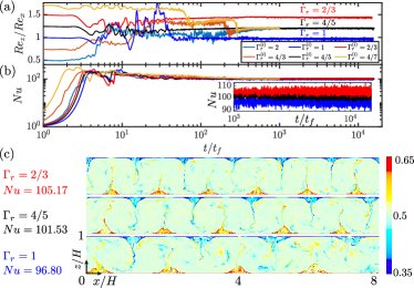
In Fig. 1(a) and  1(b) we show the temporal evolution of some flow characteristics for six different initial flow conditions for the case of $Ra=10^{10}$, $Pr=10$, and $\Gamma=8$. We vary the initial number $n^{(i)}$ of rolls from $n^{(i)}=4$ to $n^{(i)}=14$, implying aspect ratios of the initial rolls from $\Gamma_{r}^{(i)}=\Gamma/n^{(i)}=2$ to $\Gamma_{r}^{(i)}=4/7$. As flow characteristics we picked the Reynolds number ratio $Re_{z}/Re_{x}$ and the Nusselt number $Nu$. Here $Re_{z}=\sqrt{\langle w^{2}\rangle_{V}}H/\nu$ is the volume averaged vertical Reynolds number and $Re_{x}=\sqrt{\langle u^{2}\rangle_{V}}H/\nu$ the horizontal one, where $w(t)$ and $u(t)$ are the respective velocities. As one can see in Fig. 1(a, b), depending on the six initial conditions, over the very long time of more than $10^{4}$ free-fall time units, the system evolves to either of three different final turbulent states, all with different Reynolds number ratio $Re_{z}/Re_{x}$ and Nusselt number $Nu$. The smaller the final mean aspect ratio $\Gamma_{r}$ of the rolls, the larger the Reynolds number ratio $Re_{z}/Re_{x}$ and $Nu$, due to more plume-ejecting regions which have strong vertical motion.

The time evolution of some of the six different initial states ($n^{(i)}=6,14$) analyzed in Fig. 1(a, b) can be seen in the supplementary movies, displaying roll merging and splitting events. The states with large initial rolls (corresponding to $n^{(i)}=4$, 6) break up quickly, while those with small initial rolls ($n^{(i)}=14$) first undergo a transition into an unstable twelve-roll state (with smaller $Re_{z}/Re_{x}$ than the stable one) as seen in Fig. 1(a), followed by merging events of two neighboring convection rolls. Though both, the Reynolds number ratio and the Nusselt number, keep on fluctuating in time, reflecting the turbulent nature of the states, the three final statistically stable turbulent states are clearly distinguished. We characterize them by the final aspect ratio of their rolls, namely $\Gamma_{r}=1$, $\Gamma_{r}=4/5$, and $\Gamma_{r}=2/3$, corresponding to $n=\Gamma/\Gamma_{r}=8$, 10, and 12 rolls, respectively. Snapshots of these states and their corresponding Nusselt numbers are shown in Fig. 1(c). As one can see, the larger the number of rolls, the better the (heat) transport properties of the system, a characteristics which was found in Taylor-Couette flow before hui14 and which can intuitively be understood, due to the larger number of emitted plumes at the interfaces between the rolls.

Consequently, when the cell aspect ratio $\Gamma$ is stretched, the stretching of the mean aspect ratio $\Gamma_{r}=\Gamma/n$ of the corresponding individual rolls is accompanied with a decrease of the corresponding Nusselt number, as seen in Fig. 2(a) and 2(b). Though this behavior has been seen before poe12 , in Fig. 2(a) and 2(b) we clearly see the coexistence of the different turbulent states. The determining relevance of the final mean aspect ratio $\Gamma_{r}=\Gamma/n$ of the individual rolls for the Nusselt number $Nu$ and Reynolds number $Re$ in the statistically stationary case is nicely demonstrated in Fig. 2(c) and 2(d), where we show that the dependences $Nu(\Gamma_{r})$ and $Re(\Gamma_{r})$ are universal and irrespective of the individual values of $\Gamma$ or $n$.

Remarkably, not only the absolute value of the Nusselt number depends on $\Gamma_{r}$, but even the effective scaling behavior of $Nu$ with $Ra$, as can be seen in Fig. 3(a). The same holds for the Reynolds number, Fig. 3(b). In both cases the effective scaling exponent is larger for turbulent states with smaller mean aspect ratio $\Gamma_{r}$ of the rolls (see the values given in Fig 3(a,b)), i.e., when the system can accommodate a larger number $n=\Gamma/\Gamma_{r}$ of rolls, presumably reflecting the larger disorder and the larger number of emitted plumes for those states.

From Fig. 3(a,b) we also see that turbulent states with a too large aspect ratio $\Gamma_{r}$ of their rolls cease to exist with increasing $Ra$. Which turbulent states – as characterized by the mean aspect ratio $\Gamma_{r}$ of their rolls – are statistically stable for given $Ra$ and $Pr$ can be seen from the phase diagrams in Fig. 4. For fixed $Pr=10$, all statistically stable turbulent states in the no-slip case have an aspect ratio $\Gamma_{r}$ in the range $2/3\leq\Gamma_{r}\leq 4/3$, in the $Ra$-range analyzed in this paper. With increasing $Ra$, we see the range moving towards smaller values of $\Gamma_{r}$; e.g. with $1\leq\Gamma_{r}\leq 4/3$ for $Ra=10^{8}$ and $2/3\leq\Gamma_{r}\leq 1$ for $Ra=10^{10}$, see figure 4(a). For $Ra=10^{9}$, we find $2/3\leq\Gamma_{r}\leq 1$ for all $Pr$ analysed in this paper, see Fig. 4(b).

We now set out to mathematically understand the range of $\Gamma_{r}$ the system can take for given control parameters. First, we recall that the roll size is restricted by the elliptical instability of the flow landman1987 ; waleffe1990 ; kerswell2002 ; zwirner2020 . We therefore assume that the essence of the flow is a set of elliptical rolls, each of which can be described by a stream function $\Psi(x,z)=(\xi+\eta){z^{2}\over 2}+(\xi-\eta){x^{2}\over 2}$ with $\xi\geq\eta$. The aspect ratio of the rolls, $\Gamma_{r}$, is directly related to the strain $\eta$ and (half of) the vorticity $\xi$ through the relation $\Gamma_{r}=\sqrt{(\xi+\eta)/(\xi-\eta)}$, corresponding to $\eta/\xi=(\Gamma_{r}^{2}-1)/(\Gamma_{r}^{2}+1)$. Averaging $u^{2}$ and $w^{2}$ over the area $[-\Gamma_{r}H/2,\,\Gamma_{r}H/2]\times[-H/2,\,H/2]$, where $u(x,z)=\partial\Psi/\partial z$ and $w(x,z)=-\partial\Psi/\partial x$, we obtain $Re_{x}^{2}=\Gamma_{r}^{2}Re_{z}^{2}$, which is in agreement with the simulations, see supplementary material.

As shown in refs. landman1987 ; waleffe1990 , the growth rate $\sigma=\sigma(\eta/\xi)$ of the elliptical instability is $\sigma\approx 9\eta/16$ for small $\eta/\xi$ and achieves its maximum $\sigma_{\max}\approx 0.35\xi$ at $\eta/\xi\approx 0.8$. Fourier modes of the kinetic energy $E$ of the perturbations follow $\sigma E=dE/dt$ ($=\partial E/\partial t+{\bf u}\cdot\nabla E$) and their averages ($\overline{\cdot}$) in time and over the roll core $\sigma\overline{E}\lesssim(\sqrt{\overline{{\bf u}^{2}}}/H)\overline{E}$, implying that the growth rate of the instability is bounded by the mean velocity of the carrying flow, i.e.,

$$\sigma\lesssim(\nu/H^{2})Re.$$

(1)

We now make use of the exact global balance for the total enstrophy $\Omega^{2}$ and the mean kinetic energy dissipation rate $\epsilon_{u}$ shr90 , namely, $4\nu\xi^{2}=\nu\Omega^{2}=\epsilon_{u}=\nu^{3}H^{-4}(Nu-1)RaPr^{-2}$. With the definition

$$B\equiv{Re^{2}\,Pr^{2}Ra^{-1}(Nu-1)^{-1}}$$

(2)

(which can be seen as non-dimensionalized ratio between the kinetic energy and the energy dissipation rate) this leads to $\sigma_{\max}\approx 0.35\xi=0.175\nu H^{-2}Re/\sqrt{B}$, implying that relation (1) is fulfilled when $\sqrt{B}>0.175$ (i.e., when $B\gtrsim 0.03$). For smaller $B$, from Eq. (1) and the relation between the ratio $\eta/\xi$ and $\Gamma_{r}$, we obtain $Re\geq\frac{9}{16}\eta\frac{H^{2}}{\nu}=\frac{9}{32}(\Gamma_{r}^{2}-1)/(\Gamma_{r}^{2}+1)\sqrt{Ra(Nu-1)}/Pr$, which gives an estimate of the maximal size of the rolls as

$$\Gamma_{r}\leq\sqrt{9+32\sqrt{B}}/\sqrt{9-32\sqrt{B}}.$$

(3)

Figs. 5(a, b) show the $Ra$- and $Pr$-dependences of $B$, obtained numerically for the no-slip BCs, as well as their data fits (see supplementary material). As seen from the phase diagrams in Figs. 4(a, b), using these fits in Eq. (3) gives quite reasonable estimates for the maximal mean roll size of statistically stable turbulent states, see upper blue lines in Figs. 4(a, b).

We now come to the lower bound of the window of allowed $\Gamma_{r}$. First note that $\Gamma_{r}$ cannot be infinitesimally small, because, in order to form the rolls, the growth rate of the elliptical instability should be much larger than the viscous damping rate, i.e., $\sigma\gg\nu/H^{2}$. One can obtain a more accurate estimate when considering a rectangular region that frames a particular roll. Under the assumption that the velocity components achieve their maximum at the boundaries of this rectangle or vanish there, there exists a certain constant $c>2$ such that $c^{2}\overline{{\bf u}^{2}}\leq\Gamma_{r}^{2}H^{2}\overline{(\nabla{\bf u})^{2}}$. We call this relation the generalized Friedrichs inequality and derive it in the supplementary material. This inequality gives as estimate for the lower bound of $\Gamma_{r}$

$$\Gamma_{r}\geq c\sqrt{B},$$

(4)

which is plotted as lower blue lines in Fig. 4(a, b) for $c=9$. As can be seen, the theoretical slopes reflect the general tendency of the numerical results. Note however that at this point we cannot calculate the absolute value of the transition, i.e., the value of $c$. We also remark that in the case when the container is too slender to keep 2 rolls (with the size, according to (4)), i.e., when $\Gamma<2c\sqrt{B}$, the flow can take the form of a zonal flow only. Thus, in the no-slip case, the zonal flow configuration van2014effect ; goluskin2014 is possible, but only in small-aspect ratio containers.

Our approach also leads to reasonable estimates for the window of allowed statistically stable states in the free-slip case, which was numerically analyzed in ref. wang2020zonal : Taking the dependences $Nu(Ra,Pr)$ and $Re(Ra,Pr)$ for the various roll states from that work, with the definition (2) we obtain $B(Ra,Pr)$, see Figs. 5(c, d). The value of $B$ is always larger than 0.03. Therefore (as discussed above), in the free-slip case, the relation (1) is always fulfilled without any restriction on the maximal roll size. Thus, very large-$\Gamma_{r}$ states are possible, while particular state realizations depend on the initial conditions. Indeed, this is consistent with the numerical findings in ref. wang2020zonal , which are shown in Figs. 4(c, d). Note in particular that in ref. wang2020zonal an as large stable state as $\Gamma_{r}=64$ (for $\Gamma=128$, $Ra=10^{8}$, $Pr=10$) was found.

What about the lower bound for allowed $\Gamma_{r}$ in the free-slip case? In contrast to the upper bound, it does exist, and just as in the no-slip case, by arguments again based on the generalized Friedrich inequality (see supplementary material), we can find it. In Fig. 4(c, d) the result for the smallest $\Gamma_{r}$ is plotted. It is based on the estimate (4) and uses the fits from Fig. 5(c, d) for the smallest values of $B$ with $c=7$. Again, the theoretical slopes in the $\Gamma_{r}-Ra$ and $\Gamma_{r}-Pr$ phase diagrams reflect the general trend of the numerical results.

In conclusion, we have numerically shown the coexistence of multiple statistically stable states in turbulent RB convection with no-slip BCs, with different mean aspect ratios of their turbulent rolls and different transport properties, even scaling-wise. We then theoretically illuminated what principles determine the allowed window of the mean size of the turbulent convection rolls (and thus their absolute number), namely, the existence of the elliptical instability and viscous damping. These criteria also work for the free-slip case.

Even though a 2D model may seem somehow artificial, there are various cases in which the flow dynamics is mostly 2D, e.g. because of geometrical confinement, stratification or background rotation. Therefore our model in itself is relevant, but the main ideas of our approach can also be generalized to other wall-bounded turbulent flows, such as rotating Rayleigh-Bénard flow, Taylor-Couette flow, Couette flow with span-wise rotation, double diffusive convection, etc., and also to geophysical flows such as those mentioned in the introduction. They may also give guidance for turbulence flow control, in order to predict which turbulent states are feasible to be realizable.

Acknowledgements: We acknowledge the Deutsche Forschungsgemeinschaft (Priority Programme SPP 1881 “Turbulent Superstructures”). This work was partly carried out on the national e-infrastructure of SURFsara.

References

- (1) P. Drazin and W. H. Reid, Hydrodynamic stability (Cambridge University Press, Cambridge, 1981).
- (2) H.-D. Xi and K.-Q. Xia, Flow mode transitions in turbulent thermal convection, Phys. Fluids 20, 055104 (2008).
- (3) E. P. van der Poel, R. J. A. M. Stevens, and D. Lohse, Connecting flow structures and heat flux in turbulent Rayleigh-Bénard convection, Phys. Rev. E 84, 045303(R) (2011).
- (4) E. P. van der Poel, R. J. A. M. Stevens, and D. Lohse, Flow states in two-dimensional Rayleigh-Bénard convection as a function of aspect-ratio and Rayleigh number, Phys. Fluids 24, 085104 (2012).
- (5) S. Weiss and G. Ahlers, Effect of tilting on turbulent convection: cylindrical samples with aspect ratio , J. Fluid Mech. 715, 314 (2013).
- (6) Q. Wang, Z.-H. Wan, R. Yan, and D.-J. Sun, Multiple states and heat transfer in two-dimensional tilted convection with large aspect ratios, Phys. Rev. Fluids 3, 113503 (2018).
- (7) Y.-C. Xie, G.-Y. Ding, and K.-Q. Xia, Flow topology transition via global bifurcation in thermally driven turbulence, Phys. Rev. Lett. 120, 214501 (2018).
- (8) B. Favier, C. Guervilly, and E. Knobloch, Subcritical turbulent condensate in rapidly rotating Rayleigh–Bénard convection, J. Fluid Mech. 864, R1 (2019).
- (9) S. G. Huisman, R. C. A. van der Veen, C. Sun, and D. Lohse, Multiple states in highly turbulent Taylor-Couette flow, Nat. Commun. 5, 3820 (2014).
- (10) R. C. van der Veen, S. G. Huisman, O.-Y. Dung, H. L. Tang, C. Sun, D. Lohse, et al., Exploring the phase space of multiple states in highly turbulent Taylor-Couette flow, Phys. Rev. Fluids 1, 024401 (2016).
- (11) R. Ostilla-Mónico, D. Lohse, and R. Verzicco, Effect of roll number on the statistics of turbulent Taylor-Couette flow, Phys. Rev. Fluids 1, 054402 (2016).
- (12) F. Ravelet, L. Marié, A. Chiffaudel, and F. Daviaud, Multistability and memory effect in a highly turbulent flow: Experimental evidence for a global bifurcation, Phys. Rev. Lett. 93, 164501 (2004).
- (13) F. Ravelet, M. Berhanu, R. Monchaux, S. Aumaitre, A. Chiffaudel, F. Daviaud, B. Dubrulle, M. Bourgoin, P. Odier, N. Plihon, J. F. Pinton, R. Volk, S. Fauve, N. Mordant, and F. Petrelis, Chaotic dynamos generated by a turbulent flow of liquid sodium, Phys. Rev. Lett. 101, 074502 (2008).
- (14) P. Cortet, A. Chiffaudel, F. Daviaud, and B. Dubrulle, Experimental evidence of a phase transition in a closed turbulent flow, Phys. Rev. Lett. 105, 214501 (2010).
- (15) D. Faranda, Y. Sato, B. Saint-Michel, C. Wiertel, V. Padilla, B. Dubrulle, and F. Daviaud, Stochastic chaos in a turbulent swirling flow, Phys. Rev. Lett. 119, 014502 (2017).
- (16) D. S. Zimmerman, A. A. Triana, and D. P. Lathrop, Bi-stability in turbulent, rotating spherical Couette flow, Phys. Fluids 23, 065104 (2011).
- (17) Z. Xia, Y. Shi, Q. Cai, M. Wan, and S. Chen, Multiple states in turbulent plane Couette flow with spanwise rotation, J. Fluid Mech. 837, 477 (2018).
- (18) F. Bouchet and E. Simonnet, Random changes of flow topology in two-dimensional and geophysical turbulence, Phys. Rev. Lett. 102, 094504 (2009).
- (19) F. Bouchet and A. Venaille, Statistical mechanics of two-dimensional and geophysical flows, Physics reports 515, 227 (2012).
- (20) W. S. Broecker, D. M. Peteet, and D. Rind, Does the ocean–atmosphere system have more than one stable mode of operation?, Nature 315, 21 (1985).
- (21) M. J. Schmeits and H. A. Dijkstra, Bimodal behavior of the Kuroshio and the Gulf Stream, J. Phys. Oceanogr. 31, 3435 (2001).
- (22) A. Ganopolski and S. Rahmstorf, Abrupt glacial climate changes due to stochastic resonance, Phys. Rev. Lett. 88, 038501 (2002).
- (23) G. A. Glatzmaiers and P. H. Roberts, A three-dimensional self-consistent computer simulation of a geomagnetic field reversal, Nature 377, 203 (1995).
- (24) J. Li, T. Sato, and A. Kageyama, Repeated and sudden reversals of the dipole field generated by a spherical dynamo action, Science 295, 1887 (2002).
- (25) P. L. Olson, R. S. Coe, P. E. Driscoll, G. A. Glatzmaier, and P. H. Roberts, Geodynamo reversal frequency and heterogeneous core–mantle boundary heat flow, Phys. Earth and Planetary Interiors 180, 66 (2010).
- (26) A. Sheyko, C. C. Finlay, and A. Jackson, Magnetic reversals from planetary dynamo waves, Nature 539, 551 (2016).
- (27) E. R. Weeks, Y. Tian, J. Urbach, K. Ide, H. L. Swinney, and M. Ghil, Transitions between blocked and zonal flows in a rotating annulus with topography, Science 278, 1598 (1997).
- (28) F. Bouchet, J. Rolland, and E. Simonnet, Rare event algorithm links transitions in turbulent flows with activated nucleations, Phys. Rev. Lett. 122, 074502 (2019).
- (29) A. N. Kolmogorov, On degeneration (decay) of isotropic turbulence in incompressible viscous liquid, Dokl. Akad. Nauk SSSR 31, 538 (1941).
- (30) G. Ahlers, S. Grossmann, and D. Lohse, Heat transfer and large scale dynamics in turbulent Rayleigh-Bénard convection, Rev. Mod. Phys. 81, 503 (2009).
- (31) D. Lohse and K.-Q. Xia, Small-scale properties of turbulent Rayleigh-Bénard convection, Annu. Rev. Fluid Mech. 42, 335 (2010).
- (32) F. Chilla and J. Schumacher, New perspectives in turbulent Rayleigh-Bénard convection, Eur. Phys. J. E 35, 58 (2012).
- (33) E. P. van der Poel, R. J. A. M. Stevens, and D. Lohse, Comparison between two- and three-dimensional Rayleigh-Bénard convection, J. Fluid Mech. 736, 177 (2013).
- (34) E. P. van der Poel, R. Ostilla-Mónico, J. Donners, and R. Verzicco, A pencil distributed finite difference code for strongly turbulent wall–bounded flows, Computers & Fluids 116, 10 (2015).
- (35) O. Shishkina, R. J. A. M. Stevens, S. Grossmann, and D. Lohse, Boundary layer structure in turbulent thermal convection and its consequences for the required numerical resolution, New J. Phys. 12, 075022 (2010).
- (36) G. L. Kooij, M. A. Botchev, E. M. Frederix, B. J. Geurts, S. Horn, D. Lohse, E. P. van der Poel, O. Shishkina, R. J. A. M. Stevens, and R. Verzicco, Comparison of computational codes for direct numerical simulations of turbulent Rayleigh–Bénard convection, Computers & Fluids 166, 1 (2018).
- (37) X. Zhu, V. Mathai, R. J. A. M. Stevens, R. Verzicco, and D. Lohse, Transition to the Ultimate Regime in Two-Dimensional Rayleigh-Bénard Convection, Phys. Rev. Lett. 120, 144503 (2018).
- (38) X. Zhu, V. Mathai, R. J. A. M. Stevens, R. Verzicco, and D. Lohse, Reply to “Absence of evidence for the ultimate regime in two-dimensional Rayleigh-Bénard convection.”, Phys. Rev. Lett. 123, 259402 (2019).
- (39) M. Landman and P. Saffman, The three-dimensional instability of strained vortices in a viscous fluid, Phys. Fluids 30, 2339 (1987).
- (40) F. Waleffe, On the three-dimensional instability of strained vortices, Phys. Fluids A 2, 76 (1990).
- (41) R. R. Kerswell, Elliptical instability, Annu. Rev. Fluid Mech. 34, 83 (2002).
- (42) L. Zwirner, A. Tilgner, and O. Shishkina, Elliptical Instability and Multi-Roll Flow Modes of the Large-scale Circulation in Confined Turbulent Rayleigh-Bénard Convection, arXiv preprint arXiv:2002.06951 (2020).
- (43) B. I. Shraiman and E. D. Siggia, Heat transport in high-Rayleigh number convection, Phys. Rev. A 42, 3650 (1990).
- (44) E. P. van der Poel, R. Ostilla-Mónico, R. Verzicco, and D. Lohse, Effect of velocity boundary conditions on the heat transfer and flow topology in two-dimensional Rayleigh-Bénard convection, Phys. Rev. E .
- (45) D. Goluskin, H. Johnston, G. R. Flierl, and E. A. Spiegel, Convectively driven shear and decreased heat flux, J. Fluid Mech. 759, 360 (2014).
- (46) Q. Wang, K.-L. Chong, R. J. A. M. Stevens, R. Verzicco, and D. Lohse, From zonal flow to convection rolls in Rayleigh-Bénard convection with free-slip plates, arXiv:2005.02084 .