Multiple soliton solutions and similarity reduction of a (2+1)-dimensional variable-coefficient Korteweg–de Vries system
Abstract
In this paper, we study the novel nonlinear wave structures of a (2+1)-dimensional variable-coefficient Korteweg–de Vries (KdV) system by its analytic solutions. Its -soliton solution are obtained via Hirota’s bilinear method, and in particular, the hybrid solution of lump, breather and line soliton are derived by the long wave limit method. In addition to soliton solutions, similarity reduction, including similarity solutions (also known as group-invariant solutions) and non-autonomous third-order Painlevé equations, is achieved through symmetry analysis. The analytic results, together with illustrative wave interactions, show interesting physical features, that may shed some light on the study of other variable-coefficient nonlinear systems.
Keywords: (2+1)-dimensional variable-coefficient KdV system, Hirota’s bilinear method, soliton solution, symmetry, similarity solution.
1 Introduction
Nonlinear partial differential equations play a crucial role in modeling wave phenomena that arise in various fields, such as fluid mechanics, nonlinear optics, plasma physics, condensed matter physics, etc. Methods for constructing their analytical solutions, that can explicitly describe the dynamical behavior, have attracted much attention, among which there are the Hirota’s bilinear method [18, 21], Darboux transformation [16, 47], the inverse scattering transformation [2, 41], the multiple exp-function method [26], dressing method [29, 22], symmetry method [20, 33, 19, 6, 37], and so on. In the current paper, we will mainly be focused on soliton solutions by Hirota’s bilinear method and similarity solution by symmetry reduction.
Hirota’s bilinear method has been investigated by many scholars (see, e.g., [13, 38]). For integrable nonlinear evolution equations, Hirota’s bilinear method can be used to construct -soliton solutions applying the superposition of solutions, and has been extended to obtain breather, lump and their interaction solutions [24], higher-order localized wave [14], rational and semi-rational solution [17]. It was also employed for searching the localized waves of nonlocal evolution equations [48, 49] and variable-coefficient evolution equations [23, 36, 45].
On the other hand, continuous symmetries have also been widely applied to the analysis of differential equations (see, e.g., [7, 34, 35]). They can lead to exact solutions or reductions of differential equations [33, 6], and are closely relevant to their integrability (see, e.g., [30]). In recent years, symmetry analysis of variable-coefficient evolution equations has attracted much attention. For instance, in [32, 31], Mohamed and co-authors investigated lump soliton, solitary waves and exponential solutions of the (3+1) dimensional variable-coefficients Kudryashov–Sinelshchikov equation and the (2+1)-dimensional variable-coefficient Bogoyavlensky–Konopelchenko equation by similarity reduction using their symmetries. In [44], a variable-coefficient Davey–Stewartson system was studied, where the optimal system of symmetries was obtained with adjoint representation. Variable-coefficient Davey–Stewartson system that admits the Kac-Moody-Virasoro symmetry was proposed in [15]. In [46], nonlocal symmetries of the coupled variable-coefficient Newell–Whitehead system were used to calculate its group-invariant solutions. However, few studies have been conduced on the dynamics of higher-order localized waves. In the current paper, we focus on nonlinear wave structures of the following (2+1)-dimensional variable-coefficient Korteweg–de Vries (KdV) system
| (1.1) |
and particularly its integrable variant with both and constant functions, using both Hirota’s bilinear method and symmetry analysis. Here, , are the dependent variables and , and are the independent variables. The notations , and so forth are adopted in the current paper. The functions , and are known but arbitrary functions of which are assumed to be smooth enough; when , the system (1.1) reduces to the constant-coefficient (2+1)-dimensional KdV system [42, 25], derived by Boiti et al. using the weak Lax pair [11]. Furthermore, the system (1.1) reduces to the (1+1)-dimensional KdV equation by setting and .
In Section 2, integrability condition of (1.1) is analyzed by Painlevé analysis and in what follows we will be focused on its integrable version with constant coefficients and . In Section 3, -soliton solutions and hybrid interaction of line solitons, and breather and lump solitons are obtained through Hirota’s bilinear method, while in Section 4, we invoke the symmetry method to derive Lie point symmetries and obtain the corresponding similarity solutions. In particular, a PDE (see Eq. (4.16) or system (4.14) in the potential form below) passing the Painlevé test is derived by symmetry reduction, that reads
| (1.2) |
where are the independent variables and is the dependent variable, and is an arbitrary function. Further symmetry reduction shows that it can be reduced to non-autonomous third-order Painlevé equations, which are in the form of Chazy’s classification of third-order ODEs by Painlevé analysis but not included in Chazy’s 13 classes. The final Section 5 is dedicated to conclusion.
2 Painlevé analysis of the variable-coefficient KdV system
In this section, we study integrability condition of the (2+1)-dimensional variable-coefficient KdV system (1.1) through Painlevé analysis (see, e.g., [40, 43]). Let and , and the system (1.1) becomes
| (2.1) |
that is assumed to admit a solution as a Laurent expansion about a singular manifold as follows
| (2.2) |
Here, is determined by a leading-term analysis and balancing the dominant terms and . Straightforward calculation gives and
| (2.3) |
Substituting back to Eq. (2.2) and balancing the most singular term again, we obtain
| (2.4) |
Combining Eqs. (2.3) and (2.4), is arbitrary when and , which are the resonant points. Substitution of (2.2) into Eq. (2.1) then amounts to the recursion relations for the , which take the form of coupled partial differential equations. Finally, we observe that explicit expressions for , and and compatibility condition to ensure integrability requires , to be non-zero constants, but remains to be an arbitrary function of . Consequently, , and are arbitrary functions.
To summarize up, we conclude that the following special (2+1)-dimensional time-dependent variable-coefficient KdV system
| (2.5) |
is integrable as passes the Painlevé test, where and are constants. In the rest of the paper, we will be focused on studies of analytic solutions of the integrable system (2.5).
3 Bilinear representation and -solitons
The integrable (2+1)-dimensional time-dependent variable-coefficient KdV system (2.5) can be written in bilinear form
| (3.1) |
by the transformation
| (3.2) |
where both and are real-valued parameters, and Hirota’s bilinear differential operators are defined by
| (3.3) |
The function can have the general form as
| (3.4) |
where
| (3.5) |
for , and
| (3.6) |
Here, are arbitrary constants.
Substituting the function in (3.4) and (3.5)-(3.6) into the transformation in (3.2), the -solitons of the (2+1)-dimensional time-dependent variable-coefficient KdV system (2.5) can be constructed explicitly.
Two-soliton solution. When , Eq. (3.4) reads
| (3.7) |
and the two-solitons of Eq. (2.5) can be obtained via (3.2). This covers the results of [12] by specifying and . In the following, we always take and consider various functions . Fig. 1 shows the two-soliton solution with . The interacting line solitons form H-type and X-type, which were observed in ocean waves [1]. Both H-type and X-type interaction with long stem, the wave form have similar structure, while for , the stem of H-type has a lower amplitude and X-type has the opposite result.

Three-soliton solution. When , Eq. (3.4) becomes
| (3.8) |
where . Substituting , i.e., Eq. (3.8), to (3.2), three-soliton solution can be obtained. Fig. 2 shows novel wave structure with respect to various variable coefficients . Top and bottom of the figure illustrate the 3d plots of and , respectively. Figs. 2 (a1)-(d2) are plotted with the same parameters , , but different : (a1) (a2) , (b1) (b2) , (c1) (c2) , (d1) (d2) . It is observed that shapes of waves are influenced by the variable coefficient .

By specifying the conjugate parameters, two linear solitons can be reduced to one breather. By applying the long wave limit method, two linear solitons can be reduced to one lump solution [28]. The following theorem can then be obtained.
Theorem 3.1.
Let in (3.1), and so . Namely, five-soliton solution can be reduced to the interaction among one lump, one breather and one line soliton. Figs. 3 (a1), (b1) describe the dynamical behavior in the - plane when , while Figs. 3 (c1), (d1) describe the dynamical behavior in the - plane when . It is noticed that the lump, breather and line solitons are localized in the parabolic curves and interact with each other.

In the following, we will show several other special -soliton solutions as corollaries of Theorem 3.1.
Corollary 3.2.
Setting and defining the parameters
for , one can represent the -soliton solution of (2.5) as a combination of -breather solutions.
Now, the corresponding representation can be obtained from (3.2), if we set
| (3.10) |
with and defined by (3.5) and (3.6) respectively, and consequently
| (3.11) |
where , and
When , the four-soliton solution reduces to the interaction between two breathers for . Figs. 4 (a1) and (b1) describe the dynamical behavior in the - plane when , while Figs. 4 (c1) and (d1) describe the dynamical behavior in the - plane when .We notice that the two breathers have different amplitudes and periods, but both are with an S-type structure.

Corollary 3.3.
The corresponding representation can be obtained from (3.2) by using
| (3.12) | ||||
where
| (3.13) | ||||
with () arbitrary complex constants. Let in (3.12). Fig. 5 shows that the four-soliton solution reduces to the interaction between two lump solutions. The effect of the variable coefficient on the interactions is provided on the -plane for , i.e., (a1), (a2), (b1), (b2), and -plane for , i.e., (c1), (c2), (d1), (d2). Obviously the variable coefficient , chosen as in Fig. 5, is closely related to wave shapes.

Remark 3.4.
When is even, the -soliton solution can amount to M-lump or M-breather solitons. When is odd, the hybrid solution has at least one line soliton.
4 Symmetry analysis and similarity reduction of the integrable variable-coefficient KdV system
In this section, we conduct symmetry analysis and in particular similarity reduction of the (2+1)-dimensional integrable variable-coefficient KdV system (2.5).
4.1 Lie point symmetries
Consider Lie point symmetries with infinitesimal generators
| (4.1) |
with coefficients to be determined by the linearized symmetry condition [33]. Direct but length calculation amounts to
| (4.2) |
where , and are arbitrary function of and , respectively. Hence Lie point symmetries of the variable-coefficient KdV system (2.5) are infinite dimensional depending on arbitrary functions, and are spanned by the following infinitesimal generators
| (4.3) |
For simplicity, we will choose linear functions , and in the rest of the paper, where , are constants. Consequently, these symmetries of the variable-coefficient KdV system are generated by the following infinitesimal generators
| (4.4) |
4.2 Similarity reductions
In this subsection, we will study similarity reductions of the variable-coefficient KdV system (2.5) by using each of the symmetries (4.4). Certainly their linear combinations may lead to further interesting solutions.
(1) . The corresponding invariants are , and the group-invariant solution is
| (4.5) |
where and are arbitrary function about and , respectively.
(2) . Direct calculation gives the following group-invariant solution
| (4.6) |
where is an arbitrary function.
(3) . The characteristic equation for determining the invariants reads
| (4.7) |
amounting to the following invariants
| (4.8) |
Substituting (4.8) back to the system (2.5) gives
| (4.9) |
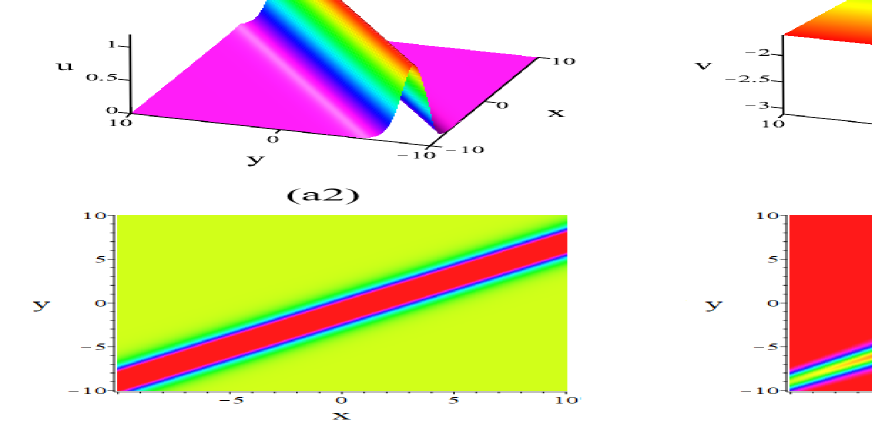
where , and are arbitrary function about and , respectively. To illustrate this solution, we choose =sech, =sech, =sech, =sech and . The figures of and are shown in Figs. 6 (a1), (a2),(b1) and (b2). The interaction between two soliton, with the opposite amplitude in the -direction, and with the same amplitude in the -direction, can be observed.
(4) . Similar computation give the following group-invariant solution
| (4.10) |
where and are arbitrary function of , and is a constant. We choose =sech, =sech, , and , and the resulting solution is shown in Figs. 6 (c1), (c2), (d1) and (d2). The interaction between two solitons, with the same amplitude in the -direction, and with the opposite amplitude in the -direction can be noticed.

(5) . Consider the characteristic equations
| (4.11) |
whose solution give the invariants
| (4.12) |
To conduct the reduction, we choose
| (4.13) |
which are substituted back to (2.5), yielding
| (4.14) |
The reduced system (4.14) is still difficult to be solved immediately. In the following, we will conduct one more step of reduction. As shown in (i) below that the system (4.14) can be reduced to one PDE, and we will conduct the symmetry reduction for (4.14) and the PDE, i.e., (4.16), separately. They are related as local and nonlocal symmetries of differential equations (see, e.g., [8] and references therein).
(i) Symmetries of the PDE (4.16). The first equation of (4.14) can be integrated with respect to , yielding
| (4.15) |
which is then substituted to the second equation. Consequently, the system (4.14) turns into a single PDE
| (4.16) |
where is an arbitrary function.
Remark 4.1.
Expanding the derivatives, Eq. (4.16) reads
| (4.17) |
Lie point symmetries of (4.17) are generated by the infinitesimal generators
| (4.18) |
where we assume .
(i-1) We firstly use to reduce Eq. (4.17), where is constant. The invariants are and , and the Eq. (4.17) is reduced to the third-order ODE
| (4.19) |
Dividing by on both sides and integrating it with respect to , we obtain a second-order ODE
| (4.20) |
By a translation , Eq. (4.20) becomes
| (4.21) |
It is equivalent to the reduced ODE of the KdV equation for searching its traveling wave solutions (see Example 3.4 of [33]), that will appear later, i.e., Eq. (4.35), followed by some special solutions.
(i-2) The invariants with respect to are
| (4.22) |
Now the Eq. (4.17) is reduced to a third-order ODE
| (4.23) |
By the transformation
| (4.24) |
Eq. (4.23) becomes
| (4.25) |
where is a constant of integration. Eq. (4.25) is integrable as passing the Painlevé test and is in the form of Chazy’s classification on third-order Painlevé equations of the polynomial type (see, e.g., Eq. (2.1) of [10]). However, some of the coefficients are locally analytic except . Furthermore, Eq. (4.25) is non-autonomous and seems not included in the 13 classes introduced by Chazy in [9].
Remark 4.2.
If , singularity appears in the symmetries (4.18). Now Eq. (4.17) becomes
| (4.26) |
and its Lie point symmetries are generated by the infinitesimal generators
| (4.27) |
For simplicity, let , and consider that is associated to traveling wave solutions. Choose the invariants as
| (4.28) |
The Eq. (4.26) is reduced to
| (4.29) |
where and is a constant. This ODE is equivalent to (4.20) by a translational transformation of .
In addition, we take , and consider , which corresponding to the scale invariance. The invariants are and , and the Eq. (4.26) is reduced to the third-order ODE
| (4.30) |
Similar to the derivation of Eq. (4.25), introducing , Eq. (4.30) is equivalent to
| (4.31) |
where is a constant of integration. It is again a third-order Painlevé equation of polynomial type, which passes the Painlevé test. It is equivalent to Eq. (4.25) except a term.
(ii) Symmetries of the potential system (4.14). Its Lie point symmetries are generated by
| (4.32) |
where is an arbitrary function.
(ii-1) Consider a special case by taking , and the second generator becomes
| (4.33) |
Consider reductions related to , i.e., traveling wave type of solutions, where is a constant. The invariants are , and , . Now the potential system (4.14) becomes
| (4.34) |
Both equations in (4.34) can be integrated once and the system is equivalent to the following second-order ODE
| (4.35) |
Similar to Eq. (4.20), Eq. (4.35) can also be integrated once, amounting to
| (4.36) |
where are integration constants. If , Eq. (4.35) is equivalent to Eq. (4.21). In the following, we list its special solutions by properly assigning the parameters.
- •
-
•
If we only assume to be bounded similar as [33], Eq. (4.36) has the periodic cnoidal wave solutions
(4.39) where cn is the Jacobi elliptic function of modulus , and are the roots of the cubic polynomial on the right-hand side of Eq. (4.36). The corresponding periodic wave solutions of the system (2.5) are
(4.40) Here, we assumed to be negative.
The traveling wave solutions (4.38) and periodic wave solutions (4.40) of the system (2.5) are shown in Fig. 7 at the time and with variable coefficient . In Figs. 7 (a1), (a2), (b1) and (b2), the parameters are , while in (c1), (c2), (d1) and (d2), the parameters are .
(ii-2) If we choose , then corresponds to the scale invariance, the invariants of which are , , . Then, Eq. (4.14) is reduced to the third-order ODE
| (4.41) |
It is equivalent to Eq. (4.23) by a scaling of providing the constant of integration . If , defining
| (4.42) |
Eq. (4.41) becomes
| (4.43) |
with a constant of integration. It is exactly Eq. (4.31).
(6) . The characteristic equations are
| (4.44) |
solving that gives the invariants
| (4.45) |
We choose the invariant variables as
| (4.46) |
which are substituted into (2.5), yielding
| (4.47) |
5 Conclusions
In this paper, a (2+1)-dimensional integrable KdV system with time-dependent variable coefficient was studied. Its integrability is analyzed by Painlevé analysis. -soliton solutions of the (2+1)-dimensional variable-coefficient KdV system were obtained by using Hirota’s bilinear method. In particular, by choosing appropriate parameters on the -soliton solutions, novel wave interaction phenomena were discovered, e.g., the soliton solutions shown in Figs. 1-2, the hybrid interaction of line, lump and breather solitons illustrated by Fig. 3, the interaction of two breathers (Fig. 4), and the interaction of two lump solutions (Fig. 5). Furthermore, group-invariant solutions are derived by similarity reduction, for instance, an interaction between two solitons in Fig. 6 beside other interesting analytic solutions. These results show interesting novel physical features, which should provide new knowledge in the study of variable-coefficient nonlinear systems. As a final remark, the (2+1)-dimensional integrable variable-coefficient KdV system and the reduced PDE (4.16) are among the few examples that can be reduced to third-order Painlevé equations.
Acknowledgements
L. Peng is grateful to Saburo Kakei, Frank Nijhoff and Ralph Willox for helpful discussions. Y. Liu was partially supported by the National Natural Science Foundation of China (No. 11905013), the Beijing Natural Science Foundation (No. 1222005), and Qin Xin Talents Cultivation Program of Beijing Information Science and Technology University (QXTCP C202118). L. Peng was partially supported by JSPS Kakenhi Grant Number JP20K14365, JST-CREST Grant Number JPMJCR1914, and Keio Gijuku Fukuzawa Memorial Fund.
References
- [1] M. J. Ablowitz and D. E. Baldwin, Nonlinear shallow ocean-wave soliton interactions on flat beaches, Phys. Rev. E 86 (2012), 036305.
- [2] M. J. Ablowitz, D. J. Kaup, A. C. Newell, and H. Segur, The inverse scattering transform-Fourier analysis for nonlinear problems, Stud. Appl. Math. 53 (1974), 249–315.
- [3] M. J. Ablowitz, A. Ramani, and H. Segur, A connection between nonlinear evolution equations and ordinary differential equations of P-type. I, J. Math. Phys. 21 (1980), 715–721.
- [4] O. D. Aseyemo and C. M. Khalique, Analytic solutions and conservation laws of a (2+1)-dimensional generalized Yu-Toda-Sasa-Fukuyama equation, Chinese J. Phys. 77 (2022), 927–944.
- [5] N. Benoudina, Y. Zhang, and C. M. Khalique, Lie symmetry analysis, optimal system, new solitary wave solutions and conservation laws of the Pavlov equation, Commun. Nonlinear Sci. Numer. Simulat. 94 (2021), 105560.
- [6] G. W. Bluman and S. C. Anco, Symmetry and Integration Methods for Differential Equations, Springer, New York, 2002.
- [7] G. Bluman and J. Cole, General similarity solution of the heat equation, J. Math. Mech. 18 (1969), 1025–1042.
- [8] G.W. Bluman, Temuerchaolu, and R. Sahadevan, Local and nonlocal symmetries for nonlinear telegraph equation, J. Math. Phys. 46 (2005), 023505.
- [9] J. Chazy, Sur les équations différentielles du troisième ordre et d’ordre supérieur dont l’intégrale générale a ses points critiques fixes, Acta Math. 34 (1991), 317–385.
- [10] C. M. Cosgrove, Chazy classes IX-XI of third-order differential equations, Stud. Appl. Math. 104 (2000), 171–228.
- [11] M. Boiti, J. P. Leon, M. Manna, and F. Pempinelli, On the spectral transform of a Korteweg-de Vries equation in two spatial dimensions, Inverse Probl. 2 (1986), 271–279.
- [12] J. Chen, Y. Liu, and L. Piao, Various localized nonlinear wave structures in the (2+1)-dimensional KdV system, Modern Phys. Lett. B 34 (2020), 2050128.
- [13] B. F. Feng, R. Ma, and Y. Zhang, General breather and rogue wave solutions to the complex short pulse equation, Physica D 439 (2022), 133360.
- [14] A. S. Fokas, Y. Cao, and J. He, Multi-solitons, multi-breathers and multi-rational solutions of integrable extensions of the Kadomtsev-Petviashvili equation in three dimensions, Fractal Fract. 6 (2022), 425.
- [15] F. Güngör and C. Özemir, Variable coefficient Davey-Stewartson system with a Kac-Moody-Virasoro symmetry algebra, J. Math. Phys. 57 (2016), 063502.
- [16] B. Guo, L. Ling, and Q. P. Liu, Nonlinear Schrödinger equation: Generalized Darboux transformation and rogue wave solutions, Phys. Rev. E 85 (2012), 026607.
- [17] R. Hai and H. Gegen, Rational, semi-rational solution and self-consistent sources extension of the variable-coefficient extended modified Kadomtsev-Petviashvili equation, Phys. Scr. 97 (2022), 095214.
- [18] R. Hirota, The Direct Method in Soliton Theory, Cambridge University Press, Cambridge, 2004.
- [19] P. E. Hydon, Symmetry Methods for Differential Equations: A Beginner’s Guide, Cambridge University Press, Cambridge, 2000.
- [20] M. Jimbo and T. Miwa, Solitons and infinite dimensional Lie algebras, Publ. Res. Inst. Math. Sci. 19 (1983), 943–1001.
- [21] Y. Kodama, KP Solitons and the Grassmannians: Combinatorics and Geometry of Two-Dimensional Wave Patterns, Springer Briefs in Mathematical Physics, Springer, 2017.
- [22] Y. Kuang and J. Zhu, The higher-order soliton solutions for the coupled Sasa-Satsuma system via the -dressing method, Appl. Math. Lett. 66 (2017), 47–53.
- [23] S. Kumar and B. Mohan, A study of multi-soliton solutions, breather, lumps, and their interactions for Kadomtsev-Petviashvili equation with variable time coefficient using Hirota method, Phys. Scr. 96 (2021), 125255.
- [24] R. Li, O. A. İlhan, J. Manafian, K. H. Mahmoud, M. Abotaleb, and A. A. Kadi, Mathematical study of the (3+1)-D variable coefficients generalized shallow water wave equation with its application in the interaction between the lump and soliton solutions, Mathematics 10 (2022), 3074.
- [25] J. Liu, G. Mu, Z. Dai, and H. Luo, Spatiotemporal deformation of multi-soliton to (2+1)-dimensional KdV equation, Nonlinear Dyn. 83 (2016), 355–360.
- [26] J. G. Liu, L. Zhou, and Y. He, Multiple soliton solutions for the new (2+1)-dimensional Korteweg-de Vries equation by multiple exp-function method, Appl. Math, Lett. 80 (2018), 71–78.
- [27] Y. Liu, B. Ren, and D. S. Wang, Localised nonlinear wave interaction in the generalised Kadomtsev-Petviashvili equation, E. Asian J. Appl. Math. 11 (2021), 301–325.
- [28] Y. Liu, X. Y. Wen, and D. S. Wang, Novel interaction phenomena of localized waves in the generalized (3+1)-dimensional KP equation, Comput. Math. Appl. 78 (2019), 1–19.
- [29] A. V. Mikhailov, G. Papamikos, and J. P. Wang, Dressing method for the vector sine-Gordon equation and its soliton interactions, Physica D 325 (2016), 53–62.
- [30] A. V. Mikhailov, V. V. Sokolov, and A. B. Shabat, The symmetry approach to classification of integrable equations, in: What is Integrability? (V.E. Zakharov, ed.), Springer, Berlin, 1991, pp. 115–184.
- [31] R. A. Mohamed, W. X. Ma, and R. Sadat, Lie symmetry analysis and wave propagation in variable-coefficient nonlinear physical phenomena, E. Asian J. Appl. Math. 12 (2022), 201–212.
- [32] R. A. Mohamed and R. Sadat, Lie symmetry analysis, new group invariant for the (3+1)-dimensional and variable coefficients for liquids with gas bubbles models, Chinese J. Phys. 71 (2021), 539–547.
- [33] P. J. Olver, Applications of Lie Groups to Differential Equations, 2nd ed., Springer, New York, 1993.
- [34] P. J. Olver, Evolution equations possessing infinitely many symmetries, J. Math. Phys. 18 (1977), 1212–1215.
- [35] P. J. Olver and P. Rosenau, Group-invariant solutions of differential equations, SIAM J. Appl. Math. 47 (1987), 263–278.
- [36] M. S. Osman, One-soliton shaping and inelastic collision between double solitons in the fifth-order variable-coefficient Sawada-Kotera equation, Nonlinear Dyn. 96 (2019), 1491–1496.
- [37] L. Peng, Symmetries, conservation laws, and Noether’s theorem for differential-difference equations, Stud. Appl. Math. 139 (2017), 457–502.
- [38] J. Rao, D. Mihalache, and J. He, Dynamics of rogue lumps on a background of two-dimensional homoclinic orbits in the Fokas system, Appl. Math. Lett. 134 (2022), 108362.
- [39] J. Satsuma and M. J. Ablowitz, Two-dimensional lumps in nonlinear dispersive systems, J. Math. Phys. 20 (1979), 1496–1503.
- [40] B. K. Shivamoggi, The Painlevé analysis of the Zakharov-Kuznetsov equation, Physica Scr. 42 (1990), 641–642.
- [41] T. Trogdon and B. Deconinck, Numerical computation of the finite-genus solutions of the Korteweg-de Vries equation via Riemann-Hilbert problems, Appl. Math. Lett. 26 (2013), 5–9.
- [42] C. Wang, Spatiotemporal deformation of lump solution to (2+1)-dimensional KdV equation, Nonlinear Dyn. 84 (2016), 697–702.
- [43] A. M. Wazwaz, Painlevé analysis for new (3+1)-dimensional Boiti-Leon-Manna-Pempinelli equations with constant and time-dependent coefficients. Int. J. Numer. Methods Heat Fluid Flows 30 (2019), 4259–4266.
- [44] G. M. Wei, Y. L. Lu, Y. Q. Xie, and W. X. Zheng, Lie symmetry analysis and conservation law of variable-coefficient Davey-Stewartson equation, Comput. Math. Appl. 75 (2018), 3420–3430.
- [45] X. Y. Wu and Y. Sun, Dynamic mechanism of nonlinear waves for the (3+1)-dimensional generalized variable-coefficient shallow water wave equation, Phys. Scr. 97 (2022), 095208.
- [46] Y. Xia, R. Yao, and X. Xin, Nonlocal symmetries and group invariant solutions for the coupled variable-coefficient Newell-Whitehead system, J. Nonlinear Math. Phys. 27 (2020), 581–591.
- [47] X. X. Xu and Y. P. Sun, An integrable coupling hierarchy of Dirac integrable hierarchy, its Liouville integrability and Darboux transformation, J. Nonlinear Sci. Appl. 10 (2017), 3328–3343.
- [48] F. Yu and R. Fan, Nonstandard bilinearization and interaction phenomenon for PT-symmetric coupled nonlocal nonlinear Schrödinger equations, Appl. Math. Lett. 103 (2020), 106209.
- [49] W. X. Zhang and Y. Liu, Integrability and multisoliton solutions of the reverse space and/or time nonlocal Fokas-Lenells equation, Nonlinear Dyn. 108 (2022), 2531–2549.
- [50] Y. Zhang, Y. Liu, and X. Tang, M-lump solutions to a (3+1)-dimensional nonlinear evolution equation, Comput. Math. Appl. 76 (2018), 592–601.