Multiple polaron quasiparticles with dipolar fermions in a bilayer geometry
Abstract
We study the Fermi polaron problem with dipolar fermions in a bilayer geometry, where a single dipolar particle in one layer interacts with a Fermi sea of dipolar fermions in the other layer. By evaluating the polaron spectrum, we obtain the appearance of a series of attractive branches when the distance between the layers diminishes. We relate these to the appearance of a series of bound two-dipole states when the interlayer dipolar interaction strength increases. By inspecting the orbital angular momentum component of the polaron branches, we observe an interchange of orbital character when system parameters such as the gas density or the interlayer distance are varied. Further, we study the possibility that the lowest energy two-body bound state spontaneously acquires a finite center of mass momentum when the density of fermions exceeds a critical value, and we determine the dominating orbital angular momenta that characterize the pairing. Finally, we propose to use the tunneling rate from and into an auxiliary layer as an experimental probe of the impurity spectral function.
I Introduction
Over the last two decades, significant progress has been made in manipulating ultracold gases of dipolar atoms and molecules. The surge in experimental activity in this field is motivated by the expectation that the anisotropic and long-range nature of dipole-dipole interactions can lead to exotic states of matter Lahaye et al. (2009); Baranov et al. (2012); Chomaz et al. (2022). Significant progress has already been made with dipolar gases of highly magnetic atoms such as Cr Griesmaier et al. (2005); Stuhler et al. (2005), Dy Lu et al. (2011, 2012), and Er Aikawa et al. (2012, 2014a), where the achievement of quantum degeneracy has allowed the investigation of droplets, supersolids and other quantum phenomena Böttcher et al. (2020). However, in order to access the regime of strong dipole-dipole interactions, one requires other cold-atom platforms such as Rydberg atoms Löw et al. (2012) or heteronuclear molecules Moses et al. (2017); Shaffer et al. (2018).
Fermionic polar molecules in layered geometries are particularly promising for realizing quantum phases with strong and tunable dipolar interactions. By confining dipolar molecules to two-dimensional (2D) layers, inelastic losses are suppressed, while the sign and strength of the dipolar interactions can be precisely controlled Valtolina et al. (2020). Degenerate 2D Fermi gases have already been achieved with KRb Marco et al. (2019); Tobias et al. (2020) and NaK Schindewolf et al. (2022); Duda et al. (2023), while other molecules, including LiCs Deiglmayr et al. (2008); Repp et al. (2013) and NaLi Park et al. (2023), are also being explored. Moreover, recent experiments with ultracold KRb molecules have demonstrated the possibility to image and control multiple layers individually Tobias et al. (2022), thus expanding the range of scenarios that can be explored with 2D dipolar gases.
From a theoretical standpoint, dipole-dipole interactions are expected to generate ordered phases of fermions in layered geometries. Of particular interest is the configuration where all dipole moments are aligned perpendicularly to the confining planes, such that the system has rotational symmetry. In the case of a single layer, intralayer superfluid -wave pairing can be driven by dressing polar molecules with a microwave field Cooper and Shlyapnikov (2009); Levinsen et al. (2011). Furthermore, density-wave instabilities with dipolar fermions have been proposed Bruun and Taylor (2008); Yamaguchi et al. (2010); Sun et al. (2010), including the spontaneous appearance of a stripe phase Parish and Marchetti (2012) and Wigner crystallization Matveeva and Giorgini (2012) at sufficiently high densities or strong interactions. In the case of bilayers, in addition to density-wave instabilities Marchetti and Parish (2013), new interlayer bound pairs can arise due to the attractive part of the dipolar interaction Klawunn et al. (2010a); Potter et al. (2010); Pikovski et al. (2010); Klawunn et al. (2010b). Such pairing and associated interlayer superfluidity has been studied in the case of both balanced Bruun and Taylor (2008); Pikovski et al. (2010); Mazloom and Abedinpour (2018) and imbalanced populations Mazloom and Abedinpour (2017). The latter includes the possibility of realizing a Fulde-Ferrell-Larkin-Ovchinnikov (FFLO) modulated pairing phase Lee et al. (2017). Most notably, the stability of the FFLO state can be enhanced by the long-range character of the interlayer dipolar interaction, where different partial waves contribute to the pairing order parameter.
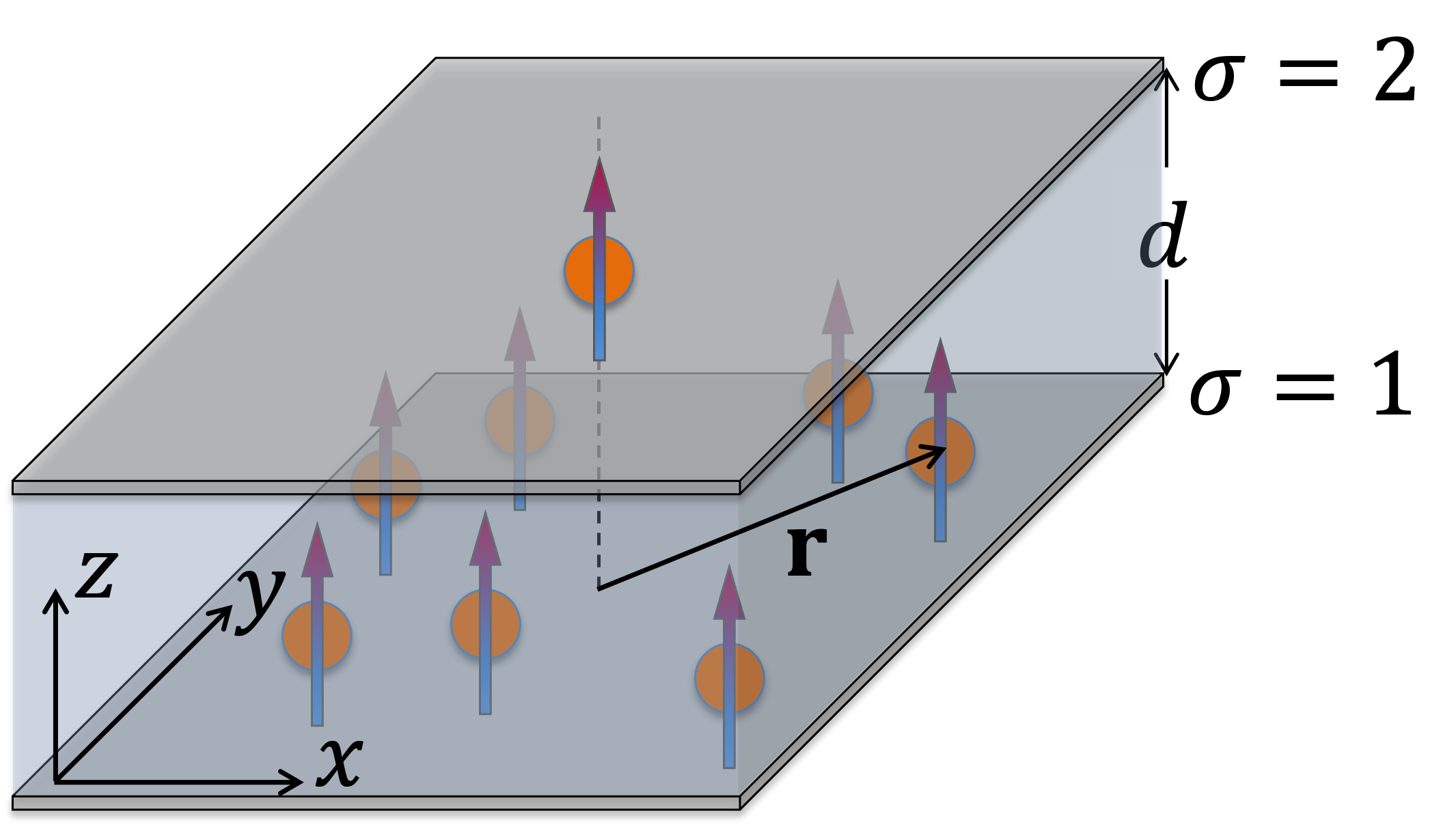
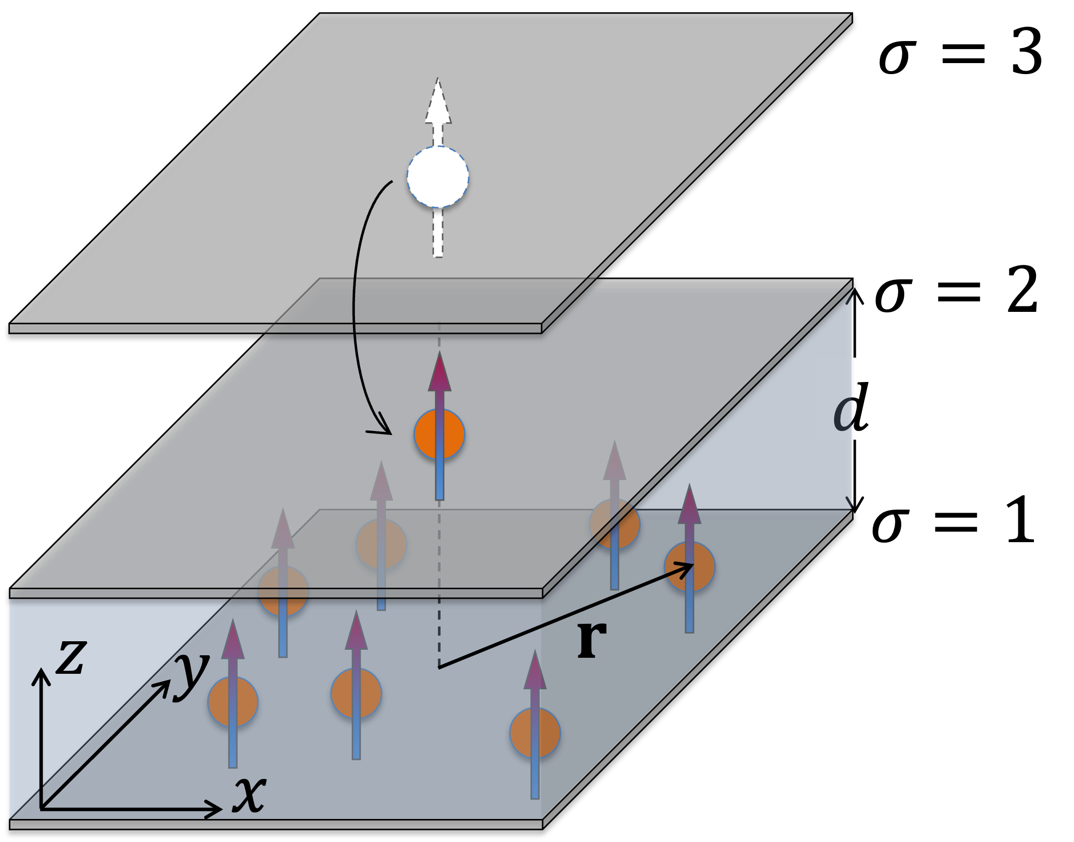
In this work, we consider the limit of extreme population imbalance for dipolar fermions in a bilayer, as illustrated in Fig. 1. Specifically, we have an impurity problem, where a single dipolar particle in one layer interacts with a Fermi sea of identical dipolar fermions in a different layer. This so-called “Fermi-polaron” problem has previously been considered in Refs. Klawunn and Recati (2013); Matveeva and Giorgini (2013) for the case of dipoles in a bilayer geometry 111The “repulsive Fermi polaron” problem with dipolar fermions in a single layer geometry has been considered in Ref. Bombín et al. (2019)., and the general problem of an impurity in a 2D Fermi gas has been extensively studied in other 2D platforms such as ultracold atoms Zöllner et al. (2011); Parish (2011); Schmidt et al. (2012a); Ngampruetikorn et al. (2012); Parish and Levinsen (2013); Tajima et al. (2021) and doped semiconductors Sidler et al. (2016); Efimkin et al. (2021); Tiene et al. (2022); Huang et al. (2023). Our scenario can be readily realized with polar molecules; however, note that our setup is quite general and could in principle apply to other dipoles such as Rydberg atoms. We consider two possible solutions of this problem. In the first, we generalize the interlayer bound state between two dipoles to include the effects of an inert Fermi sea and how it blocks the occupation below the Fermi momentum. In the second, we consider the possibility of “polaron” quasiparticles, where the impurity is dressed by particle-hole excitations of the Fermi sea. Throughout, we compare our results with those previously obtained within a -matrix formalism which focused on the limit of weak dipolar interactions Klawunn and Recati (2013).
By employing a variational Ansatz, we evaluate the polaron spectrum to reveal that it is characterized by a series of attractive polaron branches, where the number of branches increases when the distance between the two layers decreases or the dipole moment increases. We associate the appearance of these polaron branches to the series of two-body bound states that, similarly to the 2D hydrogen atom Yang et al. (1991), is characterized by a specific orbital angular momentum component and a principal quantum number. In the limit of vanishingly small density of fermions, the attractive polaron energies recover those of the dipole-dipole bound states. By evaluating the orbital angular momentum component of each polaron branch, we observe that the partial wave character of the branches evolve and interchange when we either increase the Fermi density or, at a fixed density, we increase the bilayer distance.
In contrast to the well-studied case of contact impurity-medium interactions Massignan et al. (2014); Scazza et al. (2022), a distinctive feature of finite-range dipole-dipole interactions is that the energy of the lowest energy polaron branch can either redshift, i.e., lower its energy, with increasing Fermi density, or blueshift. We find that this depends on the precise value of the dipolar strength, a quantity related to the specific value of the dipole moment and the layer separation. We explain this qualitative different behavior in terms of the contribution of hole scattering in the polaron formation, which we find is particularly important for the dipolar potential.
Further, we consider the possibility that the lowest dipole-dipole bound state spontaneously acquires a finite center of mass momentum when the density of the Fermi sea increases. Because of the long-range nature of the dipole-dipole interaction, this finite-momentum bound state mixes different orbital angular momentum components. We show that, while for small densities, -wave pairing dominates close to the transition, for larger densities, the bound state acquires - and -wave components. These results agree with those found at finite but large imbalance in Ref. Lee et al. (2017).
The paper is organized as follows. In Sec. II we introduce the model of identical dipolar fermions in a bilayer geometry, and we discuss the relevant length and energy scales including their typical values in current experiments for either strongly magnetic atoms or heteronuclear molecules. Section III describes the properties of the two-body interlayer bound states, generalized to the case where a Fermi gas in one of the layers acts to block the occupation of states below the Fermi sea. In Sec. IV we describe the spectral properties of the Fermi polaron, while in Sec. V we show that the polaron spectral function can be probed analogously to radiofrequency spectroscopy by introducing an auxiliary layer to the system. Conclusions and perspectives are gathered in Sec. VI.
II Model
We investigate the configuration schematically represented in Fig. 1. A Fermi sea of dipoles (e.g., polar molecules) is confined in one layer, with index , where the dipole moments of the molecules are aligned perpendicularly to the plane by an external field. Additionally, a single dipolar molecule with the same perpendicular alignment occupies layer . The Hamiltonian describing the systems is (we set and the system area ):
| (1) |
where () is the creation (annihilation) operator of a fermionic dipole with momentum in layer . Dipoles in different layers have the same mass and their kinetic energy is .
In writing Eq. (1) we have implicitly assumed that the intralayer correlations are weak, such that the gas in layer is in a Fermi liquid phase where it can be treated as approximately non-interacting. This neglects the possibility of density instabilities which can occur in a (perpendicularly alligned) 2D dipolar Fermi gas with large dipole moments or high densities Parish and Marchetti (2012).
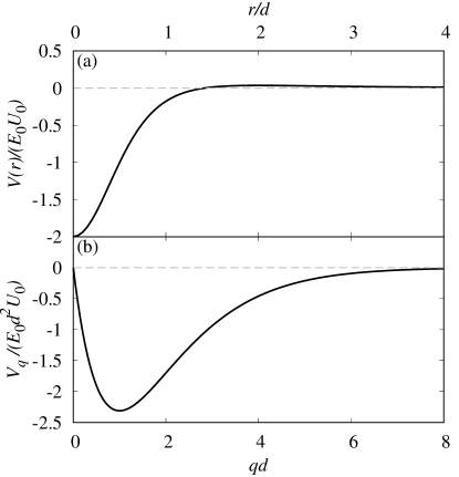
On the other hand, the second term in the Hamiltonian (1) describes the dipolar interaction between a molecule in layer and one in layer . The interlayer dipolar potentials in real and momentum space are, respectively, given by Pikovski et al. (2010); Li et al. (2010); Klawunn et al. (2010b):
| (2a) | ||||
| (2b) | ||||
where is the planar separation. Here is the layer separation and is the dipolar interaction strength. Out of these variables it is profitable to introduce a dimensionless dipolar strength
| (3) |
where is the energy scale associated with the layer separation. We see that increases by either increasing the dipolar interaction strength or by moving the two layers closer to each other.
The interlayer dipolar potential is plotted in Fig. 2 in real and momentum space. As expected, in real space the potential is attractive at short distances , where the dipoles are effectively arranged head-to-tail, while it is repulsive at large distances , where the dipoles are arranged side-by-side. Note that the interlayer potential has a vanishing zero-momentum contribution, i.e.,
This implies that the two-dipole bound state becomes very shallow when Klawunn et al. (2010b), as discussed further in Sec. III.
The dipolar interaction strength , which has the dimensions of energy times volume, is related to either the permanent magnetic dipole moment of a magnetic atom or to the dipole moment of an atom or a molecule induced by an electric field Lahaye et al. (2009):
where is the vacuum permeability and the vacuum permittivity. Usually heteronuclear molecules with induced electric dipole moments display much stronger dipole-dipole interactions than atoms with a permanent magnetic moment. In order to quantify the dipolar interaction, it is convenient to introduce the dipolar length Lahaye et al. (2009); Chomaz et al. (2022) 222Note that Refs. Lahaye et al. (2009); Chomaz et al. (2022) use a different definition of but the same definition of : . :
| (4) |
For heteronuclear molecules, can be up to 3 orders of magnitude larger than for magnetic atoms. Typical values of for the highly magnetic atom 164Dy and for the heteronuclear molecules KRb and LiCs are given in Table 1. Furthermore, in current experiments, typically nm; however very recently a new super-resolution technique which localizes and arranges dipolar molecules on a sub- nm scale has been implemented Du et al. (2023). The corresponding values of that can be achieved for both highly magnetic atoms and heteronuclear molecules are listed in Table 1. Throughout this work we consider the dipoles to be structureless fermions such that we do not make a distinction between magnetic atoms or heteronuclear molecules.
| 164Dy | 130.7 | 0.4 | 0.04 | 0.07 |
| KRb | 6.3 | 0.6 | 1.1 | |
| LiCs | 634.8 | 63.5 | 110 |
The density of dipoles in layer is related to the Fermi momentum by
| (5) |
From this, we can define a many-body dimensionless parameter analogous to the dipolar strength :
| (6) |
This dimensionless interaction strength characterizes the extent of many-body correlations in the system. As discussed above, we neglect the intralayer interaction and assume an ideal Fermi gas in layer . Strictly speaking, this requires us to consider sufficiently small values of such that there are no ordered phases. Specifically, in the case of perpendicular orientation of the dipole moments, it has been found that the translational symmetry is broken for towards the appearances of a stripe phase Parish and Marchetti (2012), while Wigner crystallization can occur for Matveeva and Giorgini (2012). Nevertheless, to comprehensively characterize bound-state and polaron properties in the presence of a Fermi gas, we must extend our investigation to higher density values. Therefore, to preserve the assumption of an ideal Fermi gas in layer , we will implicitly assume that there is a small but finite temperature that induces the melting of the strongly correlated phases without strongly affecting the impurity physics.
Typically, the density of the 2D Fermi gas in experiments is cm-2. This leads to values of listed in the fourth column of Table 1. We furthermore list typical values for the dimensionless parameters and at different bilayer separation in Table 2.
| nm | nm | |
|---|---|---|
| 0.015 | 1.6 | |
| 5.7 | 0.56 |
III Dimer states
Due to the attractive part of the dipolar interaction, two dipoles can form an interlayer bound state. In this section, we discuss the properties of this two-body bound (dimer) state, generalized to the case where the Fermi gas in layer is inert and acts to block the occupation below the Fermi momentum . We thus consider a general two-body state with a center-of-mass momentum described by:
| (7) |
where the sum over the relative momenta is restricted by Pauli blocking, , while describes the Fermi sea in layer 1, and is the two-body wavefunction. The energies can then be found by solving the corresponding Schrödinger equation:
| (8) |
which can be readily solved by numerical diagonalization.
Before discussing the solution of Eq. (8), it is useful to classify the dimer states according to their orbital angular momentum component. First, if the impurity momentum , the system is rotationally symmetric, and angular momentum is a good quantum number. Furthermore, when , the center of mass and relative motion decouple, and therefore the energy at finite is simply related to the energy at via , allowing us to take advantage of the rotational symmetry at . The presence of the Fermi sea complicates matters because then the center of mass motion no longer decouples. Thus, for a dimer state where both and are finite, the system is no longer rotationally invariant and orbital angular momentum is not conserved.
To proceed, we expand the dimer wavefunction as a Fourier series over the orbital angular momentum basis :
| (9) |
where is the angle between and . The dimer Schrödinger equation (8) now reads
| (10) |
Here, we have taken the continuum limit, and decomposed the interlayer potential in the orbital angular momentum basis by using the fact that the potential is diagonal in angular momentum, i.e.,
| (11) |
where and . Note that the potential is real.
As expected, Eq. (10) becomes diagonal in when since, in this limit, the orbital angular momentum is a good quantum number. Note also that, because the potential is symmetric under the exchange , the eigenvectors for can either be symmetric or antisymmetric solutions:
| (12) |
where , while . In terms of these, the Schrödinger equation reads ():
| (13) |
One can see that the Schrödinger equation (10) now becomes block diagonal using the symmetric and antisymmetric dimer wavefunctions, i.e., the equations for and decouple from those for , the former states being in general the lowest energy solutions 333Note that, as mentioned previously, the Schrödinger equation becomes diagonal in when either or , such that symmetric and antisymmetric solutions become degenerate..
In the following two subsections, we first analyze the two-body limit, i.e., the limit where there is a single particle in each of layers and , and we study the appearance of additional bound dimer states when the interlayer dipolar strength increases. Then, in Sec. III.2, we consider the effect of a finite density of fermions in layer and how this can lead to the dimer spontaneously acquiring a finite center of mass momentum.
III.1 Vacuum dimer
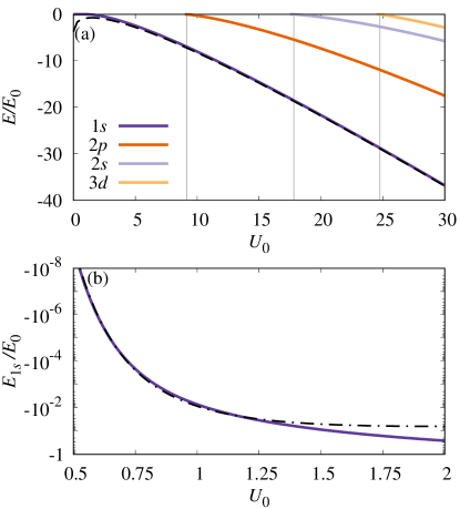
As explained above, in the absence of a Fermi sea in layer 1, the center-of-mass and relative motion decouple. We therefore solve the two-body problem at . The dimer states can be labelled by the orbital angular momentum and the eigenvalue index (where increasing values of indicate larger energies eigenstates), which we assume to be , in analogy with the 2D hydrogenic atom Yang et al. (1991).
We plot in Fig. 3 the energies of the dimer states for increasing values of , i.e., for either increasing values of the dipole moments or smaller bilayer distances . As expected, the state is always bound for , even if it becomes very shallow when , i.e., the binding energy goes exponentially to zero. This has been already analyzed by Ref. Klawunn et al. (2010b) and traced back to the fact that the interlayer dipolar potential has a vanishing zero-momentum contribution, in which case one cannot use Landau’s formula for the energy of the bound state . Instead, Ref. Klawunn et al. (2010b) found an approximation for the energy when by employing the Jost function formalism, leading to:
| (14) |
where is the Euler-Mascheroni constant. For large values of , variational calculations Yudson et al. (1997) show that
| (15) |
We see that these perturbative expressions match well with our numerical results in the two limits, as shown in Fig. 3.
In addition to the bound state, we find that the interlayer dipolar potential can bind an increasing number of dimer states with increasing . The corresponding thresholds are indicated as grey vertical lines in Fig. 3 and are listed in Table 3. In order of increasing , the sequence of additional dimer states that eventually bind is , , , , , , , . Note that this order can change when we introduce the effects of Pauli blocking at finite , even though the orbital angular momentum remains a good quantum number for .
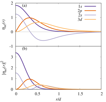
For each bound state with energy , we evaluate in Fig. 4 the corresponding dimer eigenfunctions in real space,
| (16) |
where is the Bessel function of the first kind. We find that, at small distances , the dimer wavefunctions can be well approximated as
| (17a) | ||||
| (17b) | ||||
| (17c) | ||||
| (17d) | ||||
This is similar to the hydrogenic atom in 2D Yang et al. (1991), with the difference being that the dipolar potential leads to a stronger confinement to shorter distances than the Coulomb potential, i.e., the wavefunctions are concentrated at .
Apart from the two-body bound states, we might wonder about the scattering properties of the interlayer dipolar potential (2). In particular, one can show Klawunn et al. (2010b) that there is only a very restricted parameter regime of scattering energies and values of where the scattering properties of the dipolar potential recover those of a short-range contact-like attractive potential. This, as also discussed in Ref. Klawunn et al. (2010b), is due to the fact that for the potential leads to a very shallow bound state, while for there are additional states becoming bound. We discuss these aspects in App. A, where we explicitly evaluate the scattering phase shift within the variable-phase method.
III.2 Finite and finite- dimers
Similarly to the case of other attractive interaction potentials, the dimer ground state spontaneously acquires a finite center-of-mass momentum above a threshold density of fermions Parish et al. (2011); Parish and Levinsen (2013); Cotlet et al. (2020); Tiene et al. (2020). Such a dimer state can be regarded as the extreme imbalance limit of the FFLO phase in spin-imbalanced superconductors Fulde and Ferrell (1964); Larkin and Ovchinnikov (1964). Over the last few decades there has been significant interest in studying this inhomogeneous superfluid phase in a variety of physical systems – see, e.g., recent reviews Casalbuoni and Nardulli (2004); Radzihovsky and Sheehy (2010). The possibility of generating such a phase has already been studied in Ref. Lee et al. (2017) for fermionic dipolar molecules in a bilayer geometry with a finite imbalance of layer densities. Here, it was found that, when the imbalance exceeds a critical value, the system undergoes a transition from a uniform interlayer superfluid phase to the FFLO phase and that this phase is enhanced by the long-range character of the interlayer dipolar interaction. Indeed, it has previously been shown that unscreened Coulomb interactions significantly stabilizes the FFLO phase Parish et al. (2011).
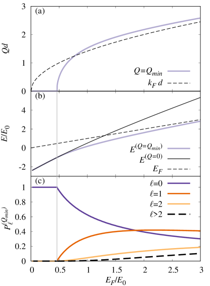
In this section, we consider this problem from the perspective of the extremely imbalanced limit, with a single particle in layer . We show in Fig. 5 the spontaneous formation of a dimer state with finite center-of-mass momentum for the specific case of . In this case, we observe that the dimer state has a minimum at for . For larger densities of the Fermi sea in layer , the lowest energy solution is for , with energy , in which case the orbital angular momentum ceases to be a good quantum number. For the range of studied in this work (), we do not observe any unbinding of the finite dimer state, i.e., we find that the dimer energy remains below the energy of the normal state .
As also commented in Ref. Lee et al. (2017), the long-range nature of the dipole-dipole interaction can mix different angular momentum components of the paired state and thus enhance the FFLO regime. We evaluate the probability that the lowest energy dimer eigenstate contains an orbital angular momentum component as
| (18) |
We plot as a function of in Fig. 5(c). When , the lowest energy state is because is a good quantum number. However, for where the lowest dimer state develops a minimum at , the lowest eigenvalue is characterized by several orbital angular momentum components . As the transition from to finite is second order, the component () dominates close to the transtion. For larger values of , the dimer state acquires first a -wave component () and, later, a smaller contribution from the , as well as components.
In the following section, we illustrate how the properties of the ground and excited states of the two-body bound dimers affect the polaron properties, including its spectral function.
IV Polaron
We now analyze the spectral properties of the polaron formed by the dipolar impurity in layer which is dressed by particle-hole excitations of the Fermi sea of dipoles in layer . To this end, we employ a variational ansatz Chevy (2006) describing a polaron with zero center-of-mass momentum as the superposition between the bare impurity weighted by the variational parameter and a single particle-hole excitation, described by :
| (19) |
Here, we use a notation where is the momentum of the particle states () and of the hole states (). The polaron state is normalized so that .
The variational ansatz in Eq. (19) has previously been successfully employed to describe the impurity problem in different contexts, including ultracold atoms Zöllner et al. (2011); Parish (2011); Schmidt et al. (2012a); Ngampruetikorn et al. (2012); Parish and Levinsen (2013) and doped semiconductors Sidler et al. (2016); Efimkin et al. (2021); Tiene et al. (2022); Huang et al. (2023). In the case of contact interactions, truncating the dressing of the Fermi sea to a single particle-hole excitation has been demonstrated to be an excellent approximation, with an almost exact cancellation of higher order contributions Combescot and Giraud (2008).
Previous work on the dipolar case Klawunn and Recati (2013) employed a -matrix approach to evaluate the lowest attractive polaron branch energy, but the entire spectrum of excitations and the important role played by excited dimer states have not previously been considered. Furthermore, we find that there are important qualitative differences between the variational ansatz (19) and the -matrix approach. This is unlike the case of a pure contact interaction, where the variational ansatz in Eq. (19) is completely equivalent to the -matrix approach within a ladder approximation Combescot et al. (2007). This highlights the important role played by the longer-range parts of the dipolar interaction potential, despite the dipole-dipole interaction formally corresponding to a short-range interaction in the sense that one can define an asymptotic region and an associated 2D scattering length Baranov et al. (2011). We discuss in App. B the precise relation between the ansatz (19) and the -matrix approach employed in Ref. Klawunn and Recati (2013).
By minimizing the expectation value with respect to the variational parameters and , the polaron spectral properties can be found by solving the eigenvalue problem
| (20a) | ||||
| (20b) | ||||
where and where we have omitted the terms that are zero because . The polaron spectral function can be evaluated as usual from the impurity Green’s function Mahan (2000):
| (21a) | ||||
| (21b) | ||||
Similarly to the dimer problem, it is profitable to project the eigenvalue problem (20) onto an eigenbasis of the orbital angular momentum. This simplifies the numerical solution considerably, because we will see that the polaron branches are characterized by a small number of partial waves . Thus, we consider the following Fourier series of the dimer-hole wavefunctions:
The eigenvalue equations in (20) now read:
| (22a) | ||||
| (22b) | ||||
where we have employed Eq. (11). As for the dimer wavefunction, it is convenient to introduce symmetric and antisymmetric solutions for the exchange :
| (23) |
where and . Restricting to , the eigenvalue equations become
| (24a) | ||||
| (24b) | ||||
We thus find that the equations for symmetric and antisymmetric dimer-hole wavefunctions decouple. Most importantly, the impurity wavefunction only couples to the symmetric dimer-hole wavefunction . Thus, the antisymmetric solutions will lead to additional eigenvalues for the polaron problem but these will all have zero spectral weight. As such, we can halve the degrees of freedom in the problem by neglecting the antisymmetric sector.
By discretizing the eigenvalue equations on a Gauss-Legendre grid in and and including a finite number of values , we numerically diagonalize Eq. (24) to find eigenvalues and eigenvectors and thus evaluate the polaron spectral function according to Eq. (21). We have checked that all our results are numerically converged with respect to the number of points in the momentum grids as well as in the number of values. It is interesting to note that when we need only very few, around 4, values of to obtain converged results in the considered parameter regime, while to describe the scattering states we find that values of are sufficient.
IV.1 Spectral properties
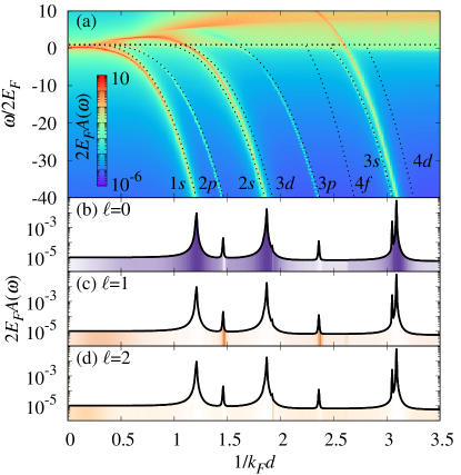
We plot the polaron spectral function as a function of energy and Fermi gas density in Figs. 6, 8, and 10, for three increasing values of . We see that there are strong qualitative differences between the spectra, which originate from the different numbers and types of dimer bound states. We now go through these in detail.
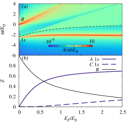
Let us first discuss the case , corresponding to Fig. 6, for which only the two-body dimer state is bound (see Fig. 3). The spectrum in Fig. 6(a) is characterized by two polaron branches and a continuum of states. For , the attractive polaron branch recovers the energy of the dimer state in the limit , and we thus label it as the attractive branch. This resonance is well separated from the continuum, and its energy coincides with the lowest energy-eigenvalue of Eq. (24). The polaron spectrum also exhibits another resonance at , the repulsive polaron, which corresponds to a continuum of states rather than being characterized by a single eigenvalue. When , the repulsive polaron recovers the energy of the bare impurity at rest, , while it blueshifts when increases. Simultaneously, it broadens and loses spectral weight. In between the attractive and repulsive branches is a continuum of states where the hole in the complex of the polaron state (19) is unbound, while the dimer is bound. The energy of such a state is that of a dimer with center-of-mass momentum and a hole at momentum , and hence the boundaries of this dimer-hole continuum are and , respectively, where the energy is computed using Eq. (12) 444Note that we only plot the dimer energy at finite center of mass corresponding to the symmetric states under the exchange in Eq. (12) since these are the only ones with finite spectral weight. Instead, for zero center of mass momentum, symmetric and antisymmetric solution are degenerate in energy.. Both energies recover when , as expected.
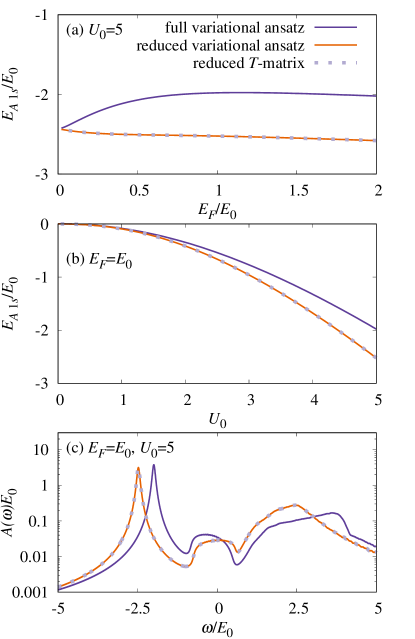
A distinctive feature of the spectrum in Fig. 6(a) is that the attractive branch blueshifts (increases its energy) as we increase . This is in contrast to the case of contact interactions Schmidt et al. (2012b); Ngampruetikorn et al. (2012) where the attractive branch always redshifts (lowers its energy) with increasing . The origin of this qualitatively new feature is that the dipole-dipole scattering can be significant at low momenta [see Fig. 2(b)] and therefore the hole scattering can be strongly enhanced relative to particle scattering despite the reduced phase space. As also discussed in App. B, we can specifically trace the difference to the term in Eq. (20), which is not present in the previous -matrix treatment of the dipolar polaron problem Klawunn and Recati (2013). This term is negligible for , in which case the attractive branch redshifts when increases, but it becomes important for larger values of . The change from redshift to blueshift with increasing is shown in Fig. 7, where we plot the evolution with of the energy of the attractive branch measured from the vacuum dimer energy, .
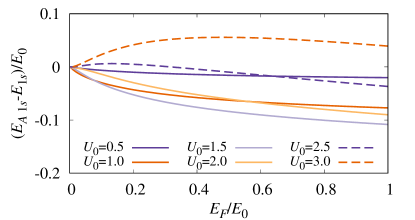
Figure 6(b) shows the spectral weight for each of the branches, which is defined as the area of the spectral function under the corresponding peak. Because the eigenvectors of the polaron problem form a complete basis, the spectral function satisfies the sum rule , and thus the total spectral weight is always 1 for all interaction strengths and densities. When , the spectral weight belongs entirely to the repulsive polaron branch, which coincides with the non-interacting impurity. When increases, we see that is transferred mostly to the attractive branch, first linearly and then sublinearly. Only a small part of the spectral weight is transferred to the dimer-hole continuum.
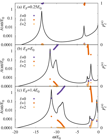
In Fig. 8 we show the case of stronger interactions at which also the dimer state 2 is bound (see Fig. 3). Now, the impurity spectrum changes qualitatively from the previous case because there are two attractive polaron branches: when , one recovers, as before, the energy of the dimer state, , while the second branch recovers the energy of the dimer state, . Here, we label the attractive polaron resonances by and even though their orbital angular momentum components evolve with and change in character (see below). Both attractive resonances have an associated dimer-hole continuum: as before, the boundaries of these are the energies of the dimer states and 555Note that only for the state do we always have .. While the dimer-hole continuum is higher in energy than the attractive branch, we find that this is not necessarily the case for the branch, which for clearly appears above its dimer-hole continuum (for , the spectral weight is very small and it is difficult to distinguish it from its dimer-hole continuum). Both the attractive branch and the continuum blueshift in energy for increasing and, eventually, move into the continuum of the dimer state at .
Figure 8(a) also shows how the spectral weight of the repulsive branch is predominantly transferred to the -wave-like attractive branch and how, compared with the case of in Fig. 6, the spectral weight is transferred more slowly because the state is deeper bound. As a result, the repulsive branch remains brighter and broadens more slowly for increasing than in the previous case. This is further analyzed in Fig. 8(b), where we see that the attractive branch spectral weight grows linearly with for small , while the attractive branch spectral weight grows sublinearly and remains very small. Note that, with increasing density, the attractive branch enters the continuum (vertical gray line in Fig. 8), in which case the criterion that we employ to evaluate the spectral weight of both the attractive and repulsive branches becomes inapplicable due to the rapid broadening of both modes. In Fig. 8(b), we thus stop plotting their spectral weights at this point.
To gain further insight into the angular momentum structure of the polarons, we can evaluate the probability that the hole in a given dimer-hole eigenstate has an orbital angular momentum component Tiene et al. (2022):
| (25) |
Because only the symmetric states (23) have a finite spectral weight, the probability satisfies . Further, the probability is normalized such that . In Fig. 9, we plot the polaron spectral function for for different values of together with the probability for as a function of (with the dots corresponding to discrete eigenvalues). One can clearly see that, for , the eigenvalues corresponding to the attractive branch and its continuum are predominantly -wave, i.e., , while , and the eigenvalues corresponding to the attractive branch and its continuum are predominantly -wave, i.e. , while . However, for larger values of , there is an evolution of these probabilities, where the branch acquires a -wave component, while the branch acquires both - and -wave components. As far as the dimer-hole continuum is concerned, as already discussed in Sec. III, the dimer state at zero center of mass corresponds to a single value of the orbital angular momentum . This can be clearly seen in Fig. 9, where we recognize the energies of the dimer at zero center of mass limiting the dimer-hole continua, as those having , with either or . However, for the other boundary of the dimer-hole continua, , the dimer state at finite center-of-mass momentum is generally not an eigenstate of the orbital angular momentum and involves a mixture of values that evolve with .
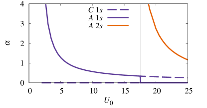
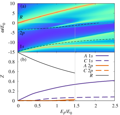
In Fig. 10 we plot the spectrum for strong dipolar interactions, , for which also the dimer state becomes bound. Here, the repulsive branch very quickly transfers its spectral weight to the nearby attractive branch — see Fig. 10(b). The behavior of the attractive branch is very similar to the case analyzed previously. On the other hand, the attractive branch now becomes deeply bound and, differently from before, it is the associated dimer-hole continuum that gains spectral weight first, with the attractive branch only overcoming the spectral weight of the dimer-hole continuum for .
The strong distinction between the growth rate of the state in the presence and absence of the state leads us to define the spectral weight growth rate at small , . We show the results for the and attractive branches in Fig. 11 as a function of . While for , the attractive branch spectral weight grows linearly with , when the attractive branch appears for , the attractive branch spectral weight grows sublinearly and it is instead the spectral weight of its continuum that grows linearly with .
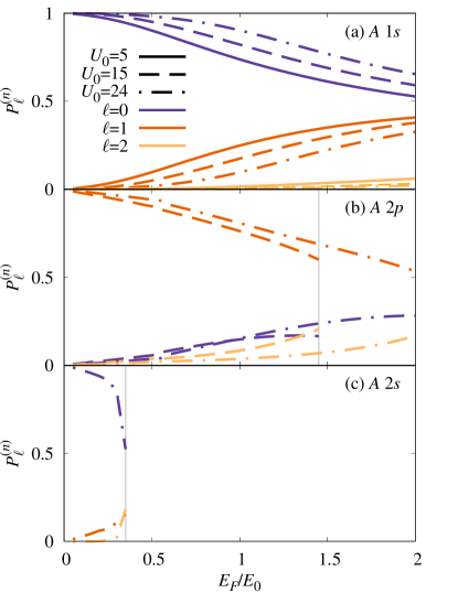
In Fig. 12, we plot the evolution of the probability defined in Eq. (25) as a function of for those eigenvalues that correspond to the , , and attractive branches, for the three different values of that correspond to Figs. 6, 8, and 10, respectively. We see that the attractive branch orbital character is predominantly -wave at low density, as expected, before becoming more -wave with increasing . However, for the attractive branch, even though the -wave character dominates over the entire interval studied, there is an exchange with both - and -wave components when increases. Finally, the attractive branch quickly loses its -wave character towards both the - and -wave components, before merging with the continuum at . We can in general see that, as increases, the exchange of angular momentum components is slower due to the attractive branches moving further apart in energy.
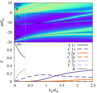
Finally, we note that an alternative way of presenting the polaron spectral properties is one where energy scales are rescaled by and length scales by . In this case, we fix the dipolar interaction parameter (6) and study the polaron spectrum by varying an additional dimensionless parameter, such as or :
We plot in Fig. 13 the impurity spectral function obtained by fixing and increasing . In the units previously employed, this corresponds to simultaneously increasing and decreasing , which we see leads to the binding of an increasing number of dimer states. As shown in Fig. 13(a), the branches with stronger spectral weight are those associated with the -wave dimer states. In panels (b), (c), and (d) of Fig. 13 we plot the spectral function at a fixed value of energy as a function of . As a color map, we plot the fraction of the spectral function with angular momentum , defined as the ratio between the angular momentum weighted spectral function
| (26) |
and — note that . This allows us to identify the dominant orbital angular momentum component of each attractive branch, which we see is strongly correlated with the angular momentum of the corresponding bound dimer state.
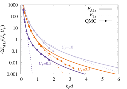
Making use of these units, we compare in Fig. 14 the results for the energy of the attractive branch obtained within the polaron Ansatz (19) with those obtained in Ref. Matveeva and Giorgini (2013) by quantum Monte Carlo (QMC) methods for different values of . For , there is excellent agreement between the two theories for any value of , suggesting that, within this regime, disregarding intralayer interactions is a reliable approximation. For larger values of , perfect agreement is observed only at small values, where the polaron energy closely matches that of the vacuum dimer state. For increasing values, where layer approaches the transition to a broken symmetry phase Parish and Marchetti (2012); Matveeva and Giorgini (2012), we find that deviations increase, although the qualitative behavior remains similar.
V Tunneling rate and impurity spectral function
We now discuss how one can experimentally probe the spectral function. Our proposal is inspired by radiofrequency spectroscopy Punk and Zwerger (2007), where one can inject (eject) the impurity by driving transitions from (to) an auxiliary hyperfine state that, in the ideal case, does not interact with the medium. Similarly, we suggest to use an auxiliary layer () that the impurity can tunnel into/from — see Fig. 15. We furthermore assume that interactions between the dipolar particles can occur only between layers and , while tunneling can only occur between layers and . This situation can, e.g., be achieved if a potential barrier is present between layers and , while layer is further away from both layers. We also note that, in practice, a small 1-3 interaction can be taken into account by considering the initial state to be a weakly dressed attractive polaron, similarly to what is routinely done in the case of RF spectroscopy for contact interactions, see, e.g., Ref. Baym et al. (2007).
We thus have to extend the Hamiltonian (1) to include two additional terms, and , that describe, respectively, the kinetic energy of the particles in layer , and the tunneling between layers 2 and :
| (27a) | ||||
| (27b) | ||||
Note that in the kinetic term we have included a “detuning” energy , which represents the difference between the energy minima of the confining potentials in the -direction.
The additional terms in the Hamiltonian exactly match those used in radiofrequency spectroscopy on impurities Liu et al. (2020), where plays the role of the radiofrequency detuning, and the role of the Rabi coupling. Therefore, this auxiliary layer provides access to the spectral properties. To be specific, within linear response the tunneling rate can be evaluated using Fermi’s golden rule between an initial state consisting of one particle in layer plus a Fermi sea of dipoles in layer , , while the final state is the polaron state (19). This gives
| (28) |
Thus, measuring the tunneling rate as a function of the energy difference between the two lowest eigenenergies of the -confining lattice potentials is equivalent to measuring the polaron spectral function (21b) evaluated in this work.
VI Conclusions and perspectives
In this work we have studied a gas of dipolar fermions in a bilayer geometry in the limit of extreme imbalance, i.e., a single dipole in one layer interacting with a Fermi sea of dipoles in a different layer. We analyze two different yet connected solutions of this problem. We first investigate the properties of the interlayer dimer bound state, generalized to include the Pauli blocking effect from the inert Fermi sea. We find a series of bound states, characterized by the orbital angular momentum and the principal quantum number, binding for increasing dipolar interaction strength or decreasing bilayer distance. For the dimer ground state, we determine the spontaneous emergence of a finite center of mass momentum when increasing above a threshold value. The finite momentum dimer corresponds to the large imbalance limit of the FFLO state studied in Ref. Lee et al. (2017). We find that this state has a mixed partial wave character, including -, -, and -wave contributions.
The other solution we analyze is the many-body polaron state, where the presence of the impurity in one layer leads to particle-hole excitations of the Fermi sea in the other layer. We derive the polaron spectral properties by employing a single particle-hole variational ansatz, and we propose that the tunneling rate of the impurity from an additional auxiliary layer can be employed to experimentally access the spectrum. We find that the polaron spectrum is characterized by a series of attractive polaron branches which we trace back to the dimer bound states. At small , the polaron energies and their orbital character recover those of the dimer states. However, both energies and orbital angular momentum components evolve and interchange with . We find that the energy of the ground-state polaron branch evolves with in a qualitative different way depending on the value of . We explain this distinctive property of finite-range dipole-dipole interactions in terms of whether hole scattering is negligible or not in the polaron formation. We characterize the transfer of oscillator strength from the repulsive branch to the series of attractive branches in terms of their partial wave character and their distance in energy from the repulsive branch.
In our model, we neglect the repulsive interactions between particles in the Fermi sea. As such, we neglect the possibility of strong intralayer correlations that could lead, at very low temperatures, to the spontaneous appearance of density modulated phases such as stripes Parish and Marchetti (2012) and Wigner crystals Matveeva and Giorgini (2012), which are predicted to occur for either strong enough dipolar interactions or large enough Fermi densities. While beyond the scope of our study, an exciting perspective of our work is the generalization of the polaron formalism to include the possibility of the impurity interacting with such strongly correlated phases Matveeva and Giorgini (2013), which could potentially leave signatures in the polaron spectral response. Indeed, this would mirror very recent experiments on exciton polarons in doped 2D semiconductor monolayers which have probed strongly correlated states of 2D electron gases, such as Wigner crystals Smoleński et al. (2021); Shimazaki et al. (2021), fractional quantum Hall states in proximal graphene layers Popert et al. (2022) and correlated-Mott states of electrons in a moiré superlattice Schwartz et al. (2021).
Another interesting perspective of our work would involve considering a configuration where the alignment of the dipoles is tilted at a slight angle relative to the normal direction. In this case, the anisotropy induced by the dipole-dipole interaction results in a distorted Fermi surface Bruun and Taylor (2008); Yamaguchi et al. (2010), consequently influencing the properties of the Fermi polaron and giving rise to spatial anisotropies, as illustrated in a three-dimensional setup by Ref. Nishimura et al. (2021). Indeed, deformations of the Fermi surface have already been experimentally observed in a three-dimensional degenerate dipolar Fermi gas composed of Er atoms Aikawa et al. (2014b). Furthermore, a tilted configuration is expected to stabilize the FFLO state (see, e.g., Ref. Kawamura and Ohashi (2022)) since it breaks the continuous rotational symmetry and thus suppresses the pairing fluctuations that destroy FFLO long-range order Shimahara (1998).
The research data underpinning this publication can be accessed at Ref. Tiene et al. (2024).
Acknowledgements.
We would like to thank Stefano Giorgini for fruitful discussions and for letting us use the data from Ref. Matveeva and Giorgini (2013). AT and FMM acknowledge financial support from the Ministerio de Ciencia e Innovación (MICINN), project No. AEI/10.13039/501100011033 PID2020-113415RB-C22 (2DEnLight). FMM acknowledges financial support from the Proyecto Sinérgico CAM 2020 Y2020/TCS-6545 (NanoQuCo-CM). JL and MMP are supported through Australian Research Council Future Fellowships FT160100244 and FT200100619, respectively. JL and MMP also acknowledge support from the Australian Research Council Centre of Excellence in Future Low-Energy Electronics Technologies (CE170100039).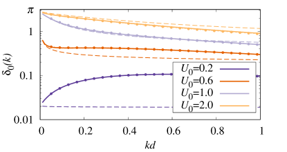
Appendix A Scattering phase shift
In this appendix we evaluate the -wave energy-dependent scattering phase shift , where , with being the reduced mass. We use the variable-phase method Morse and Allis (1933) which allows us to evaluate the phase shift produced by a potential that vanishes for all , i.e., we define . In this sense, the phase shift can be viewed as the accumulated phase shift at position in the true potential . In 2D, satisfies the following first-order, non-linear differential equation Portnoi and Galbraith (1997):
| (29) |
with boundary condition . In this expression, and are Bessel functions of the first and second kinds, respectively (the latter are also called Neumann functions), and is again the orbital angular momentum. Thus, for -wave, . Finally, the scattering phase shift in the true potential is given by the limit , and it is a function of the scattering energy through the momentum in Eq. (29).
The scattering phase shift for the interlayer dipolar potential (2a) has been previously evaluated in Ref. Klawunn et al. (2010b), where the following approximate analytical expression for the -wave scattering phase shift was obtained for small values of :
| (30) |
where , , and
Using Eq. (14), a small- expansion of this expression allows us to recover the universal low-energy expression of the phase shift for a short-range potential with a dimer state with binding energy :
| (31) |
We note that this is the true phase shift for a contact potential; however other potentials will generally have corrections of Levinsen and Parish (2015).
In Fig. 16 we compare the numerical results for the scattering phase shift obtained by solving Eq. (29) with the approximation (30) derived in Ref. Klawunn et al. (2010b) and the universal low-energy expression in Eq. (31). While we see that Eq. (30) is a good approximation for values of , the phase shift for a contact potential is a good approximation only when and . For , as also argued by Ref. Klawunn et al. (2010b), the binding energy of the state becomes anomalously small and thus the expression (31) cannot, in practice, be considered the leading term for the low-energy scattering. However, when , both approximations become increasingly inaccurate since then there are other dimer states that are close to becoming bound.
Appendix B Relation between -matrix approach and the variational ansatz
We now discuss the relationship between the -matrix approach used to obtain the lowest energy attractive polaron branch in Ref. Klawunn and Recati (2013) and the variational ansatz (19) that we employ in this work.
For a finite-range scattering potential , the matrix describes the scattering between an incoming impurity with momentum and a bath fermion with momentum which are exchanging a momentum . By using a diagrammatic expansion within the ladder approximation (see Fig. 17(a)), all terms can be re-summed to give an implicit equation for the matrix. Considering, for simplicity, the case of an impurity with zero momentum , one obtains the following implicit equation for the matrix:
| (32) |
Here, is the Fermi-Dirac distribution, i.e., at zero temperature , and is the initial energy of the scattering process.

Starting from the matrix, one can evaluate the entire polaron spectrum by evaluating the impurity Green’s function in terms of the self-energy — see Fig. 17(b):
| (33a) | ||||
| (33b) | ||||
The spectral function is then obtained from the Green’s function as in Eq. (21b).
The matrix can also be obtained directly from the polaron eigenvalue equations (20). Defining
| (34) |
Eq. (20b) becomes
| (35) |
If one neglects the last term, this equation coincides with Eq. (32) by changing variable and redefining
| (36) |
The last term in Eq. (35) describes the scattering of the impurity with a hole of the fermionic bath and corresponds to the term in the polaron eigenvalue equations (20). For a contact interaction potential, the terms can be safely neglected Chevy (2006) because the phase space for hole scattering is small. However, this is not always true for a longer-range potential such as the interlayer dipolar potential.
In order to show this, we plot in Fig. 18 the lowest polaron energy as well as the entire polaron spectrum, comparing the results of three methods: (1) by solving the polaron eigenvalue problem (20), (2) by neglecting the term in Eq. (20), and (3) by numerically solving the -matrix equation (32) (see below). Methods (2) and (3) give exactly the same results, as they should. However, there is a non-negligible shift compared with the results obtained with method (1) if either is large, , or if . This coincides with the regime where the interlayer dipolar potential gives a very different scattering phase shift to that of the contact potential — see App. A. In particular, the solution of the full problem without neglecting the term is always blueshifted in energy compared to the case where one neglects the scattering of the impurity with the holes in the Fermi sea. This shift increases both as a function of and . If is large, , as in Fig. 18, then the overall redshift of the attractive polaron branch as a function of can be changed into a blueshift.
To numerically solve for the matrix, we can assume that it depends only on a single angle, the one between and (-wave ansatz), so that the implicit equation (32) can be easily solved by direct inversion. If we define vector indices by and , the matrix becomes
where , and the matrix kernel is
Similarly, Eq. (35) can also be solved by inversion, with the difference that now the vector space has a larger dimension. If we define the vector index as , where is the angle between and , and if we use the notation and , we find that the matrix can be evaluated as
| (37) |
where , and where the two kernels are
The variational ansatz thus allows repeated impurity-hole scattering, unlike the -matrix formulation. Note that this is qualitatively different from screening effects such as the Gork’ov–Melik-Barkhudarov particle-hole screening of the particle-particle correlations responsible for superfluidity in the Bose-Einstein-condensate-Bardeen-Cooper-Schrieffer (BEC-BCS) crossover Pisani et al. (2018). In particular, an additional excitation would be required to screen the interactions between the impurity and a fermion from the medium. This would be an interesting future direction of research, but is beyond the scope of the current work.
References
- Lahaye et al. (2009) T. Lahaye, C. Menotti, L. Santos, M. Lewenstein, and T. Pfau, The physics of dipolar bosonic quantum gases, Rep. Prog. Phys. 72, 126401 (2009).
- Baranov et al. (2012) M. A. Baranov, M. Dalmonte, G. Pupillo, and P. Zoller, Condensed Matter Theory of Dipolar Quantum Gases, Chem. Rev. 112, 5012 (2012).
- Chomaz et al. (2022) L. Chomaz, I. Ferrier-Barbut, F. Ferlaino, B. Laburthe-Tolra, B. L. Lev, and T. Pfau, Dipolar physics: a review of experiments with magnetic quantum gases, Rep. Prog. Phys. 86, 026401 (2022).
- Griesmaier et al. (2005) A. Griesmaier, J. Werner, S. Hensler, J. Stuhler, and T. Pfau, Bose-Einstein Condensation of Chromium, Phys. Rev. Lett. 94, 160401 (2005).
- Stuhler et al. (2005) J. Stuhler, A. Griesmaier, T. Koch, M. Fattori, T. Pfau, S. Giovanazzi, P. Pedri, and L. Santos, Observation of Dipole-Dipole Interaction in a Degenerate Quantum Gas, Phys. Rev. Lett. 95, 150406 (2005).
- Lu et al. (2011) M. Lu, N. Q. Burdick, S. H. Youn, and B. L. Lev, Strongly Dipolar Bose-Einstein Condensate of Dysprosium, Phys. Rev. Lett. 107, 190401 (2011).
- Lu et al. (2012) M. Lu, N. Q. Burdick, and B. L. Lev, Quantum Degenerate Dipolar Fermi Gas, Phys. Rev. Lett. 108, 215301 (2012).
- Aikawa et al. (2012) K. Aikawa, A. Frisch, M. Mark, S. Baier, A. Rietzler, R. Grimm, and F. Ferlaino, Bose-Einstein Condensation of Erbium, Phys. Rev. Lett. 108, 210401 (2012).
- Aikawa et al. (2014a) K. Aikawa, A. Frisch, M. Mark, S. Baier, R. Grimm, J. L. Bohn, D. S. Jin, G. M. Bruun, and F. Ferlaino, Anisotropic Relaxation Dynamics in a Dipolar Fermi Gas Driven Out of Equilibrium, Phys. Rev. Lett. 113, 263201 (2014a).
- Böttcher et al. (2020) F. Böttcher, J.-N. Schmidt, J. Hertkorn, K. S. H. Ng, S. D. Graham, M. Guo, T. Langen, and T. Pfau, New states of matter with fine-tuned interactions: quantum droplets and dipolar supersolids, Rep. Prog. Phys. 84, 012403 (2020).
- Löw et al. (2012) R. Löw, H. Weimer, J. Nipper, J. B. Balewski, B. Butscher, H. P. Büchler, and T. Pfau, An experimental and theoretical guide to strongly interacting Rydberg gases, Journal of Physics B: Atomic, Molecular and Optical Physics 45, 113001 (2012).
- Moses et al. (2017) S. Moses, J. Covey, M. Miecnikowski, D. Jin, and J. Ye, New frontiers for quantum gases of polar molecules, Nature Physics 13, 13 (2017).
- Shaffer et al. (2018) J. P. Shaffer, S. T. Rittenhouse, and H. R. Sadeghpour, Ultracold Rydberg molecules, Nature Communications 9, 1965 (2018).
- Valtolina et al. (2020) G. Valtolina, K. Matsuda, W. G. Tobias, J.-R. Li, L. De Marco, and J. Ye, Dipolar evaporation of reactive molecules to below the Fermi temperature, Nature 588, 239 (2020).
- Marco et al. (2019) L. D. Marco, G. Valtolina, K. Matsuda, W. G. Tobias, J. P. Covey, and J. Ye, A degenerate Fermi gas of polar molecules, Science 363, 853 (2019).
- Tobias et al. (2020) W. G. Tobias, K. Matsuda, G. Valtolina, L. De Marco, J.-R. Li, and J. Ye, Thermalization and Sub-Poissonian Density Fluctuations in a Degenerate Molecular Fermi Gas, Phys. Rev. Lett. 124, 033401 (2020).
- Schindewolf et al. (2022) A. Schindewolf, R. Bause, X.-Y. Chen, M. Duda, T. Karman, I. Bloch, and X.-Y. Luo, Evaporation of microwave-shielded polar molecules to quantum degeneracy, Nature 607, 677 (2022).
- Duda et al. (2023) M. Duda, X.-Y. Chen, A. Schindewolf, R. Bause, J. von Milczewski, R. Schmidt, I. Bloch, and X.-Y. Luo, Transition from a polaronic condensate to a degenerate Fermi gas of heteronuclear molecules, Nature Physics 19, 720 (2023).
- Deiglmayr et al. (2008) J. Deiglmayr, A. Grochola, M. Repp, K. Mörtlbauer, C. Glück, J. Lange, O. Dulieu, R. Wester, and M. Weidemüller, Formation of Ultracold Polar Molecules in the Rovibrational Ground State, Phys. Rev. Lett. 101, 133004 (2008).
- Repp et al. (2013) M. Repp, R. Pires, J. Ulmanis, R. Heck, E. D. Kuhnle, M. Weidemüller, and E. Tiemann, Observation of interspecies 6Li-133Cs Feshbach resonances, Phys. Rev. A 87, 010701 (2013).
- Park et al. (2023) J. J. Park, Y.-K. Lu, A. O. Jamison, T. V. Tscherbul, and W. Ketterle, A Feshbach resonance in collisions between triplet ground-state molecules, Nature 614, 54 (2023).
- Tobias et al. (2022) W. G. Tobias, K. Matsuda, J.-R. Li, C. Miller, A. N. Carroll, T. Bilitewski, A. M. Rey, and J. Ye, Reactions between layer-resolved molecules mediated by dipolar spin exchange, Science 375, 1299 (2022).
- Cooper and Shlyapnikov (2009) N. R. Cooper and G. V. Shlyapnikov, Stable Topological Superfluid Phase of Ultracold Polar Fermionic Molecules, Phys. Rev. Lett. 103, 155302 (2009).
- Levinsen et al. (2011) J. Levinsen, N. R. Cooper, and G. V. Shlyapnikov, Topological superfluid phase of fermionic polar molecules, Phys. Rev. A 84, 013603 (2011).
- Bruun and Taylor (2008) G. M. Bruun and E. Taylor, Quantum Phases of a Two-Dimensional Dipolar Fermi Gas, Phys. Rev. Lett. 101, 245301 (2008).
- Yamaguchi et al. (2010) Y. Yamaguchi, T. Sogo, T. Ito, and T. Miyakawa, Density-wave instability in a two-dimensional dipolar Fermi gas, Phys. Rev. A 82, 013643 (2010).
- Sun et al. (2010) K. Sun, C. Wu, and S. Das Sarma, Spontaneous inhomogeneous phases in ultracold dipolar Fermi gases, Phys. Rev. B 82, 075105 (2010).
- Parish and Marchetti (2012) M. M. Parish and F. M. Marchetti, Density Instabilities in a Two-Dimensional Dipolar Fermi Gas, Phys. Rev. Lett. 108, 145304 (2012).
- Matveeva and Giorgini (2012) N. Matveeva and S. Giorgini, Liquid and Crystal Phases of Dipolar Fermions in Two Dimensions, Phys. Rev. Lett. 109, 200401 (2012).
- Marchetti and Parish (2013) F. M. Marchetti and M. M. Parish, Density-wave phases of dipolar fermions in a bilayer, Phys. Rev. B 87, 045110 (2013).
- Klawunn et al. (2010a) M. Klawunn, J. Duhme, and L. Santos, Bose-Fermi mixtures of self-assembled filaments of fermionic polar molecules, Phys. Rev. A 81, 013604 (2010a).
- Potter et al. (2010) A. C. Potter, E. Berg, D.-W. Wang, B. I. Halperin, and E. Demler, Superfluidity and Dimerization in a Multilayered System of Fermionic Polar Molecules, Phys. Rev. Lett. 105, 220406 (2010).
- Pikovski et al. (2010) A. Pikovski, M. Klawunn, G. V. Shlyapnikov, and L. Santos, Interlayer Superfluidity in Bilayer Systems of Fermionic Polar Molecules, Phys. Rev. Lett. 105, 215302 (2010).
- Klawunn et al. (2010b) M. Klawunn, A. Pikovski, and L. Santos, Two-dimensional scattering and bound states of polar molecules in bilayers, Phys. Rev. A 82, 044701 (2010b).
- Mazloom and Abedinpour (2018) A. Mazloom and S. H. Abedinpour, Interplay of interlayer pairing and many-body screening in a bilayer of dipolar fermions, Phys. Rev. B 98, 014513 (2018).
- Mazloom and Abedinpour (2017) A. Mazloom and S. H. Abedinpour, Superfluidity in density imbalanced bilayers of dipolar fermions, Phys. Rev. B 96, 064513 (2017).
- Lee et al. (2017) H. Lee, S. I. Matveenko, D.-W. Wang, and G. V. Shlyapnikov, Fulde-Ferrell-Larkin-Ovchinnikov state in bilayer dipolar systems, Phys. Rev. A 96, 061602 (2017).
- Klawunn and Recati (2013) M. Klawunn and A. Recati, Polar molecules in bilayers with high population imbalance, Phys. Rev. A 88, 013633 (2013).
- Matveeva and Giorgini (2013) N. Matveeva and S. Giorgini, Impurity Problem in a Bilayer System of Dipoles, Phys. Rev. Lett. 111, 220405 (2013).
- Note (1) The “repulsive Fermi polaron” problem with dipolar fermions in a single layer geometry has been considered in Ref. Bombín et al. (2019).
- Zöllner et al. (2011) S. Zöllner, G. M. Bruun, and C. J. Pethick, Polarons and molecules in a two-dimensional Fermi gas, Phys. Rev. A 83, 021603 (2011).
- Parish (2011) M. M. Parish, Polaron-molecule transitions in a two-dimensional Fermi gas, Phys. Rev. A 83, 051603 (2011).
- Schmidt et al. (2012a) R. Schmidt, T. Enss, V. Pietilä, and E. Demler, Fermi polarons in two dimensions, Phys. Rev. A 85, 021602 (2012a).
- Ngampruetikorn et al. (2012) V. Ngampruetikorn, J. Levinsen, and M. M. Parish, Repulsive polarons in two-dimensional Fermi gases, Europhysics Letters 98, 30005 (2012).
- Parish and Levinsen (2013) M. M. Parish and J. Levinsen, Highly polarized Fermi gases in two dimensions, Phys. Rev. A 87, 033616 (2013).
- Tajima et al. (2021) H. Tajima, J. Takahashi, S. I. Mistakidis, E. Nakano, and K. Iida, Polaron Problems in Ultracold Atoms: Role of a Fermi Sea across Different Spatial Dimensions and Quantum Fluctuations of a Bose Medium, Atoms 9, 18 (2021).
- Sidler et al. (2016) M. Sidler, P. Back, O. Cotlet, A. Srivastava, T. Fink, M. Kroner, E. Demler, and A. Imamoglu, Fermi polaron-polaritons in charge-tunable atomically thin semiconductors, Nature Physics 13, 255 (2016).
- Efimkin et al. (2021) D. K. Efimkin, E. K. Laird, J. Levinsen, M. M. Parish, and A. H. MacDonald, Electron-exciton interactions in the exciton-polaron problem, Phys. Rev. B 103, 075417 (2021).
- Tiene et al. (2022) A. Tiene, J. Levinsen, J. Keeling, M. M. Parish, and F. M. Marchetti, Effect of fermion indistinguishability on optical absorption of doped two-dimensional semiconductors, Phys. Rev. B 105, 125404 (2022).
- Huang et al. (2023) D. Huang, K. Sampson, Y. Ni, Z. Liu, D. Liang, K. Watanabe, T. Taniguchi, H. Li, E. Martin, J. Levinsen, M. M. Parish, E. Tutuc, D. K. Efimkin, and X. Li, Quantum Dynamics of Attractive and Repulsive Polarons in a Doped Monolayer, Phys. Rev. X 13, 011029 (2023).
- Yang et al. (1991) X. L. Yang, S. H. Guo, F. T. Chan, K. W. Wong, and W. Y. Ching, Analytic solution of a two-dimensional hydrogen atom. I. Nonrelativistic theory, Phys. Rev. A 43, 1186 (1991).
- Massignan et al. (2014) P. Massignan, M. Zaccanti, and G. M. Bruun, Polarons, dressed molecules and itinerant ferromagnetism in ultracold Fermi gases, Rep. Prog. Phys. 77, 034401 (2014).
- Scazza et al. (2022) F. Scazza, M. Zaccanti, P. Massignan, M. M. Parish, and J. Levinsen, Repulsive Fermi and Bose Polarons in Quantum Gases, Atoms 10, 55 (2022).
- Li et al. (2010) Q. Li, E. H. Hwang, and S. Das Sarma, Collective modes of monolayer, bilayer, and multilayer fermionic dipolar liquid, Phys. Rev. B 82, 235126 (2010).
- Note (2) Note that Refs. Lahaye et al. (2009); Chomaz et al. (2022) use a different definition of but the same definition of : .
- Du et al. (2023) L. Du, P. Barral, M. Cantara, J. de Hond, Y.-K. Lu, and W. Ketterle, Atomic physics on a 50 nm scale: Realization of a bilayer system of dipolar atoms (2023), arXiv:2302.07209 [cond-mat.quant-gas] .
- Carr et al. (2009) L. D. Carr, D. DeMille, R. V. Krems, and J. Ye, Cold and ultracold molecules: science, technology and applications, New Journal of Physics 11, 055049 (2009).
- Note (3) Note that, as mentioned previously, the Schrödinger equation becomes diagonal in when either or , such that symmetric and antisymmetric solutions become degenerate.
- Yudson et al. (1997) V. I. Yudson, M. G. Rozman, and P. Reineker, Bound states of two particles confined to parallel two-dimensional layers and interacting via dipole-dipole or dipole-charge laws, Phys. Rev. B 55, 5214 (1997).
- Parish et al. (2011) M. M. Parish, F. M. Marchetti, and P. B. Littlewood, Supersolidity in electron-hole bilayers with a large density imbalance, Europhysics Letters 95, 27007 (2011).
- Cotlet et al. (2020) O. Cotlet, D. S. Wild, M. D. Lukin, and A. Imamoglu, Rotons in optical excitation spectra of monolayer semiconductors, Phys. Rev. B 101, 205409 (2020).
- Tiene et al. (2020) A. Tiene, J. Levinsen, M. M. Parish, A. H. MacDonald, J. Keeling, and F. M. Marchetti, Extremely imbalanced two-dimensional electron-hole-photon systems, Phys. Rev. Res. 2, 023089 (2020).
- Fulde and Ferrell (1964) P. Fulde and R. A. Ferrell, Superconductivity in a Strong Spin-Exchange Field, Phys. Rev. 135, A550 (1964).
- Larkin and Ovchinnikov (1964) A. I. Larkin and Y. N. Ovchinnikov, Nonuniform state of superconductors, Zh. Eksp. Teor. Fiz. 47, 1136 (1964).
- Casalbuoni and Nardulli (2004) R. Casalbuoni and G. Nardulli, Inhomogeneous superconductivity in condensed matter and QCD, Rev. Mod. Phys. 76, 263 (2004).
- Radzihovsky and Sheehy (2010) L. Radzihovsky and D. E. Sheehy, Imbalanced Feshbach-resonant Fermi gases, Rep. Prog. Phys. 73, 076501 (2010).
- Chevy (2006) F. Chevy, Universal phase diagram of a strongly interacting Fermi gas with unbalanced spin populations, Phys. Rev. A 74, 063628 (2006).
- Combescot and Giraud (2008) R. Combescot and S. Giraud, Normal State of Highly Polarized Fermi Gases: Full Many-Body Treatment, Phys. Rev. Lett. 101, 050404 (2008).
- Combescot et al. (2007) R. Combescot, A. Recati, C. Lobo, and F. Chevy, Normal State of Highly Polarized Fermi Gases: Simple Many-Body Approaches, Phys. Rev. Lett. 98, 180402 (2007).
- Baranov et al. (2011) M. A. Baranov, A. Micheli, S. Ronen, and P. Zoller, Bilayer superfluidity of fermionic polar molecules: Many-body effects, Phys. Rev. A 83, 043602 (2011).
- Mahan (2000) G. Mahan, Many-Particle Physics (Kluwer Academic/Plenum Publishers, 2000).
- Note (4) Note that we only plot the dimer energy at finite center of mass corresponding to the symmetric states under the exchange in Eq. (12\@@italiccorr) since these are the only ones with finite spectral weight. Instead, for zero center of mass momentum, symmetric and antisymmetric solution are degenerate in energy.
- Schmidt et al. (2012b) R. Schmidt, T. Enss, V. Pietilä, and E. Demler, Fermi polarons in two dimensions, Phys. Rev. A 85 (2012b).
- Note (5) Note that only for the state do we always have .
- Punk and Zwerger (2007) M. Punk and W. Zwerger, Theory of rf-Spectroscopy of Strongly Interacting Fermions, Phys. Rev. Lett. 99, 170404 (2007).
- Baym et al. (2007) G. Baym, C. J. Pethick, Z. Yu, and M. W. Zwierlein, Coherence and Clock Shifts in Ultracold Fermi Gases with Resonant Interactions, Phys. Rev. Lett. 99, 190407 (2007).
- Liu et al. (2020) W. E. Liu, Z.-Y. Shi, M. M. Parish, and J. Levinsen, Theory of radio-frequency spectroscopy of impurities in quantum gases, Phys. Rev. A 102, 023304 (2020).
- Smoleński et al. (2021) T. Smoleński, P. E. Dolgirev, C. Kuhlenkamp, A. Popert, Y. Shimazaki, P. Back, X. Lu, M. Kroner, K. Watanabe, T. Taniguchi, I. Esterlis, E. Demler, and A. Imamoğlu, Signatures of Wigner crystal of electrons in a monolayer semiconductor, Nature 595, 53 (2021).
- Shimazaki et al. (2021) Y. Shimazaki, C. Kuhlenkamp, I. Schwartz, T. Smoleński, K. Watanabe, T. Taniguchi, M. Kroner, R. Schmidt, M. Knap, and A. Imamoğlu, Optical Signatures of Periodic Charge Distribution in a Mott-like Correlated Insulator State, Phys. Rev. X 11, 021027 (2021).
- Popert et al. (2022) A. Popert, Y. Shimazaki, M. Kroner, K. Watanabe, T. Taniguchi, A. Imamoğlu, and T. Smoleński, Optical Sensing of Fractional Quantum Hall Effect in Graphene, Nano Letters 22, 7363 (2022).
- Schwartz et al. (2021) I. Schwartz, Y. Shimazaki, C. Kuhlenkamp, K. Watanabe, T. Taniguchi, M. Kroner, and A. Imamoğlu, Electrically tunable Feshbach resonances in twisted bilayer semiconductors, Science 374, 336 (2021).
- Nishimura et al. (2021) K. Nishimura, E. Nakano, K. Iida, H. Tajima, T. Miyakawa, and H. Yabu, Ground state of the polaron in an ultracold dipolar Fermi gas, Phys. Rev. A 103, 033324 (2021).
- Aikawa et al. (2014b) K. Aikawa, S. Baier, A. Frisch, M. Mark, C. Ravensbergen, and F. Ferlaino, Observation of Fermi surface deformation in a dipolar quantum gas, Science 345, 1484 (2014b).
- Kawamura and Ohashi (2022) T. Kawamura and Y. Ohashi, Feasibility of a Fulde-Ferrell-Larkin-Ovchinnikov superfluid Fermi atomic gas, Phys. Rev. A 106, 033320 (2022).
- Shimahara (1998) H. Shimahara, Phase Fluctuations and Kosterlitz-Thouless Transition in Two-Dimensional Fulde-Ferrell-Larkin-Ovchinnikov Superconductors, Journal of the Physical Society of Japan 67, 1872 (1998).
- Tiene et al. (2024) A. Tiene, A. Tamargo Bracho, M. M. Parish, J. Levinsen, and F. M. Marchetti, Multiple polaron quasiparticles with dipolar fermions in a bilayer geometry (dataset) (2024).
- Morse and Allis (1933) P. M. Morse and W. P. Allis, The Effect of Exchange on the Scattering of Slow Electrons from Atoms, Phys. Rev. 44, 269 (1933).
- Portnoi and Galbraith (1997) M. Portnoi and I. Galbraith, Variable-phase method and Levinson’s theorem in two dimensions: Application to a screened Coulomb potential, Solid State Communications 103, 325 (1997).
- Levinsen and Parish (2015) J. Levinsen and M. M. Parish, Strongly interacting two-dimensional Fermi gases, Annual Review of Cold Atoms and Molecules 3, 1 (2015).
- Pisani et al. (2018) L. Pisani, A. Perali, P. Pieri, and G. C. Strinati, Entanglement between pairing and screening in the Gorkov-Melik-Barkhudarov correction to the critical temperature throughout the BCS-BEC crossover, Phys. Rev. B 97, 014528 (2018).
- Bombín et al. (2019) R. Bombín, T. Comparin, G. Bertaina, F. Mazzanti, S. Giorgini, and J. Boronat, Two-dimensional repulsive Fermi polarons with short- and long-range interactions, Phys. Rev. A 100, 023608 (2019).