Multiple-GPU accelerated high-order gas-kinetic scheme for direct numerical simulation of compressible turbulence
Abstract
High-order gas-kinetic scheme (HGKS) has become a workable tool for the direct numerical simulation (DNS) of turbulence. In this paper, to accelerate the computation, HGKS is implemented with the graphical processing unit (GPU) using the compute unified device architecture (CUDA). Due to the limited available memory size, the computational scale is constrained by single GPU. To conduct the much large-scale DNS of turbulence, HGKS also be further upgraded with multiple GPUs using message passing interface (MPI) and CUDA architecture. The benchmark cases for compressible turbulence, including Taylor-Green vortex and turbulent channel flows, are presented to assess the numerical performance of HGKS with Nvidia TITAN RTX and Tesla V100 GPUs. For single-GPU computation, compared with the parallel central processing unit (CPU) code running on the Intel Core i7-9700 with open multi-processing (OpenMP) directives, 7x speedup is achieved by TITAN RTX and 16x speedup is achieved by Tesla V100. For multiple-GPU computation, multiple-GPU accelerated HGKS code scales properly with the increasing number of GPU. The computational time of parallel CPU code running on Intel Xeon E5-2692 cores with MPI is approximately times longer than that of GPU code using Tesla V100 GPUs with MPI and CUDA. Numerical results confirm the excellent performance of multiple-GPU accelerated HGKS for large-scale DNS of turbulence. Alongside the footprint in reduction of loading and writing pressure of GPU memory, HGKS in GPU is also compiled with FP32 precision to evaluate the effect of number formats precision. Reasonably, compared to the computation with FP64 precision, the efficiency is improved and the memory cost is reduced with FP32 precision. Meanwhile, the differences in accuracy for statistical turbulent quantities appear. For turbulent channel flows, difference in long-time statistical turbulent quantities is acceptable between FP32 and FP64 precision solutions. While the obvious discrepancy in instantaneous turbulent quantities can be observed, which shows that FP32 precision is not safe for DNS in compressible turbulence. The choice of precision should depended on the requirement of accuracy and the available computational resources.
keywords:
High-order gas-kinetic scheme, direct numerical simulation, compressible turbulence, multiple-GPU accelerated computation.1 Introduction
Turbulence is ubiquitous in natural phenomena and engineering applications [1]. The understanding and prediction of multiscale turbulent flow is one of the most difficult problems for both mathematics and physical sciences. Direct numerical simulation (DNS) solves the Navier-Stokes equations directly, resolve all scales of the turbulent motion, and eliminate modeling entirely [2]. With the advances of high-order numerical methods and supercomputers, great success has been achieved for the incompressible and compressible turbulent flow, such as DNS in incompressible isotropic turbulence [3], incompressible turbulent channel flow [4, 5], supersonic isotropic turbulence [6, 7], compressible turbulent channel flows [8, 9, 10], and compressible flat plate turbulence from the supersonic to hypersonic regime [11, 12].
In the past decades, the gas-kinetic scheme (GKS) has been developed systematically based on the Bhatnagar-Gross-Krook (BGK) model [13, 14] under the finite volume framework, and applied successfully in the computations from low speed flow to hypersonic one [15, 16]. The gas-kinetic scheme presents a gas evolution process from kinetic scale to hydrodynamic scale, where both inviscid and viscous fluxes are recovered from a time-dependent and genuinely multi-dimensional gas distribution function at a cell interface. Starting from a time-dependent flux function, based on the two-stage fourth-order formulation [17, 18], the high-order gas-kinetic scheme (HGKS) has been constructed and applied for the compressible flow simulation [7, 19, 20, 21]. The high-order can be achieved with the implementation of the traditional second-order GKS flux solver. More importantly, the high-order GKS is as robust as the second-order scheme and works perfectly from the subsonic to hypersonic viscous heat conducting flows. Originally, the parallel HGKS code was developed with central processing unit (CPU) using open multi-processing (OpenMP) directives. However, due to the limited shared memory, the computational scale is constrained for numerical simulation of turbulence. To perform the large-scale DNS, the domain decomposition and the message passing interface (MPI) [22] are used for parallel implementation [23]. Due to the explicit formulation of HGKS, the CPU code with MPI scales properly with the number of processors used. The numerical results demonstrates the capability of HGKS as a powerful DNS tool from the low speed to supersonic turbulence study [23].
Graphical processing unit (GPU) is a form of hardware acceleration, which is originally developed for graphics manipulation and is extremely efficient at processing large amounts of data in parallel. Since these units have a parallel computation capability inherently, they can provide fast and low cost solutions to high performance computing (HPC). In recent years, GPUs have gained significant popularity in computational fluid dynamics [24, 25, 26] as a cheaper, more efficient, and more accessible alternative to large-scale HPC systems with CPUs. Especially, to numerically study the turbulent physics in much higher Reynolds number turbulence, the extreme-scale DNS in turbulent flows has been implemented using multiple GPUs, i.e., incompressible isotropic turbulence up to resolution [27] and turbulent pipe flow up to [28]. Recently, the three-dimension discontinuous Galerkin based HGKS has been implemented in single-GPU computation using compute unified device architecture (CUDA) [29]. Obtained results are compared with those obtained by Intel i7-9700 CPU using OpenMP directives. The GPU code achieves 6x-7x speedup with TITAN RTX, and 10x-11x speedup with Tesla V100. The numerical results confirm the potential of HGKS for large-scale DNS in turbulence.
A major limitation in single-GPU computation is its available memory, which leads to a bottleneck in the maximum number of computational mesh. In this paper, to implement much larger scale DNS and accelerate the efficiency, HGKS is implemented with multiple GPUs using CUDA and MPI architecture (MPI + CUDA). It is not straightforward for the multiple-GPU programming, since the memory is not shared across the GPUs and their tasks need to be coordinated appropriately. The multiple GPUs are distributed across multiple CPUs at the cost of having to coordinate GPU-GPU communication via MPI. For WENO-based HGKS in single-GPU using CUDA, compared with the CPU code using Intel Core i7-9700, 7x speedup is achieved for TITAN RTX and 16x speedup is achieved for Tesla V100. In terms of the computation with multiple GPUs, the HGKS code scales properly with the increasing number of GPU. Numerical performance shows that the data communication crossing GPU through MPI costs the relative little time, while the computation time for flow field is the dominant one in the HGKS code. For the MPI parallel computation, the computational time of CPU code with supercomputer using 1024 Intel Xeon E5-2692 cores is approximately times longer than that of GPU code using Tesla V100 GPUs. It can be inferred that the efficiency of GPU code with Tesla V100 GPUs approximately equals to that of MPI code using CPU cores in supercomputer. To reduce the loading and writing pressure of GPU memory, the benefits can be achieved by using FP32 (single) precision compared with FP64 (double) precision for memory-intensive computing [30, 31]. Thence, HGKS in GPUs is compiled with both FP32 precision and FP64 precision to evaluate the effect of precision on DNS of compressible turbulence. As expect, the efficiency can be improved and the memory cost can be reduced with FP32 precision. However, the difference in accuracy between FP32 and FP64 precision appears for the instantaneous statistical quantities of turbulent channel flows, which is not negligible for long time simulations.
This paper is organized as follows. In Section 2, the high-order gas-kinetic scheme is briefly reviewed. The GPU architecture and code design are introduced in Section 3. Section 4 includes numerical simulation and discussions. The last section is the conclusion.
2 High-order gas-kinetic scheme
The three-dimensional BGK equation [13, 14] can be written as
| (1) |
where is the particle velocity, is the gas distribution function, is the three-dimensional Maxwellian distribution and is the collision time. The collision term satisfies the compatibility condition
| (2) |
where , , , is the internal degree of freedom, is the specific heat ratio and is used in the computation.
In this section, the finite volume scheme on orthogonal structured mesh is provided as example. Taking moments of the BGK equation Eq.(1) and integrating with respect to the cell , the finite volume scheme can be expressed as
| (3) |
where is the cell averaged conservative variable over , and the operator reads
| (4) |
where is defined as with , and is the numerical flux across the cell interface . The numerical flux in -direction is given as example
where is the outer normal direction. The Gaussian quadrature is used over the cell interface, where is the quadrature weight, and is the Gauss quadrature point of cell interface . Based on the integral solution of BGK equation Eq.(1), the gas distribution function in the local coordinate can be given by
| (5) |
where is the trajectory of particles, is the initial gas distribution function, and is the corresponding equilibrium state. With the first order spatial derivatives, the second-order gas distribution function at cell interface can be expressed as
| (6) |
where the equilibrium state and the corresponding conservative variables can be determined by the compatibility condition
The following numerical tests on the compressible turbulent flows without discontinuities will be presented, thus the collision time for the flow without discontinuities takes
where is viscous coefficient and is the pressure at cell interface determined by . With the reconstruction of macroscopic variables, the coefficients in Eq.(2) can be fully determined by the reconstructed derivatives and compatibility condition
where and are the moments of the equilibrium and defined by
More details of the gas-kinetic scheme can be found in the literature [15, 16]. Thus, the numerical flux can be obtained by taking moments of the gas distribution function Eq.(2), and the semi-discretized finite volume scheme Eq.(3) can be fully given.
Recently, based on the time-dependent flux function of the generalized Riemann problem solver (GRP) [17, 18] and gas-kinetic scheme [19, 20, 21], a two-stage fourth-order time-accurate discretization was recently developed for Lax-Wendroff type flow solvers. A reliable framework was provided to construct higher-order gas-kinetic scheme, and the high-order scheme is as robust as the second-order one and works perfectly from the subsonic to hypersonic flows. In this study, the two-stage method is used for temporal accuracy. Consider the following time dependent equation
with the initial condition at , i.e., , where is an operator for spatial derivative of flux, the state at can be updated with the following formula
| (7) |
It can be proved that for hyperbolic equations the above temporal discretization Eq.(7) provides a fourth-order time accurate solution for . To implement two-stage fourth-order method for Eq.(3), a linear function is used to approximate the time dependent numerical flux
| (8) |
Integrating Eq.(8) over and , we have the following two equations
The coefficients and at the initial stage can be determined by solving the linear system. According to Eq.(4), and the temporal derivative at can be constructed by
The flow variables at the intermediate stage can be updated. Similarly, , at the intermediate state can be constructed and can be updated as well. For the high-order spatial accuracy, the fifth-order WENO method [32, 33] is adopted. For the three-dimensional computation, the dimension-by-dimension reconstruction is used for HGKS [20].
3 HGKS code design on GPU
CPUs and GPUs are equipped with different architectures and are built for different purposes. The CPU is suited to general workloads, especially those for which per-core performance are important. CPU is designed to execute complex logical tasks quickly, but is limited in the number of threads. Meanwhile, GPU is a form of hardware acceleration, which is originally developed for graphics manipulation and is extremely efficient at processing large amounts of data in parallel. Currently, GPU has gained significant popularity in high performance scientific computing [24, 25, 26]. In this paper, to accelerate the computation, the WENO based HGKS will be implemented with single GPU using CUDA. To conduct the large-scale DNS in turbulence efficiently, the HGKS also be further upgraded with multiple GPUs using MPI + CUDA.
3.1 Single-GPU accelerated HGKS
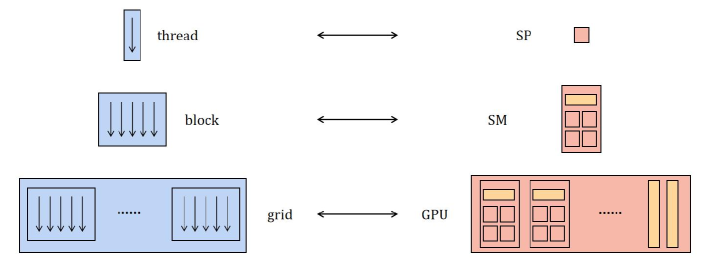
The CPU is regarded as host, and GPU is treated as device. Data-parallel, compute-intensive operations running on the host are transferred to device by using kernels, and kernels are executed on the device by many different threads. For CUDA, these threads are organized into thread blocks, and thread blocks constitute a grid. Such computational structures build connection with Nvidia GPU hardware architecture. The Nvidia GPU consists of multiple streaming multiprocessors (SMs), and each SM contains streaming processors (SPs). When invoking a kernel, the blocks of grid are distributed to SMs, and the threads of each block are executed by SPs. In summary, the correspondence between software CUDA and hardware Nvidia GPU is simply shown in Fig.1. In the following, the single-GPU accelerated HGKS will be introduced briefly.
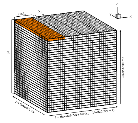
Device implementation is handled automatically by the CUDA, while the kernels and grids need to be specified for HGKS. One updating step of single-GPU accelerated HGKS code can be divided into several kernels, namely, initialization, calculation of time step, WENO reconstruction, flux computation at cell interface in , , , and the update of flow variables. The main parts of the single-GPU accelerated HGKS code are labeled in blue as Algorithm.1. Due to the identical processes of calculation for each kernel, it is natural to use one thread for one computational cell when setting grids. Due to the limited number of threads can be obtained in one block (i.e., the maximum threads in one block), the whole computational domain is required to be divided into several parts. Assume that the total number of cells for computational mesh is , which is illustrated in Fig.2. The computational domain is divided into parts in -direction, where the choice of for each kernel is an integer defined according to the requirement and experience. If is not divisible by , an extra block is needed. When setting grid, the variables ”dimGrid” and ”dimBlock” are defined as
As shown in Fig.2, one thread is assigned to complete the computations of a cell , and the one-to-one correspondence of thread index threadidx, block index blockidx and cell index is given by
Thus, the single-GPU accelerated HGKS code can be implemented after specifying kernels and grids.
3.2 Multiple-GPU accelerated HGKS
Due to the limited computational resources of single-GPU, it is natural to develop the multiple-GPU accelerated HGKS for large-scale DNS of turbulence. The larger computational scale can be achieved with the increased available device memories. It is not straightforward for the programming with multiple-GPUs, because the device memories are not shared across GPUs and the tasks need to be coordinated appropriately. The computation with multiple GPUs is implemented using multiple CPUs and multiple GPUs, where the GPU-GPU communication is coordinated via the MPI. CUDA-aware MPI library is chosen [34], where GPU data can be directly passed by MPI function and transferred in the efficient way automatically.
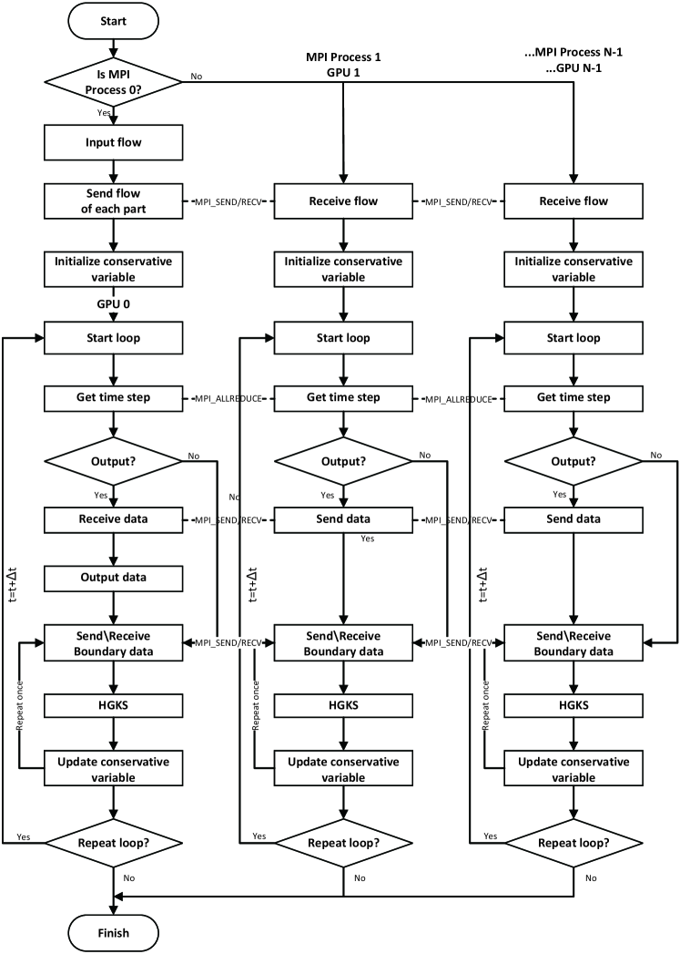
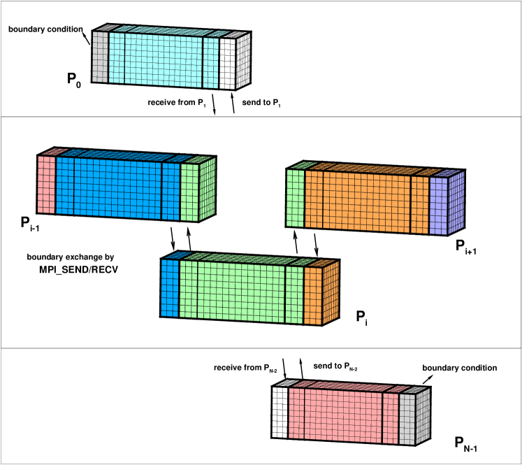
For the parallel computation with MPI, the domain decomposition are required for both CPU and GPU, where both one-dimensional (slab) and two-dimensional (pencil) decomposition are allowed. For CPU computation with MPI, hundreds or thousands of CPU cores are usually used in the computation, and the pencil decomposition can be used to improve the efficiency of data communications [23]. In terms of GPU computation with MPI, the slab decomposition is used, which reduces the frequency of GPU-GPU communications and improves performances. The domain decomposition and GPU-GPU communications are presented in Fig.3, where the computational domain is divided into parts in -direction and GPUs are used. For simplicity, denotes the -th MPI process, which deals with the tasks of -th decomposed computational domain in the -th GPU. To implement the WENO reconstruction, the processor exchanges the data with and using MPIRECV and MPISEND. The wall boundary condition of and can be implemented directly. For the periodic boundary, the data is exchanged between and using MPIRECV and MPISEND as well. In summary, the detailed data communication for GPU computation with MPI are shown in Algorithm.2. Fig.4 shows the HGKS code frame with multiple-GPUs. The initial data will be divided into parts according to domain decomposition and sent to corresponding process to using MPISEND. As for input and output, the MPI process is responsible for distributing data to other processors and collecting data from other processors, using MPISEND and MPIRECV. For each decomposed domain, the computation is executed with the prescribed GPU. The identical code is running for each GPU, where kernels and grids are similarly set as single-GPU code [29].
3.3 Detailed parameters of CPUs and GPUs
In following studies, the CPU codes run on the desktop with Intel Core i7-9700 CPU using OpenMP directives and TianHe-II supercomputer system with MPI and Intel mpiifort compiler, The HGKS codes with CPU are all compiled with FP64 precision. For the GPU computations, the Nvidia TITAN RTX GPU and Nvidia Tesla V100 GPU are used with Nvidia CUDA and Nvidia HPC SDK. The detailed parameters of CPU and GPU are given in Table.2 and Table.2, respectively. For TITAN RTX GPU, the GPU-GPU communication is achieved by connection traversing PCIe, and there are TITAN TRTX GPUs in one node. For Tesla V100 GPU, there are GPUs inside one GPU node, and more nodes are needed for more than GPUs. The GPU-GPU communication in one GPU node is achieved by Nvidia NVLink. The communication across GPU nodes can be achieved by Remote Direct Memory Access (RDMA) technique, including iWARP, RDMA over Converged Ethernet (RoCE) and InfiniBand. In this paper, RoCE is used for communication across GPU nodes.
As shown in Table.2, Tesla V100 is equipped with more FP64 precision cores and much stronger FP64 precision performance than TITAN RTX. For FP32 precision performance, two GPUs are comparable. Nvidia TITAN RTX is powered by Turing architecture, while Nvidia Tesla V100 is built to HPC by advanced Ampere architecture. Additionally, Tesla V100 outweighs TITAN RTX in GPU memory size and memory bandwidth. Thence, much excellent performance is excepted in FP64 precision simulation with Tesla V100. To validate the performance with FP32 and FP64 precision, numerical examples will be presented.
| CPU | Clock rate | Memory size | |
|---|---|---|---|
| Desktop | Intel Core i7-9700 | GHz | GB/ cores |
| TianHe-II | Intel Xeon E5-2692 v2 | GHz | GB/ cores |
| Nvidia TITAN RTX | Nvidia Tesla V100 | |
| Clock rate | 1.77 GHz | 1.53 GHz |
| Stream multiprocessor | 72 | 80 |
| FP64 core per SM | 2 | 32 |
| FP32 precision performance | 16.3 Tflops | 15.7 Tflops |
| FP64 precision performance | 509.8 Gflops | 7834 Gflops |
| GPU memory size | 24 GB | 32 GB |
| Memory bandwidth | 672 GB/s | 897 GB/s |
4 Numerical tests and discussions
Benchmarks for compressible turbulent flows, including Taylor-Green vortex and turbulent channel flows, are presented to validate the performance of multiple-GPU accelerated HGKS. In this section, we mainly concentrate on the computation with single-GPU and multiple-GPUs. The GPU-CPU comparison in terms of computational efficiency will be presented firstly, and the scalability of parallel multiple-GPU code will also be studied. Subsequently, HGKS implemented with GPUs is compiled with both FP32 and FP64 precision to evaluate the effect of precision on DNS of compressible turbulence. The detailed comparison on numerical efficiency and accuracy of statistical turbulent quantities with FP32 precision and FP64 precision is also presented.
4.1 Taylor-Green vortex for GPU-CPU comparison
Taylor-Green vortex (TGV) is a classical problem in fluid dynamics developed to study vortex dynamics, turbulent decay and energy dissipation process [35, 36, 37]. In this case, the detailed efficiency comparisons of HGKS running on the CPU and GPU will be given. The flow is computed within a periodic square box defined as . With a uniform temperature, the initial velocity and pressure are given by
In the computation, , and the Mach number takes , where is the sound speed. The fluid is a perfect gas with , Prandtl number , and Reynolds number . The characteristic convective time .
| Mesh size | Time step | i7-9700 | TITAN RTX | Tesla V100 | ||
|---|---|---|---|---|---|---|
| 0.757 | 0.126 | 6.0 | 0.047 | 16.1 | ||
| 11.421 | 1.496 | 7.6 | 0.714 | 16.0 | ||
| 182.720 | 24.256 | 7.4 | 11.697 | 15.4 |
In this section, GPU codes are all compiled with FP64 precision. To test the performance of single-GPU code, this case is run with Nvidia TITAN RTX and Nvidia Tesla V100 GPUs using Nvidia CUDA. As comparison, the CPU code running on the Intel Core i7-9700 is also tested. The execution times with different meshes are shown in Table.3, where the total execution time for CPU and GPUs are given in terms of hours and characteristic convective time are simulated. Due to the limitation of single GPU memory size, the uniform meshes with , and cells are used. For the CPU computation, cores are utilized with OpenMP parallel computation, and the corresponding execution time is used as the base for following comparisons. The speedups are also given in Table.3, which is defined as
where and denote the total execution time of CPU cores and GPU, respectively. Compared with the CPU code, 7x speedup is achieved by single TITAN RTX GPU and 16x speedup is achieved by single Tesla V100 GPU. Even though the Tesla V100 is approximately times faster than the TITAN RTX in FP64 precision computation ability, Tesla V100 only performs times faster than TITAN RTX. It indicates the memory bandwidth is the bottleneck for current memory-intensive simulations, and the detailed technique for GPU programming still required to be investigated.
| Mesh size | Time step | No. CPUs | |
|---|---|---|---|
| 16 | 13.3 | ||
| 256 | 13.5 | ||
| 1024 | 66 |
| Mesh size | No. GPUs | |||
|---|---|---|---|---|
| 1 | 11.697 | |||
| 2 | 6.201 | 6.122 | 0.079 | |
| 4 | 3.223 | 2.997 | 0.226 | |
| 8 | 1.987 | 1.548 | 0.439 | |
| 8 | 22.252 | 21.383 | 0.869 | |
| 12 | 19.055 | 17.250 | 1.805 | |
| 16 | 13.466 | 11.483 | 1.983 |
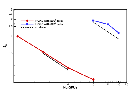
For single TITAN TRX with GB memory size, the maximum computation scale is cells. To enlarge the computational scale, the multiple-GPU accelerated HGKS are designed. Meanwhile, the parallel CPU code has been run on the TianHe-II supercomputer [23], and the execution times with respect to the number of CPU cores are presented in Table.4 for comparison. For the case with cells, the computational time of single Tesla V100 GPU is comparable with the MPI code with supercomputer using approximately Intel Xeon E5-2692 cores. For the case with cells, the computational time of CPU code with supercomputer using 1024 Intel Xeon E5-2692 cores is approximately times longer than that of GPU code using Tesla V100 GPUs. It can be inferred that the efficiency of GPU code with Tesla V100 GPUs approximately equals to that of MPI code with supercomputer cores, which agree well with the multiple-GPU accelerated finite difference code for multiphase flows [26]. These comparisons shows the excellent performance of multiple-GPU accelerated HGKS for large-scale turbulence simulation. To further show the performance of GPU computation, the scalability is defined as
| (9) |
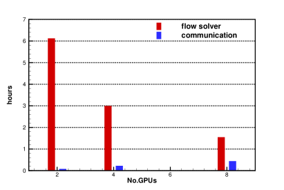
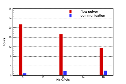
Fig.6 shows the log-log plot for and , where , and GPUs are used for the case with cells, while , and GPUs are used for the case with cells. The ideal scalability of parallel computations would be equal to . With the log-log plot for and , an ideal scalability would follow slope. However, such idea scalability is not possible due to the communication delay among the computational cores and the idle time of computational nodes associated with load balancing. As expected, the explicit formulation of HGKS scales properly with the increasing number of GPU. Conceptually, the total computation amount increases with a factor of , when the number of cells doubles in every direction. Taking the communication delay into account, the execution time of cells with 1 GPU approximately equals to that of cells with 16 GPUs, which also indicates the scalability of GPU code. When GPU code using more than GPUs, the communication across GPU nodes with RoCE is required, which accounts for the worse scalability using GPUs and GPUs. Table.5 shows the execution time in flow solver and the communication delay between CPU and GPU . Specifically, is consist of the time of WENO reconstruction, flux calculation at cell interface and update of flow variables, while concludes time for MPIRECV and MPISEND for initialization and boundary exchange, and MPIREDUCE for global time step. The histogram of and with different number of GPU is shown in Fig.6 with and cells. With the increase of GPU, more time for communication is consumed and the parallel efficiency is reduced accounting for the practical scalability in Fig.6. Especially, the communication across GPU nodes with RoCE is needed for the GPU code using more than GPUs, which consumes longer time than the communication in single GPU node with NVLink. The performance of communication across GPU nodes with InfiniBand will be tested, which is designed for HPC center to achieve larger throughout among GPU nodes.
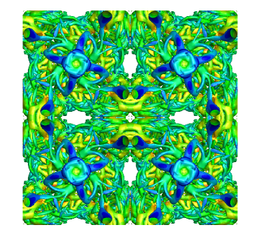
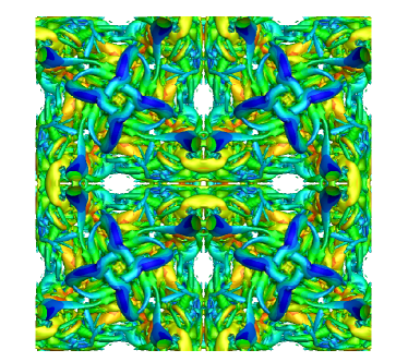
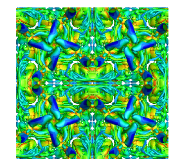
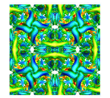
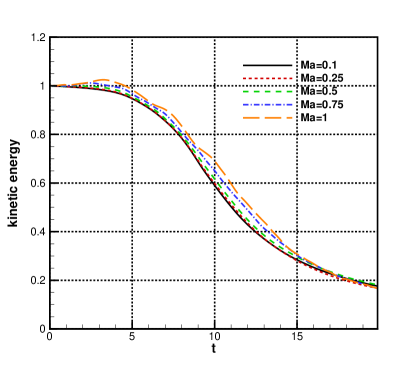
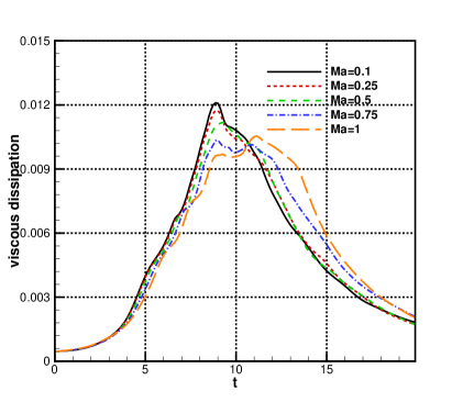
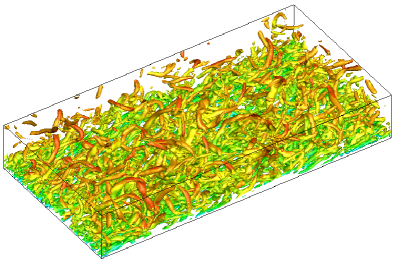
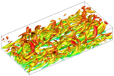
The time history of kinetic energy , dissipation rate and enstrophy dissipation rate of the above nearly incompressible case from GPU code is identical with the solution from previous CPU code, and more details can be found in [23]. With the efficient multiple-GPU accelerated platform, the compressible Taylor-Green vortexes with fixed Reynolds number Mach number , , and are also tested. Top view of Q-criterion with Mach number , , and at using cells are presented in Fig.7. The volume-averaged kinetic energy is given by
where is the volume of the computational domain. The total viscous dissipation is defined as
where is the coefficient of viscosity and . The time histories of kinetic energy and total viscous dissipation are given in Fig.8. Compared with the low Mach number cases, the transonic and supersonic cases with and have regions of increasing kinetic energy rather than a monotone decline. This is consistent with the compressible TGV simulations [38], where increases in the kinetic energy were reported during the time interval . A large spread of total viscous dissipation curves is observed in Fig.8, with the main trends being a delay and a flattening of the peak dissipation rate for increasing Mach numbers. The peak viscus dissipation rate for the curve matches closely to that of . Meanwhile, for the higher Mach number cases, the viscous dissipation rate is significantly higher in the late evolution region (i.e., ) than that from near incompressible case.
4.2 Turbulent channel flows for FP32-FP64 comparison
For most GPUs, the performance of FP32 precision is stronger than FP64 precision. In this case, to address the effect of FP32 and FP64 precision in terms of efficiency, memory costs and simulation accuracy, both the near incompressible and compressible turbulent channel flows are tested. Incompressible and compressible turbulent channel flows have been studied to understand the mechanism of wall-bounded turbulent flows [2, 4, 8]. In the computation, the physical domain is , and the computational mesh is given by the coordinate transformation
where the computational domain takes and . The fluid is initiated with density and the initial streamwise velocity profile is given by the perturbed Poiseuille flow profile, where the white noise is added with amplitude of local streamwise velocity. The spanwise and wall-normal velocity is initiated with white noise. The periodic boundary conditions are used in streamwise -direction and spanwise -directions, and the non-slip and isothermal boundary conditions are used in vertical -direction. The constant moment flux in the streamwise direction is used to determine the external force [23]. In current study, the nearly incompressible turbulent channel flow with friction Reynolds number and Mach number , and the compressible turbulent channel flow with bulk Reynolds number and bulk Mach number are simulated with the same set-up as previous studies [23, 39]. For compressible case, the viscosity is determined by the power law as , and the Prandtl number and are used. For the nearly incompressible turbulent channel flow, two cases and are tested, where and cells are distributed uniformly in the computational space as Table.7. For the compressible flow, two cases and are tested as well, where and cells are distributed uniformly in the computational space as Table.7. In the computation, the cases and are implemented with single GPU, while the cases and are implemented with double GPUs. Specifically, and are the minimum and maximum mesh space in the -direction. The equidistant meshes are used in and directions, and and are the equivalent plus unit, respectively. The fine meshes arrangement in case and can meet the mesh resolution for DNS in turbulent channel flows. The -criterion iso-surfaces for and are given Fig.9 in which both cases can well resolve the vortex structures. With the mesh refinement, the high-accuracy scheme corresponds to the resolution of abundant turbulent structures.
| Case | Mesh size | / | ||
|---|---|---|---|---|
| 0.93/12.80 | 9.69 | 9.69 | ||
| 0.45/6.40 | 9.69 | 9.69 |
| Case | Mesh size | / | ||
|---|---|---|---|---|
| 0.43/5.80 | 8.76 | 4.38 | ||
| 0.22/2.90 | 8.76 | 4.38 |
| TITAN RTX | with FP32 | with FP64 | |
| 0.414 | 1.152 | 2.783 | |
| 1.635 | 4.366 | 2.670 | |
| TITAN RTX | memory cost with FP32 | memory cost with FP64 | |
| 2.761 | 5.355 | 1.940 | |
| 5.087 | 10.009 | 1.968 | |
| Tesla V100 | with FP32 | with FP64 | |
| 0.377 | 0.642 | 1.703 | |
| 1.484 | 2.607 | 1.757 | |
| Tesla V100 | memory cost with FP32 | memory cost with FP64 | |
| 3.064 | 5.906 | 1.928 | |
| 5.390 | 10.559 | 1.959 |
Because of the reduction in device memory and improvement of arithmetic capabilities on GPUs, the benefits can be achieved by using FP32 precision compared to FP64 precision. In view of these strength, FP32-based and mixed-precision-based high-performance computing start to be explored [30, 31]. However, whether FP32 precision is sufficient for the DNS of turbulent flows still needs to be discussed. It is necessary to evaluate the effect of precision on DNS of compressible turbulence. Thus, the GPU-accelerated HGKS is compiled with FP32 precision and FP64 precision, and both nearly incompressible and compressible turbulent channel flows are used to test the performance in different precision. For simplicity, only the memory cost and computational time for the nearly incompressible cases are provided in Table.8, where the execution times are given in terms of hours and the memory cost is in GB. In the computation, two GPUs are used and statistical period is simulated. In Table.8, represents the speed up of with FP32 to with FP64, and denotes the ratio of memory cost with FP32 to memory cost with FP64. As expected, the memory of FP32 precision is about half of that of FP64 precision for both TITAN RTX and Tesla V100 GPUs. Compared with FP64-based simulation, 2.7x speedup is achieved for TITAN RTX GPU and 1.7x speedup is achieved for Tesla V100 GPU. As shown in Table.8, the comparable FP32 precision performance between TITAN RTX and Tesla V100 also provides comparable for these two GPUs. We conclude that Turing architecture and Ampere architecture perform comparably for memory-intensive computing tasks in FP32 precision.

To validate the accuracy of HGKS and address the effect with different precision, the statistical turbulent quantities are provided for the nearly incompressible and compressible turbulent channel flows. For FP32-FP64 comparison, all cases restarted from the same flow fields, and statistical periods are used to average the computational results for all cases. For the nearly incompressible channel flow, the logarithmic formulation is given by
| (10) |
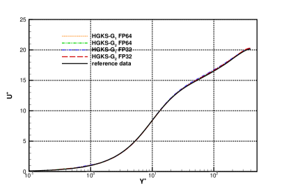
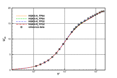
where the von Karman constant and is given for the low Reynolds number turbulent channel flow [2]. The mean streamwise velocity profiles with a log-linear plot are given in Fig.11, where the HGKS result is in reasonable agreement with the spectral results [4]. In order to account for the mean property of variations caused by compressibility, the Van Driest (VD) transformation [40] for the density-weighted velocity is considered
| (11) |
where represents the mean average over statistical periods and the X- and Z-directions. For the compressible flow, the transformed velocity is expected to satisfy the incompressible log law Eq.(10). The mean streamwise velocity profiles and with VD transformation as Eq.(11) are given in Fig.11 in log-linear plot. HGKS result is in reasonable agreement with the reference DNS solutions with the mesh refinements [9]. The mean velocity with FP32 and FP64 precision are also given in Fig.11 and Fig.11. It can be observed that the qualitative differences between different precision are negligible for statistical turbulent quantities with long time averaging.
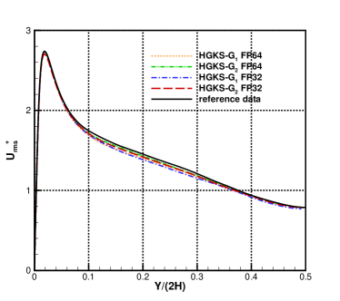
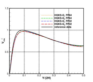
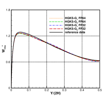
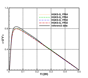
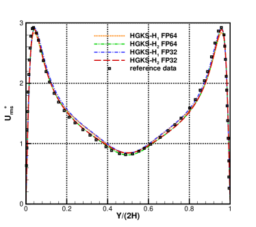
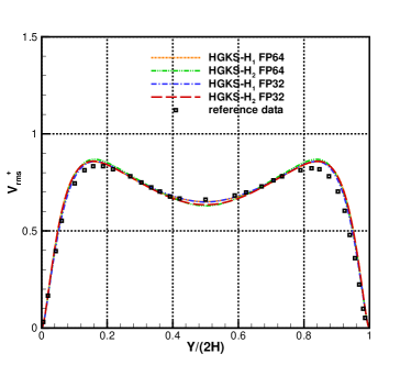
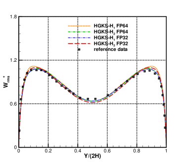
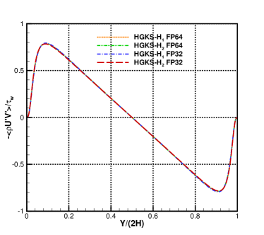
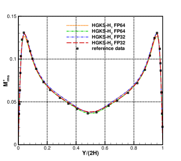
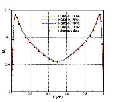
For the nearly incompressible turbulent channel flow, the time averaged normalized root-mean-square fluctuation velocity profile , , and normalized Reynolds stress profiles are given in Fig.12 for the cases and . The root mean square is defined as and , where represents the flow variables. With the refinement of mesh, the HGKS results are in reasonable agreement with the reference date, which given by the spectral method with cells [4]. It should also be noted that spectral method is for the exact incompressible flow, which provides accurate incompressible solution. The HGKS is more general for both nearly incompressible flows and compressible flows. For the compressible flow, the time averaged normalized root-mean-square fluctuation velocity profiles , , , Reynolds stress , the root-mean-square of Mach number and turbulent Mach number are presented in Fig.13 for the cases and . The turbulent Mach number is defined as , where and is the local sound speed. The results with agree well with the refereed DNS solutions, confirming the high-accuracy of HGKS for DNS in compressible wall-bounded turbulent flows. The statistical fluctuation quantities profiles with FP32 precision and FP64 precision are also given in Fig.12 and Fig.13. Despite the deviation of for different precision, the qualitative differences in accuracy between FP32 and FP64 precision are acceptable for statistical turbulent quantities with such a long time average.
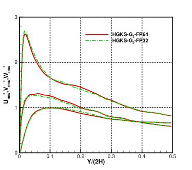
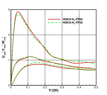
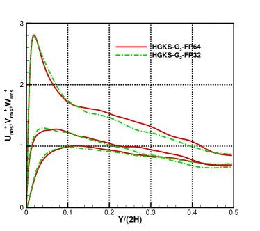
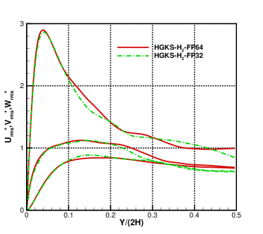
The instantaneous profiles of , , at and are shown in Fig.14 for the cases and with FP32 and FP64 precision, where cases restarted with the same initial flow field for each case. Compared with the time averaged profiles, the obvious deviations are observed for the instantaneous profiles. The deviations are caused by the round-off error of FP32 precision, which is approximately equals to or larger than the errors of numerical scheme. Since detailed effect of the round-off error is not easy to be analyzed, FP32 precision may not be safe for DNS in turbulence especially for time-evolutionary turbulent flows. In terms of the problems without very strict requirements in accuracy, such as large eddy simulation (LES) and Reynolds-averaged Navier–Stokes (RANS) simulation in turbulence, FP32 precision may be used due to its improvement of efficiency and reduction of memory. It also strongly suggests that the FP64 precision performance of GPU still requires to be improved to accommodate the increasing requirements of GPU-based HPC.
5 Conclusion
Based on the multi-scale physical transport and the coupled temporal-spatial gas evolution, the HGKS provides a workable tool for the numerical study of compressible turbulent flows. In this paper, to efficiently conduct large-scale DNS of turbulence, the HGKS code is developed with single GPU using CUDA architecture, and multiple GPUs using MPI and CUDA. The multiple GPUs are distributed across multiple CPUs at the cost of having to coordinate network communication via MPI. The Taylor-Green vortex problems and turbulent channel flows are presented to validate the performance of HGKS with multiple Nvidia TITAN RTX and Nvidia Tesla V100 GPUs. We mainly concentrate on the computational efficiency with single GPU and multiple GPUs, and the comparisons between FP32 precision and FP64 precision of GPU. For single-GPU computation, compared with the OpenMP CPU code using Intel Core i7-9700, 7x speedup is achieved by TITAN RTX and 16x speedup is achieved with Tesla V100. The computational time of single Tesla V100 GPU is comparable with the MPI code using supercomputer cores with Intel Xeon E5-2692. For multiple GPUs, the HGKS code scales properly with the number of GPU. It can be inferred that the efficiency of GPU code with Tesla V100 GPUs approximately equals to that of MPI code with CPU cores. Compared with FP64 precision simulation, the efficiency of HGKS can be improved and the memory is reduced with FP32 precision. However, with the long time computation in compressible turbulent channels flows, the differences in accuracy appear. Especially, the instantaneous statistical turbulent quantities is not acceptable using FP32 precision. The choice of precision should depend on the requirement of accuracy and the available computational resources. In the future, more challenging compressible flow problems, such as the supersonic turbulent boundary layer and the interaction of shock and turbulent boundary layer [41, 42], will be investigated with efficient multiple-GPU accelerated HGKS.
Ackonwledgement
This research is supported by National Natural Science Foundation of China (11701038), the Fundamental Research Funds for the Central Universities. We would thank Prof. Shucheng Pan of Northwestern Polytechnical University, Dr. Jun Peng and Dr. Shan Tang of Biren Technology for insightful discussions in GPU-based HPC.
References
- [1] S.B. Pope. Turbulent flows, Cambridge, (2001).
- [2] J. Kim, P. Moin, R. Moser, Turbulence statistics in fully developed channel flow at low Reynolds number, J. Fluid. Mech. 177 (1987) 133-166.
- [3] S. Chen, G. Doolen, J.R. Herring, R.H. Kraichnan, , et al. Far-dissipation range of turbulence. Physical review letters, 70(20) (1993), 3051.
- [4] R.D. Moser, J. Kim, N.N. Mansour, Direct numerical simulation of turbulent channel flow up to , Physics of Fluids 11 (1999) 943-945.
- [5] M. Lee, R. Moser, Direct numerical simulation of turbulent channel flow up to , J. Fluid. Mech. 774 (2015) 395-415.
- [6] J.C. Wang, L.P. Wang, Z.L. Xiao, Y. Shi, S.Y. Chen, A hybrid numerical simulation of isotropic compressible turbulence, J. Comput. Phys. 229 (2010) 5257-5279.
- [7] G.Y. Cao, L. Pan, K. Xu, Three dimensional high-order gas-kinetic scheme for supersonic isotropic turbulence I: Criterion for direct numerical simulation, Computers and Fluids 192 (2019) 104273.
- [8] G. Coleman, J. Kim, and R. Moser. A numerical study of turbulent supersonic isothermal-wall channel flow, J. Fluid. Mech. 305 (1995) 159-184.
- [9] D.X. Fu, Y.W. Ma, X.L. Li, Q. Wang, Direct numerical simulation of compressible turbulence, Science Press (2010).
- [10] Y. Ming, C.X. Xu, S. Pirozzoli, Genuine compressibility effects in wall-bounded turbulence. Physical Review Fluids 4.12 (2019) 123402.
- [11] S. Pirozzoli, F Grasso, T.B. Gatski, Direct numerical simulation and analysis of a spatially evolving supersonic turbulent boundary layer at , Physics of fluids 16 (2004) 530-545.
- [12] X. Liang, X.L. Li, D.X. Fu, Y.W. Ma, DNS and analysis of a spatially evolving hypersonic turbulent boundary layer over a flat plate at Mach 8, Sci. China Phys. Mech. Astron., 42 (2012) 282-293.
- [13] P.L. Bhatnagar, E.P. Gross, M. Krook, A Model for Collision Processes in Gases I: Small Amplitude Processes in Charged and Neutral One-Component Systems, Phys. Rev. 94 (1954) 511-525.
- [14] S. Chapman, T.G. Cowling, The Mathematical theory of Non-Uniform Gases, third edition, Cambridge University Press, (1990).
- [15] K. Xu, A gas-kinetic BGK scheme for the Navier-Stokes equations and its connection with artificial dissipation and Godunov method, J. Comput. Phys. 171 (2001) 289-335.
- [16] K. Xu, Direct modeling for computational fluid dynamics: construction and application of unified gas kinetic schemes, World Scientific (2015).
- [17] J.Q. Li, Z.F. Du, A two-stage fourth order time-accurate discretization for Lax-Wendroff type flow solvers I. hyperbolic conservation laws, SIAM J. Sci. Computing, 38 (2016) 3046-3069.
- [18] J.Q. Li, Two-stage fourth order: temporal-spatial coupling in computational fluid dynamics (CFD), Advances in Aerodynamics, (2019) 1:3.
- [19] L. Pan, K. Xu, Q.B. Li, J.Q. Li, An efficient and accurate two-stage fourth-order gas-kinetic scheme for the Navier-Stokes equations, J. Comput. Phys. 326 (2016) 197-221.
- [20] L. Pan, K. Xu, Two-stage fourth-order gas-kinetic scheme for three-dimensional Euler and Navier-Stokes solutions, Int. J. Comput. Fluid Dyn. 32 (2018) 395-411.
- [21] Y.Q. Yang, L. Pan, K. Xu, High-order gas-kinetic scheme on three-dimensional unstructured meshes for compressible flows, Physics of Fluids 33 (2021) 096102.
- [22] M.P.I. Forum, MPI: A Message-Passing Interface Standard, Version 2.2. High Performance Computing Center Stuttgart (2009).
- [23] G.Y. Cao, L. Pan, K. Xu, High-order gas-kinetic scheme with parallel computation for direct numerical simulation of turbulent flows, J. Comput. Phys. 448 (2022) 110739.
- [24] C.F. Xu, X.G. Deng, et el., Collaborating CPU and GPU for large-scale high-order CFD simulations with complex grids on the TianHe-1A supercomputer, J. Comput. Phys. 278 (2014) 275-297.
- [25] J. O’Connora, J.M. Dominguez, B.D. Rogers, S.J. Lind, P.K. Stansby, Eulerian incompressible smoothed particle hydrodynamics on multiple GPUs, Comput. Phys. Commun. 273 (2022) 108263.
- [26] Crialesi-Esposito, Marco, et al. FluTAS: A GPU-accelerated finite difference code for multiphase flows. arXiv preprint arXiv:2204.08834 (2022).
- [27] P. K. Yeung, K. Ravikumar, Advancing understanding of turbulence through extreme-scale computation: Intermittency and simulations at large problem sizes, Physical Review Fluids 5 (2020) 110517.
- [28] S. Pirozzoli, J. Romero, et el., One-point statistics for turbulent pipe flow up to , J. Fluid. Mech. 926 (2021).
- [29] Y.H. Wang, L. Pan, Three-dimensional discontinuous Galerkin based high-order gas-kinetic scheme and GPU implementation, Computers Fluids 55 (2022) 105510.
- [30] M. Lehmann, M.J. Krause, et al., On the accuracy and performance of the lattice Boltzmann method with 64-bit, 32-bit and novel 16-bit number formats, arXiv preprint arXiv:2112.08926 (2021).
- [31] A. Haidar, H. Bayraktar, et al., Mixed-precision iterative refinement using tensor cores on GPUs to accelerate solution of linear systems. Proceedings of the Royal Society A, 476(2243), 20200110.
- [32] G.S. Jiang, C.W. Shu, Efficient implementation of Weighted ENO schemes, J. Comput. Phys. 126 (1996) 202-228.
- [33] M. Castro, B. Costa, W. S. Don, High order weighted essentially non-oscillatory WENO-Z schemes for hyperbolic conservation laws, J. Comput. Phys. 230 (2011) 1766-1792.
- [34] J. Kraus, An Introduction to CUDA-Aware MPI. https://developer.nvidia.com/blog/introduction-cuda-aware-mpi/ (2013).
- [35] M.E. Brachet, D.I. Meiron, S.A. Orszag, B.G. Nickel, R.H. Morf, U. Frisch, Small-scale structure of the Taylor-Green vortex, J. Fluid. Mech. 130 (1983) 411-452.
- [36] J. Debonis, Solutions of the Taylor-Green vortex problem using high-resolution explicit finite difference methods, AIAA 2013-0382.
- [37] J. R. Bull, A. Jameson, Simulation of the compressible Taylor-Green vortex using high-order flux reconstruction schemes, AIAA 2014-3210.
- [38] N. Peng, Y. Yang, Effects of the Mach Number on the Evolution of Vortex-Surface Fields in Compressible Taylor-Green Flows, Physical Review Fluids, 3 (2018) 013401.
- [39] G.Y. Cao, L. Pan, K. Xu, S.Y. Chen, High-order gas-kinetic scheme in general curvilinear coordinate for iLES of compressible wall-bounded turbulent flows, arXiv.2107.08609.
- [40] P.G. Huang, and N. C. Gary, Van Driest transformation and compressible wall-bounded flows. AIAA journal 32 (1994) 2110-2113.
- [41] N. Adams, A. Direct simulation of the turbulent boundary layer along a compression ramp at and Reθ= 1685, J. Fluid. Mech. 420 (2000): 47-83.
- [42] M.W. Wu, M. Martin, Direct numerical simulation of supersonic turbulent boundary layer over a compression ramp, AIAA journal 45 (2007) 879-889.