This paper was converted on www.awesomepapers.org from LaTeX by an anonymous user.
Want to know more? Visit the Converter page.

Multilevel Richardson-Romberg and Importance Sampling in Derivative Pricing

Devang Sinha Department of Mathematics, Indian Institute of Technology Guwahati, Guwahati-781039, Assam, India, e-mail: [email protected]    Siddhartha P. Chakrabarty Department of Mathematics, Indian Institute of Technology Guwahati, Guwahati-781039, Assam, India, e-mail: [email protected], Phone: +91-361-2582606, Fax: +91-361-2582649
Abstract

In this paper, we propose and analyze a novel combination of multilevel Richardson-Romberg (ML2R) and importance sampling algorithm, with the aim of reducing the overall computational time, while achieving desired root-mean-squared error while pricing. We develop an idea to construct the Monte-Carlo estimator that deals with the parametric change of measure. We rely on the Robbins-Monro algorithm with projection, in order to approximate optimal change of measure parameter, for various levels of resolution in our multilevel algorithm. Furthermore, we propose incorporating discretization schemes with higher-order strong convergence, in order to simulate the underlying stochastic differential equations (SDEs) thereby achieving better accuracy. In order to do so, we study the Central Limit Theorem for the general multilevel algorithm. Further, we study the asymptotic behavior of our estimator, thereby proving the Strong Law of Large Numbers. Finally, we present numerical results to substantiate the efficacy of our developed algorithm.

Keywords: Multilevel Monte-Carlo Estimator; Richardson-Romberg Extrapolation; Importance Sampling; Path-dependent Functional; Option Pricing

1 Introduction

At the core of financial engineering lie the fundamental questions of pricing, portfolio management, and risk mitigation, which for all practical purposes, necessitates resorting to computational techniques, particularly, the Monte Carlo simulation approach. The emergence of this technique, as the key computational approach in the finance industry, can be attributed to the requirement of simulating high-dimensional stochastic models, which in turn is a result of the growth in computational complexity, pertaining to the dimension of the problem itself. More specifically, the main purpose of the usage of this procedure is to numerically approximate the expected value E(Y)E(Y), where Y=P(X)Y=P(X) is a functional of the random variable XX, with (in case of the concerned applications) XX being driven by a stochastic differential equation (SDE).

The increasing interest and application of the Monte Carlo approach in finance industry, can also be attributed to the development of Multilevel Monte Carlo (MLMC) technique, due to Giles [1], as it delivers remarkable improvement in computational complexity, over the standard Monte Carlo technique, in the biased framework. The interested readers may refer to the website of Giles ( http://people.maths.ox.ac.uk/~gilesm/mlmc_community.html) for an exhaustive and detailed listing of the flow of research concerning MLMC, both theoretical as well as application. The technique of MLMC draws its foundations from the technique of parametric integration, developed in [2], which was extended in [1], in order to construct a MLMC path method. While the control variate viewpoint used in [1] is similar to that of [2], however, unlike in case of [2], for the construction in [1], the random variable is infinite dimensional, with respect to the Brownian path, and there is no parametric integration that is involved. MLMC, as the name suggests, makes use of various levels of resolution, from the coarsest to the finest, where, from the perspective of the control variate, the simulation executed using the coarsest path, is used as a control variate, while carrying out the finer path based estimation. The introduction to MLMC was accomplished through the Euler-Maruyama discretization, a thorough analysis of which suggested that in order to estimate the variance of MLMC, one has to examine the strong convergence properties.

In another 2008 article [3], Giles presented a Milstein scheme for discretization of an SDE, an approach that led to improvement in the estimation of the variance. Further, it was demonstrated that, it could be more prudent to make use of different estimators for the coarser level and the finer level. The numerical results presented, as well as the thorough numerical analysis carried out in [4], demonstrates the efficacy of the method in case of option pricing problems. With the improvement in variance convergence, resulting from the usage of the Milstein scheme, the extension of the scheme in case of higher dimensional SDEs (involving the concept of Levy area) can be accomplished. However, in practice, there is no efficient way to simulate the Levy area, and the interested reader may refer to [5] for more discussion on this. In order to tackle this issue, the authors in [6], introduced the antithetic MLMC estimator, based on the classical antithetic variance reduction technique, wherein the idea of antithetic MLMC exploits the flexibility of the general MLMC estimator.

Giles and Waterhouse [7], published an extension of MLMC using Quasi-Monte Carlo (QMC) sample paths instead of Monte Carlo sample paths. The numerical results presented showed the effectiveness of QMC for SDE applications. However, the results presented in the paper were not supported by any theoretical development in this context. Nevertheless, recently, there has been some promising contribution towards the theoretical development of Quasi MLMC (QMLMC), for which one may refer to [8] and references therein. It has been shown that, under certain conditions, the QMLMC leads to multilevel methods, with a complexity which is O(ϵp)O(\epsilon^{-p}) with p<2p<2. In [9], Rhee and Glynn introduced a new approach of constructing an unbiased estimator, given a family of the biased estimators. The idea presented by them is closely related to that of MLMC, wherein the finest level of estimation is chosen, contingent on the level of accuracy. The results presented in [9] demonstrated a significant improvement in the computational cost over the standard MLMC. Also, they proved the square root convergence of the estimator, given that the strong order of convergence is greater than 12\displaystyle{\frac{1}{2}} for the path functionals.

2 Preliminaries

In this section we discuss the necessary preliminaries and assumptions, as a prelude to the comprehensive study of the algorithm developed in this work. We present a brief outline of Multilevel Richardson-Romberg estimator, introduced in [10] and recall the importance sampling algorithm in the context of the standard Monte-Carlo algorithm.

2.1 Multilevel Richardson-Romberg

In [1], Giles explored the Richardson extrapolation in the context of both the MLMC and the standard Monte Carlo. The MLMC on its own was significantly better than the Richardson extrapolation. However, taken together, they worked even better. Lemaire and Pages [10] took this approach and undertook further comprehensive error analysis. They combined the method developed in [1] and Multistep Richardson extrapolation in order to minimize the cost of simulation.

Suppose, we are interested in estimating the expected payoff value i.e., 𝔼(P(XT))\mathbb{E}\left(P(X_{T})\right) in an option pricing problem, with finite time horizon T>0T>0, where (Xt)0tT(X_{t})_{0\leq t\leq T} is a process with values in d\mathbb{R}^{d}, governed by the following SDE,

dXt=b(Xt)dt+j=1qσj(Xt)dWtj,X0=xd,dX_{t}=b(X_{t})dt+\sum\limits_{j=1}^{q}\sigma_{j}(X_{t})dW_{t}^{j},\leavevmode\nobreak\ X_{0}=x\in\mathbb{R}^{d}, (1)

where, W:=(W1W2Wq)W:=\begin{pmatrix}W_{1}&W_{2}&\dots&W_{q}\end{pmatrix} is a qq-dimensional Brownian motion on a filtered probability space
(Ω,(t)0tT,)\left(\Omega,(\mathcal{F}_{t}\right)_{0\leq t\leq T},\mathbb{P}), with b:ddb:\mathbb{R}^{d}\rightarrow\mathbb{R}^{d} and σj:dd\sigma_{j}:\mathbb{R}^{d}\rightarrow\mathbb{R}^{d} being the functions satisfying the following condition:

x,yd,|b(x)b(y)|+j=1q|σj(x)σj(y)|<Kb,σ|xy|,whereKb,σ>0.\forall x,y\in\mathbb{R}^{d},\leavevmode\nobreak\ \lvert b(x)-b(y)\rvert+\sum\limits_{j=1}^{q}\lvert\sigma_{j}(x)-\sigma_{j}(y)\rvert<K_{b,\sigma}\lvert x-y\rvert,\leavevmode\nobreak\ \text{where}\leavevmode\nobreak\ K_{b,\sigma}>0. (A.1)

The assumption (A.1) ensures the existence and uniqueness [11] of the strong solution of (1). Now, in order to estimate 𝔼(P(XT))\mathbb{E}\left(P(X_{T})\right) one should be able to simulate (Xt)0tT(X_{t})_{0\leq t\leq T}. However, except for a handful of cases, where one can devise an analytical or semi-analytical solution, we must resort to discretization schemes to perform the simulation. As discussed above, we use the Euler-Maruyama discretization scheme in order to simulate equation (1).

Let, MM\in\mathbb{N} be the refinement factor and let nl=Ml1n_{l}=M^{l-1}, where l=1,,Ll=1,\dots,L is the level refinement. Let hl=Tnl\displaystyle{h_{l}=\frac{T}{n_{l}}} be the time step size on level ll. For example, the Euler scheme on level ll is given by,

dXtnl=b(Xnlηnl(t))dt+j=1qσj(Xnlηnl(t))dWtj,l=1,,L,dX_{t}^{n_{l}}=b\left(X^{n_{l}}{\eta_{n_{l}(t)}}\right)dt+\sum\limits_{j=1}^{q}\sigma_{j}\left(X^{n_{l}}{\eta_{n_{l}(t)}}\right)dW_{t}^{j},\leavevmode\nobreak\ l=1,\dots,L,

where, ηnl(t):=t/hlhl\eta_{n_{l}(t)}:=\lfloor t/h_{l}\rfloor h_{l}. We approximate 𝔼[P(XT)]\mathbb{E}\left[P\left(X_{T}\right)\right] by 𝔼[P(XTnL)]\mathbb{E}\left[P\left(X_{T}^{n_{L}}\right)\right], where LL is the finest level. In [10] the authors proposed a methodology combining the order bias cancellation of Multilevel Richardson Romberg (ML2R), with variance control of MLMC, to solve the problem of improving the computational complexity, along with determining the optimal parameters in order to achieve the desired root-mean-squared error, with minimum computational effort. The study was based on weak error and strong error assumptions, on the sequence (P(XTh))h\left(P(X_{T}^{h})\right)_{h\in\mathcal{H}}, where ={𝐡n,n>1}\mathcal{H}=\left\{\frac{\mathbf{h}}{n},n>1\right\}. The assumptions [10, 11, 12] are stated as follows:

  1. (A)

    Weak Error:

    α>0,L¯1,(cl)1lL¯,𝔼[P(XTh)]𝔼[P(XT0)]=k=1L¯ckhαk+hαL¯ηL¯(h).\exists\alpha>0,\bar{L}\geq 1,(c_{l})_{1\leq l\leq\bar{L}},\quad\mathbb{E}[P(X^{h}_{T})]-\mathbb{E}[P(X^{0}_{T})]=\sum\limits_{k=1}^{\bar{L}}c_{k}h^{\alpha k}+h^{\alpha\bar{L}}\eta_{\bar{L}}(h). (2)
  2. (B)

    Strong Error:

    β>0,V11,P(XTh)P(XT0)22=𝔼[|P(XTh)P(XT0)|2]V1hβ.\exists\beta>0,V_{1}\geq 1,\|P(X^{h}_{T})-P(X^{0}_{T})\|^{2}_{2}=\mathbb{E}\left[|P(X^{h}_{T})-P(X^{0}_{T})|^{2}\right]\leq V_{1}h^{\beta}. (3)

With the consideration of the above assumptions, the ML2R estimator is defined as,

𝐉πN𝔼[P(XTnL)]=1N1k=1N1P(XTn1,k)+l=2LW~lNlk=1Nl(P(XTnl,k)P(XTnl1,k)),\mathbf{J}^{N}_{\pi}\coloneqq\mathbb{E}\left[P\left(X_{T}^{n_{L}}\right)\right]=\frac{1}{N_{1}}\sum\limits_{k=1}^{N_{1}}P\left(X_{T}^{n_{1},k}\right)+\sum\limits_{l=2}^{L}\frac{\widetilde{W}_{l}}{N_{l}}\sum\limits_{k=1}^{N_{l}}\left(P\left(X_{T}^{n_{l},k}\right)-P\left(X_{T}^{n_{l-1},k}\right)\right), (4)

where π=(h,μ,L)\pi=(h,\mu,L) are the optimal parameters obtained as the solution to,

(π(ϵ),N(ϵ))=argmin𝐉πN𝐉02ϵCost(𝐉πN).(\pi(\epsilon),N(\epsilon))={\arg\min}_{\|\mathbf{J}^{N}_{\pi}-\mathbf{J}_{0}\|_{2}\leq\epsilon}\text{Cost}(\mathbf{J}^{N}_{\pi}). (5)

where the cost function is given by [12],

Cost(𝐉πN)=Nhl=1Lμl(nl1+nl).\text{Cost}(\mathbf{J}^{N}_{\pi})=\frac{N}{h}\sum\limits_{l=1}^{L}\mu_{l}(n_{l-1}+n_{l}).

Further, in the above equation, NlN_{l} is the number of sample paths on level ll, and W~l\widetilde{W}_{l} are the weights given by,

W~l=j=lLwl,l=1,,L,\widetilde{W}_{l}=\sum\limits_{j=l}^{L}w_{l},\leavevmode\nobreak\ l=1,\dots,L, (6)

where w=(wl)1lL\textbf{w}=\left(w_{l}\right)_{1\leq l\leq L} is the solution to the Vandermonde system Vw=e1V\textbf{w}=e_{1}, with the Vandermonde matrix being defined by,

V=(1111n2αnLα1n2α(L1)nLα(L1))V=\begin{pmatrix}1&1&\dots&1\\ 1&n_{2}^{-\alpha}&\dots&n_{L}^{-\alpha}\\ \vdots&\vdots&\dots&\vdots\\ 1&n_{2}^{-\alpha(L-1)}&\dots&n_{L}^{-\alpha(L-1)}\\ \end{pmatrix} (7)

Here, α\alpha is the weak error rate as defined above. The interested reader may refer to [10] for the construction of the optimal parameters, as the closed solution to equation (5). Here we tabulate the explicit values of these parameters required to achieve the root-mean-squared error ϵ\epsilon, with the following constants being used:

  1. (A)

    λ=V1Var(P(XT0))andc~=limL|cL|1/α(0,)\displaystyle{\lambda=\sqrt{\frac{V_{1}}{\text{Var}\left(P(X^{0}_{T})\right)}}\leavevmode\nobreak\ \text{and}\leavevmode\nobreak\ \widetilde{c}_{\infty}=\lim_{L\rightarrow\infty}|c_{L}|^{1/\alpha}\in(0,\infty)}.

  2. (B)

    C¯M,β=1+Mβ/21+M1andC¯M,β=(1+Mβ/2)1+M1\displaystyle{\underline{C}_{M,\beta}=\frac{1+M^{\beta/2}}{\sqrt{1+M^{-1}}}\leavevmode\nobreak\ \text{and}\leavevmode\nobreak\ \overline{C}_{M,\beta}=\left(1+M^{\beta/2}\right)\sqrt{1+M^{-1}}}.

L(ϵ)L(\epsilon)
12+log(c~1/α𝐡)log(M)+(12+log(c~1/α𝐡)log(M))2+2log(A/ϵ)αlog(M)\left\lceil\frac{1}{2}+\frac{\log(\widetilde{c}_{\infty}^{1/\alpha}\mathbf{h})}{\log(M)}+\sqrt{\left(\frac{1}{2}+\frac{\log(\widetilde{c}_{\infty}^{1/\alpha}\mathbf{h})}{\log(M)}\right)^{2}+2\frac{\log(A/\epsilon)}{\alpha\log(M)}}\right\rceil
h(ϵ)h(\epsilon) 𝐡\mathbf{h}
μ(ϵ)\mu(\epsilon)
μ1=q(1+λhβ2)\mu_{1}=q^{*}(1+\lambda h^{\frac{\beta}{2}})
μl=qλhβ2C¯M,β|W~l(L,M)|M(1β)2(l1),l=2,,L\mu_{l}=q^{*}\lambda h^{\frac{\beta}{2}}\underline{C}_{M,\beta}|\widetilde{W}_{l}(L,M)|M^{-\frac{(1-\beta)}{2}(l-1)},l=2,\dots,L1lLμl=1\sum\limits_{1\leq l\leq L}\mu_{l}=1
N(ϵ)N(\epsilon)
(1+12αL)Var(P(XT0))(1+λhβ/2+λhβ/2C¯M,βl=2L|W~l(L,M)|M1β2(j1))ϵ2q\left(1+\frac{1}{2\alpha L}\right)\frac{\text{Var}\left(P(X^{0}_{T})\right)\left(1+\lambda h^{\beta/2}+\lambda h^{\beta/2}\overline{C}_{M,\beta}\sum\limits_{l=2}^{L}|\widetilde{W}_{l}(L,M)|M^{\frac{1-\beta}{2}(j-1)}\right)}{\epsilon^{2}q^{*}}
Table 1: Optimal parameters for the ML2R estimator

The above estimator was highly effective whenever there is a strong order of convergence i.e., β1\beta\leq 1, as it achieves O(ϵ2log(1/ϵ))O\left(\epsilon^{-2}\log(1/\epsilon)\right) for β=1\beta=1 and O(ϵ2e1βα2log(1/ϵ)log(M))O\left(\epsilon^{-2}e^{\frac{1-\beta}{\sqrt{\alpha}}\sqrt{2\log(1/\epsilon)\log(M)}}\right) for β<1\beta<1, contrary to O(ϵ2log(1/ϵ)2)O\left(\epsilon^{-2}\log(1/\epsilon)^{2}\right) and O(ϵ21βα)O\left(\epsilon^{-2-\frac{1-\beta}{\alpha}}\right), respectively, which is achieved by the standard MLMC.

2.2 Importance Sampling

Now following the idea of [13], we consider a parametric family of stochastic process (Xt(θ))0tT\left(X_{t}(\theta)\right)_{0\leq t\leq T}, with θd\theta\in\mathbb{R}^{d}, governed by the following SDE,

dXt(θ)=(b(Xt(θ))+σ(Xt(θ))θ)dt+j=1qσj(Xt(θ))dWtj,σ(x)=(σ1(x)σq(x)).dX_{t}(\theta)=(b(X_{t}(\theta))+\sigma(X_{t}(\theta))\theta)dt+\sum\limits_{j=1}^{q}\sigma_{j}(X_{t}(\theta))dW_{t}^{j},\leavevmode\nobreak\ \sigma(x)=\begin{pmatrix}\sigma_{1}(x)&\dots&\sigma_{q}(x)\end{pmatrix}. (8)

By the Girsanov’s Theorem, we know that there exists a probability measure θ\mathbb{P}_{\theta} equivalent to \mathbb{P} such that,

dθd|t=exp(θ,Wt12θ2t)𝒥(Wt,θ),\frac{d\mathbb{P}_{\theta}}{{d\mathbb{P}|}_{\mathcal{F}_{t}}}=\exp{\left(-\langle\theta,W_{t}\rangle-\frac{1}{2}\lVert\theta\rVert^{2}t\right)}\triangleq\mathcal{J}^{-}(W_{t},\theta), (9)

under which, the process (θt+Wt)0tT\left(\theta t+W_{t}\right)_{0\leq t\leq T} is a Brownian motion. Therefore,

𝔼[P(XT)]=𝔼θ[P(XT(θ))]=𝔼[P(XT(θ))𝒥(WT,θ)].\mathbb{E}_{\mathbb{P}}\left[P(X_{T})\right]=\mathbb{E}_{\mathbb{P}_{\theta}}\left[P(X_{T}(\theta))\right]=\mathbb{E}_{\mathbb{P}}\left[P(X_{T}(\theta))\mathcal{J}^{-}(W_{T},\theta)\right]. (10)

The efficiency of the Monte Carlo method is considerably dependent on how small the variance is in the process of estimation. Among the many variance reduction techniques, available in literature (for improvement of efficiency of the Monte Carlo method), importance sampling is one such variance reduction technique, which is known for its efficiency [14]. In general, the idea of parametric importance sampling is to introduce the parametric transformation such that θd\forall\theta\in\mathbb{R}^{d},

𝔼[P(XT)]=𝔼[h(θ,XT)].\mathbb{E}\left[P(X_{T})\right]=\mathbb{E}\left[h(\theta,X_{T})\right].

More specifically, we consider the general problem of estimating 𝔼[P(X)]\mathbb{E}[P(X)], where XX is a dd-dimensional random variable. Also if f(x)f(x) is the multivariate density, then,

𝔼[P(X)]=P(x)f(x)𝑑x=P(x+θ)f(x+θ)𝑑x=h(θ,x)f(x)𝑑x,\mathbb{E}[P(X)]=\int P(x)f(x)dx=\int P(x+\theta)f(x+\theta)dx=\int h(\theta,x)f(x)dx,

where h(θ,x)=P(x+θ)f(x+θ)f(x)\displaystyle{h(\theta,x)=\frac{P(x+\theta)f(x+\theta)}{f(x)}}. Now the idea of importance sampling Monte Carlo method is to estimate 𝔼(P(XT))\mathbb{E}\left(P(X_{T})\right), where θ\theta is given by,

θ=argminθdVar(P(XT(θ))𝒥(WT,θ)).\theta^{*}=\arg\min_{\theta\in\mathbb{R}^{d}}\text{Var}\leavevmode\nobreak\ \left(P(X_{T}(\theta))\mathcal{J}^{-}{(W_{T},\theta)}\right). (11)

In order to solve the above problem one can use the so-called Robbins-Monro algorithm that deals with a sequence of random variable (θi)i\left(\theta_{i}\right)_{i\in\mathbb{N}}, which approximates θ\theta^{*} accurately. However, the convergence of this algorithm requires restrictive conditions known as the non explosion condition given by [15],

𝔼[h2(θ,XT)]C(1+|θ|2)for allθd.\mathbb{E}[h^{2}\left(\theta,X_{T}\right)]\leq C\left(1+|\theta|^{2}\right)\leavevmode\nobreak\ \text{for all}\leavevmode\nobreak\ \theta\in\mathbb{R}^{d}.

To overcome these restrictive conditions, a truncation based procedure was introduced by Chen in [16, 17] which was furthered in [18, 19]. This was then proposed in the context of importance sampling [13]. An unconstrained procedure to approximate θ\theta^{*}, by using the regularity of the involved density extensively, was introduced in [20] along with the proof of the convergence of the algorithm.

The authors in [15] studied importance sampling in the context of statistical Romberg integration, which is a one-step generalization of the standard Monte Carlo integration. The paper used both constrained, as well as unconstrained optimization routines to approximate θ\theta^{*}. Further, they proved the almost sure convergence of both constrained and unconstrained versions of the optimization algorithm, towards the optimal parameter θ\theta^{*}, under discretized diffusion setting. The idea was then extended by [21] and [22] in the context of MLMC. The study carried out in [21] is the extension of [15] in the paradigm of MLMC. However [22] used sample average approximation to approximate θ\theta^{*}. Also, their algorithm performed an approximation procedure on each level of resolution, thus further enhancing the overall performance of the adaptive algorithm.

In this paper, we develop a hybrid algorithm incorporating ML2R and adaptive importance sampling procedure developed in [13] in the context of standard Monte Carlo in order to reduce the overall computational time, while achieving the desired accuracy. In [15], the authors studied the discretized version of the asymptotic variance obtained in the central limit theorem associated with the statistical Romberg method. The study was performed to determine the optimal parameter θ\theta^{*}, to minimize the variance of the Monte Carlo estimator. In [22], the authors extended the algorithm developed in [15] in the context of MLMC, building upon the Central Limit Theorem for the Euler MLMC studied in [23]. As discussed in [23], the optimal value of θ\theta is obtained by using a constrained and unconstrained version of the stochastic Robbins-Monro algorithm, whereas in [22] it is determined using deterministic Newton-Raphson’s method. However, the algorithm was developed in the context of Euler discretization, and only European option pricing was studied, with no reference to path-dependent functionals. In this paper, we develop upon the Central Limit Theorem, for the general multilevel approach studied in [12], that incorporates the results for path-dependent functionals as well. We look at the stochastic optimization approach to approximate θ\theta^{*}. Also, we use the Milstein scheme, as well as Euler in order to discretize the underlying SDE. In order to highlight the novelty and contribution of this work, we present a comparison of the work accomplished, with the existing literature, in Table 2

ML2R IS Hybrid Algorithm: (IS+MC Version) Euler Scheme Milstein Scheme Vanilla Option Exotic Option Reference Yes No No Yes No Yes Yes [10] No Yes Yes ( With Standard Monte carlo) Yes No Yes No [13] No Yes Yes (With MLMC) Yes No Yes No [22] No Yes Yes (With Statistical Romberg Integration) Yes No Yes No [15] No Yes Yes (Adaptive MLMC) Yes No Yes No [21] Yes Yes Yes Yes Yes Yes Yes Present Work

Table 2: Comparison between present work and previously existed studies based on various factors

3 Algorithm

In this paper, we follow the idea presented in [22] to develop our coupling algorithm, which we will refer to as AISML2R:

𝔼[P(XTnL)]\displaystyle\mathbb{E}\left[P\left(X_{T}^{n_{L}}\right)\right] =\displaystyle= 𝔼[P(XTn1(θ1))𝒥(WT1,θ1)]\displaystyle\mathbb{E}\left[P(X_{T}^{n_{1}}(\theta_{1}))\mathcal{J}^{-}(W^{1}_{T},\theta_{1})\right] (12)
+\displaystyle+ l=2LW~l𝔼[(P(XTnl(θl))P(XTnl1(θl))𝒥(WTl,θl)].\displaystyle\sum\limits_{l=2}^{L}\widetilde{W}_{l}\mathbb{E}\left[(P\left(X_{T}^{n_{l}}(\theta_{l})\right)-P\left(X_{T}^{n_{l-1}}(\theta_{l})\right)\mathcal{J}^{-}(W^{l}_{T},\theta_{l})\right].

By applying Monte Carlo method to each level ll with samples NlN_{l} in equation (12), we get,

𝐉πN,θ(θ1,,θL)\displaystyle\mathbf{J}_{\pi}^{N,\theta}\left(\theta_{1},\dots,\theta_{L}\right) =\displaystyle= 1N1k=1N1P(XT,θ1k1n1,k)𝒥(WT1,k,θ1k1)\displaystyle\frac{1}{N_{1}}\sum\limits_{k=1}^{N_{1}}P\left(X_{T,\theta_{1}^{k-1}}^{n_{1},k}\right)\mathcal{J}^{-}(W^{1,k}_{T},\theta_{1}^{k-1}) (13)
+\displaystyle+ l=2LW~lNlk=1Nl(P(XT,θlk1nl,k)P(XT,θlk1nl1,k))𝒥(WTl,k,θlk1).\displaystyle\sum\limits_{l=2}^{L}\frac{\widetilde{W}_{l}}{N_{l}}\sum\limits_{k=1}^{N_{l}}\left(P\left(X_{T,\theta_{l}^{k-1}}^{n_{l},k}\right)-P\left(X_{T,\theta_{l}^{k-1}}^{n_{l-1},k})\right)\mathcal{J}^{-}(W^{l,k}_{T},\theta_{l}^{k-1}\right).

In the above estimator, the value of θlk\theta^{k}_{l} on level ll, is calculated using the values of the payoff, and θlk1\theta^{k-1}_{l} obtained in the previous path simulation, using the stochastic approximation algorithm studied in Section 3.2 below, thus describing the adaptive nature of the algorithm.

3.1 Optimization Problem

In this subsection, we deal with the problem of finding the optimal value of θl\theta_{l}, to minimize the variance on level ll. For the sake of brevity, we let,

Y(h)(hM)β2(P(XTh/M)P(XTh))andYlY(𝐡Ml2).Y(h)\coloneqq\left(\frac{h}{M}\right)^{\frac{-\beta}{2}}\left(P\left(X^{h/M}_{T}\right)-P\left(X^{h}_{T}\right)\right)\leavevmode\nobreak\ \text{and}\leavevmode\nobreak\ Y_{l}\coloneqq Y\left(\frac{\mathbf{h}}{M^{l-2}}\right).

Further let,

Zl=P(XTh/Ml1)P(XTh/Ml2)andZ1=Y(𝐡)=P(XTn1).Z_{l}=P\left(X^{h/M^{l-1}}_{T}\right)-P\left(X^{h/M^{l-2}}_{T}\right)\leavevmode\nobreak\ \text{and}\leavevmode\nobreak\ Z_{1}=Y(\mathbf{h})=P(X_{T}^{n_{1}}).

We start our discussion by recalling the Central Limit Theorems for ML2R from [12],

Theorem 1 (Central Limit Theorem, β>1\beta>1).

Assume strong error for β>1\beta>1 and that (Y(h))h(Y(h))_{h\in\mathcal{H}} is L2L^{2}-uniformly integrable. We set:

σ12=1ΣVar(Y𝒉)Var(Y0)(1+λ𝒉β2)andσ22=1Σ𝒉β2l2M1β2(l1)Var(Yl)Var(Y0)V1C¯M,β,\sigma_{1}^{2}=\frac{1}{\Sigma}\frac{Var(Y_{\boldsymbol{h}})}{Var(Y_{0})\left(1+\lambda\boldsymbol{h}^{\frac{\beta}{2}}\right)}\leavevmode\nobreak\ \textit{and}\leavevmode\nobreak\ \sigma_{2}^{2}=\frac{1}{\Sigma}\frac{\boldsymbol{h}^{\frac{\beta}{2}}\sum\limits_{l\geq 2}M^{\frac{1-\beta}{2}(l-1)}Var(Y_{l})}{\sqrt{Var(Y_{0})V_{1}}\underline{C}_{M,\beta}},

with,

Σ=[1+λ𝒉β2(1+C¯M,βM1β21M1β2)],C¯M,β=1+Mβ21+M1,andC¯M,β=(1+Mβ2)1+M1.\Sigma=\left[1+\lambda\boldsymbol{h}^{\frac{\beta}{2}}\left(1+\overline{C}_{M,\beta}\frac{M^{\frac{1-\beta}{2}}}{1-M^{\frac{1-\beta}{2}}}\right)\right],\leavevmode\nobreak\ \underline{C}_{M,\beta}=\frac{1+M^{\frac{\beta}{2}}}{\sqrt{1+M^{-1}}},\leavevmode\nobreak\ \text{and}\leavevmode\nobreak\ \overline{C}_{M,\beta}=\left(1+M^{\frac{\beta}{2}}\right)\sqrt{1+M^{-1}}.

Assuming weak error for L¯1\bar{L}\geq 1, we have,

𝐉πN(ϵ)𝐉0ϵ𝒩(0,σ12+σ22),asϵ0.\frac{\mathbf{J}_{\pi}^{N}(\epsilon)-\mathbf{J}_{0}}{\epsilon}\xrightarrow{\mathcal{L}}\mathcal{N}(0,\sigma_{1}^{2}+\sigma_{2}^{2}),\leavevmode\nobreak\ \text{as}\epsilon\rightarrow 0.
Theorem 2 (Central Limit Theorem, 0<β10<\beta\leq 1).

Assume strong error for β(0,1]\beta\in(0,1] and that (Y(h))h(Y(h))_{h\in\mathcal{H}} is L2L^{2}-uniformly integrable. Assume furthermore limh0Y(h)22=v(M,β)\displaystyle{\lim_{h\rightarrow 0}\lVert Y(h)\rVert_{2}^{2}=v_{\infty}(M,\beta)}, we set:

σ2={v(M,β)(1+Mβ/2)2V11,if 2α>β,(v(M,β)c12(1Mβ/2)2)(1+Mβ/2)2V11,if 2α=β.\sigma^{2}=\begin{cases}v_{\infty}(M,\beta)\left(1+M^{\beta/2}\right)^{-2}V_{1}^{-1},\leavevmode\nobreak\ \text{if}\leavevmode\nobreak\ 2\alpha>\beta,\\ \left(v_{\infty}(M,\beta)-c_{1}^{2}(1-M^{\beta/2})^{2}\right)\left(1+M^{\beta/2}\right)^{-2}V_{1}^{-1},\leavevmode\nobreak\ \text{if}\leavevmode\nobreak\ 2\alpha=\beta.\end{cases}

Assuming weak error for L¯1\bar{L}\geq 1, we have,

𝐉πN(ϵ)𝐉0ϵ𝒩(0,σ2),asϵ0.\frac{\mathbf{J}_{\pi}^{N}(\epsilon)-\mathbf{J}_{0}}{\epsilon}\xrightarrow{\mathcal{L}}\mathcal{N}(0,\sigma^{2}),\leavevmode\nobreak\ \text{as}\leavevmode\nobreak\ \epsilon\rightarrow 0.

Based of the two theorems stated above we develop the optimization algorithm for β>1\beta>1 and β(0,1]\beta\in(0,1].

3.1.1 Case I:β>1\text{Case I:}\beta>1

In Theorem 1, let

σ12=k1Var(Y𝐡)andσl2=k2M1β2(l1)Var(Yl),\sigma_{1}^{2}=k_{1}\text{Var}(Y_{\mathbf{h}})\leavevmode\nobreak\ \text{and}\leavevmode\nobreak\ \sigma_{l}^{2}=k_{2}M^{\frac{1-\beta}{2}(l-1)}\text{Var}(Y_{l}),

where,

k1=1Σ1Var(Y0)(1+λ𝐡β2)andk2=𝐡β2ΣVar(Y0)V1C¯M,β,k_{1}=\frac{1}{\Sigma}\frac{1}{Var(Y_{0})(1+\lambda\mathbf{h}^{\frac{\beta}{2}})}\leavevmode\nobreak\ \text{and}\leavevmode\nobreak\ k_{2}=\frac{\mathbf{h}^{\frac{\beta}{2}}}{\Sigma\sqrt{Var(Y_{0})V_{1}}\underline{C}_{M,\beta}},

and therefore,

σ22=l2klVar(Yl)=l2σl2.\sigma_{2}^{2}=\sum\limits_{l\geq 2}k_{l}\text{Var}(Y_{l})=\sum\limits_{l\geq 2}\sigma_{l}^{2}.

From the practical point of view, it is necessary to use the truncated version of the above summation. In the thorough study carried out in [12], it was proven that for β>1\beta>1,

limL(ϵ)l=2L(ϵ)|W~lL(ϵ)|M1β2(l1)Var(Yl)=l=2M1β2(l1)Var(Yl).\lim_{L(\epsilon)\rightarrow\infty}\sum\limits_{l=2}^{L(\epsilon)}|\widetilde{W}_{l}^{L(\epsilon)}|M^{\frac{1-\beta}{2}(l-1)}\text{Var}(Y_{l})=\sum\limits_{l=2}^{\infty}M^{\frac{1-\beta}{2}(l-1)}\text{Var}(Y_{l}).

Therefore, owing to the above result and motivated by the analysis pertaining to the Central Limit Theorem carried out in [12], we can formulate the problem for l=1,,L(ϵ)l=1,\dots,L(\epsilon) as,

θl\displaystyle\theta_{l}^{*} =argminθlσl2\displaystyle={\arg\min}_{\theta_{l}\in\mathbb{R}}\sigma_{l}^{2} (14)
=argminθlk2M1β2(l1)|W~lL(ϵ)|Var[(Ylθ𝒥(WTl,θl))2]\displaystyle={\arg\min}_{\theta_{l}\in\mathbb{R}}k_{2}M^{\frac{1-\beta}{2}(l-1)}\lvert\widetilde{W}_{l}^{L(\epsilon)}\rvert\text{Var}\left[\left(Y^{\theta}_{l}\mathcal{J}^{-}(W^{l}_{T},\theta_{l})\right)^{2}\right]
=argminθlkl𝔼[((P(XT,θh/Ml1)P(XT,θh/Ml2))𝒥(WTl,θl))2],\displaystyle={\arg\min}_{\theta_{l}\in\mathbb{R}}k_{l}\mathbb{E}\left[\left(\left(P\left(X^{h/M^{l-1}}_{T,\theta}\right)-P\left(X^{h/M^{l-2}}_{T,\theta}\right)\right)\mathcal{J}^{-}(W^{l}_{T},\theta_{l})\right)^{2}\right],

where,

kl=k2M1+β2(l1)|W~lL(ϵ)|𝐡β.k_{l}=k_{2}M^{\frac{1+\beta}{2}(l-1)}\lvert\widetilde{W}_{l}^{L(\epsilon)}\rvert\mathbf{h}^{-\beta}. (15)

Using the Girsanov’s theorem, we can see that,

𝔼[((P(XT,θh/Ml1)P(XT,θh/Ml2))𝒥(WTl,θl))2]=𝔼[(P(XTh/Ml1)P(XTh/Ml2))2𝒥+(WTl,θl)],\mathbb{E}\left[\left(\left(P\left(X^{h/M^{l-1}}_{T,\theta}\right)-P\left(X^{h/M^{l-2}}_{T,\theta}\right)\right)\mathcal{J}^{-}(W^{l}_{T},\theta_{l})\right)^{2}\right]=\mathbb{E}\left[\left(P\left(X^{h/M^{l-1}}_{T}\right)-P\left(X^{h/M^{l-2}}_{T}\right)\right)^{2}\mathcal{J}^{+}(W^{l}_{T},\theta_{l})\right], (16)

where,

𝒥+(WTl,θl)=eWTl,θl+12θl2T.\mathcal{J}^{+}(W^{l}_{T},\theta_{l})=e^{-\langle W_{T}^{l},\theta_{l}\rangle+\frac{1}{2}\lVert\theta_{l}\rVert^{2}T}.

Similarly for l=1l=1, we have,

θ1=argminθ1k1𝔼[(Y2(𝐡)𝒥+(WT1,θ1))].\theta_{1}^{*}={\arg\min}_{\theta_{1}\in\mathbb{R}}k_{1}\mathbb{E}\left[\left(Y^{2}(\mathbf{h})\mathcal{J}^{+}(W^{1}_{T},\theta_{1})\right)\right]. (17)

3.1.2 Case II: β(0,1]\beta\in(0,1]

Based on Theorem 2, we define vlv_{\infty}^{l} be the level ll approximation of vv_{\infty}, where,

vl=Y(hMl2)22.v_{\infty}^{l}=\bigg{\lVert}Y\left(\frac{h}{M^{l-2}}\right)\bigg{\rVert}_{2}^{2}.

Therefore, we have,

σl2={vl(M,β)(1+Mβ/2)2V11,if 2α>β(vl(M,β)c12(1Mβ/2)2)(1+Mβ/2)2V11,if 2α=β.\sigma_{l}^{2}=\begin{cases}v_{\infty}^{l}(M,\beta)\left(1+M^{\beta/2}\right)^{-2}V_{1}^{-1},\leavevmode\nobreak\ \text{if}\leavevmode\nobreak\ 2\alpha>\beta\\ \left(v_{\infty}^{l}(M,\beta)-c_{1}^{2}(1-M^{\beta/2})^{2}\right)\left(1+M^{\beta/2}\right)^{-2}V_{1}^{-1},\leavevmode\nobreak\ \text{if}\leavevmode\nobreak\ 2\alpha=\beta.\end{cases} (18)

We follow the similar line of development as for β>1\beta>1 to formulate the problem for β(0,1]\beta\in(0,1]. As one can observe from (18) that, in order to minimize σl2\sigma^{2}_{l} on level ll, we only need to minimize vlv_{\infty}^{l}. Therefore, we formulate the optimization problem as follows ,

θl=argminθq𝔼[Yl2𝒥+(WTl,θl)].\theta_{l}^{*}=\arg\min_{\theta\in\mathbb{R}^{q}}\mathbb{E}\left[Y_{l}^{2}\mathcal{J}^{+}(W_{T}^{l},\theta_{l})\right]. (19)

3.2 Stochastic Algorithm

In this section we outline the stochastic approximation algorithm to estimate θl\theta_{l}^{*}. Based on the discussion in the previous section, we perform the discretization, such as Euler or Milstein, of the underlying SDE to approximate YlY_{l}’s. Whereas for stochastic approximation we resort to the Robbins-Monro algorithm, to approximate the value of θl,l=1,,L\theta_{l}^{*},\leavevmode\nobreak\ l=1,\dots,L. The aim is to construct a sequence of (θln)n(\theta_{l}^{n})_{n\in\mathbb{N}}, such that, limnθln=θl\displaystyle{\lim_{n\rightarrow\infty}\theta_{l}^{n}=\theta_{l}^{*}}.

Let Θq\Theta\subset\mathbb{R}^{q} be a compact convex subset such that θint(Θ)\theta\in\text{int}(\Theta). Then the sequence is constructed recursively as follows,

θln+1=ProjΘ[θlnγn+1Gl(θln,Yl,WT,l)],\theta_{l}^{n+1}=\text{Proj}_{\Theta}\bigg{[}\theta_{l}^{n}-\gamma_{n+1}G_{l}(\theta_{l}^{n},Y_{l},W_{T,l})\bigg{]}, (20)

where ProjΘ(θ)=minθΘ|θθ0|\displaystyle{\text{Proj}_{\Theta}(\theta)=\min_{\theta\in\Theta}\lvert\theta-\theta_{0}\rvert}. Also (γn)n1(\gamma_{n})_{n\geq 1} is a decreasing sequence of positive real numbers satisfying,

n=1γn=andi=1γn2<.\sum\limits_{n=1}^{\infty}\gamma_{n}=\infty\leavevmode\nobreak\ \text{and}\leavevmode\nobreak\ \sum\limits_{i=1}^{\infty}\gamma_{n}^{2}<\infty. (21)

where for β>1\beta>1,

Gl(θl,Yl,WTl)={(θlTWTl)klZl2𝒥+(WTl,θl),forl=2,,L,(θ1TWT1)k1Z12(𝐡)𝒥+(WT1,θ1),forl=1,G_{l}(\theta_{l},Y_{l},W^{l}_{T})=\bigg{\{}\begin{array}[]{ l l }\left(\theta_{l}T-W^{l}_{T}\right)k_{l}Z_{l}^{2}\mathcal{J}^{+}(W_{T}^{l},\theta_{l}),&\text{for}\leavevmode\nobreak\ l=2,\dots,L,\\ \left(\theta_{1}T-W^{1}_{T}\right)k_{1}Z_{1}^{2}(\mathbf{h})\mathcal{J}^{+}(W_{T}^{1},\theta_{1}),&\text{for}\leavevmode\nobreak\ l=1,\end{array} (22)

and for β(0,1]\beta\in(0,1],

Gl(θl,Yl,WTl)={(θlTWTl)Yl2𝒥+(WTl,θl),forl=2,,L,(θ1TWT1)Y2(𝐡)𝒥+(WT1,θ1),forl=1.G_{l}(\theta_{l},Y_{l},W^{l}_{T})=\bigg{\{}\begin{array}[]{ l l }\left(\theta_{l}T-W^{l}_{T}\right)Y_{l}^{2}\mathcal{J}^{+}(W_{T}^{l},\theta_{l}),&\text{for}\leavevmode\nobreak\ l=2,\dots,L,\\ \left(\theta_{1}T-W^{1}_{T}\right)Y^{2}(\mathbf{h})\mathcal{J}^{+}(W_{T}^{1},\theta_{1}),&\text{for}\leavevmode\nobreak\ l=1.\end{array} (23)

It may be noted that in this paper, we use the constrained version of the Robbins-Monro algorithm in order to estimate the approximate value of θl\theta_{l}^{*} for various level of resolutions.

4 Analysis

In this section we study our algorithm in detail. We start our discussion by establishing the existence and uniqueness of the θl\theta_{l}^{*} for various level of resolution. Further we carry out the asymptotic analysis of our AISML2R estimator, thereby establishing the Strong Law of Large Numbers.

4.1 Existence and Uniqueness of θl\theta_{l}^{*}.

Before, establishing the existence and uniqueness of θl\theta_{l}^{*}, we recall results related to the weights (W~l)l=1,,L(\widetilde{W}_{l})_{l=1,\dots,L}, from [12] necessary for our study. Accordingly, let us define,

al11k(l1)(1Mkα),l=1,,L,a_{l}\coloneqq\frac{1}{\prod_{1\leq k\leq(l-1)}\left(1-M^{-k\alpha}\right)},\leavevmode\nobreak\ l=1,\dots,L,
bl(1)lMαl(l+1)21k(l1)(1Mkα),l=0,,L.b_{l}\coloneqq(-1)^{l}\frac{M^{\frac{-\alpha l(l+1)}{2}}}{\prod_{1\leq k\leq(l-1)}\left(1-M^{-k\alpha}\right)},\leavevmode\nobreak\ l=0,\dots,L.

The following result was proved in [12],

Lemma 1.

Let α>0\alpha>0. and the associated weights (W~l)l=1,,L(\widetilde{W}_{l})_{l=1,\dots,L}, be as given in (6).

  1. (a)

    liml+al=a<+\lim_{l\rightarrow+\infty}a_{l}=a_{\infty}<+\infty and l=0+|bl|=B~<+\displaystyle{\sum\limits_{l=0}^{+\infty}\lvert b_{l}\rvert=\widetilde{B}_{\infty}<+\infty}.

  2. (b)

    The weights W~l\widetilde{W}_{l} are uniformly bounded,

    L,l{1,,L},|W~l|aB~.\forall L\in\mathbb{N}^{*},\forall l\in\{1,\dots,L\},\leavevmode\nobreak\ \lvert\widetilde{W}_{l}\rvert\leq a_{\infty}\widetilde{B}_{\infty}.
  3. (c)

    For every γ>0\gamma>0,

    limL+l=2L|W~l|Mγ(l1)=1Mγ1.\lim_{L\rightarrow+\infty}\sum\limits_{l=2}^{L}\lvert\widetilde{W}_{l}\rvert M^{-\gamma(l-1)}=\frac{1}{M^{\gamma}-1}.
  4. (d)

    Let vjj1{v_{j}}_{j\geq 1} be a bounded sequence of positive real numbers. Let γ\gamma\in\mathbb{R} and assume that limj+vj=1\lim_{j\rightarrow+\infty}v_{j}=1 when γ>0\gamma>0. Then the following limits hold:

    l=2L|W~l|Mγ(l1)vl{l2Mγ(l1)vl<+,forγ<0R,forγ=0,asL+MγLal1|k=0l1bk|Mγl,forγ>0.\sum\limits_{l=2}^{L}\lvert\widetilde{W}_{l}\rvert M^{\gamma(l-1)}v_{l}\sim\begin{cases}\sum\limits_{l\geq 2}M^{\gamma(l-1)}v_{l}<+\infty,\leavevmode\nobreak\ \text{for}\leavevmode\nobreak\ \gamma<0\\ R,\leavevmode\nobreak\ \text{for}\leavevmode\nobreak\ \gamma=0,\leavevmode\nobreak\ \text{as}\leavevmode\nobreak\ L\rightarrow+\infty\\ M^{\gamma L}a_{\infty}\sum\limits_{l\geq 1}\lvert\sum\limits_{k=0}^{l-1}b_{k}\rvert M^{-\gamma l},\textit{for}\leavevmode\nobreak\ \gamma>0.\end{cases}

With above results at our disposal, we present a series of results establishing the existence and uniqueness of the optimal parameter θl\theta_{l}^{*} on various level of resolution. For the most part the proof follows line of argument similar to that presented in [22, 15, 13]. We start our discussion bu proving the following lemma, necessary for the existence and uniqueness results.

Lemma 2.

Let p2p\geq 2 and assume the p\mathcal{L}^{p}-strong error rate assumption, i.e.,

β>0,V1(p)>0,P(XTh)P(XT)pp=𝔼[|P(XTh)P(XT)|p]V1(p)hβp/2,h.\exists\beta>0,V_{1}^{(p)}>0,\bigg{\lVert}P(X_{T}^{h})-P(X_{T})\bigg{\rVert}_{p}^{p}=\mathbb{E}\left[\bigg{\lvert}P(X_{T}^{h})-P(X_{T})\bigg{\rvert}^{p}\right]\leq V_{1}^{(p)}h^{\beta p/2},h\in\mathcal{H}. (24)

Then, 𝔼[sup|θ|c|Gl(θ,Yl,WT)|]<\mathbb{E}\left[\sup_{\lvert\theta\rvert\leq c}\bigg{\lvert}G_{l}(\theta,Y_{l},W_{T})\bigg{\rvert}\right]<\infty for l=2,,Ll=2,\dots,L and some constant c>0c>0\in\mathbb{R}.

Proof.

We prove the above lemma for β>1\beta>1. The proof for β(0,1]\beta\in(0,1] follows a similar line of argument and is relatively easy to prove. Consider,

|Gl(θ,Zl,WT)|=|(θTWT)klZl2eθ,WT+12|θ|2T|.\bigg{\lvert}G_{l}(\theta,Z_{l},W_{T})\bigg{\rvert}=\bigg{\lvert}(\theta T-W_{T})k_{l}Z_{l}^{2}e^{-\langle\theta,W_{T}\rangle+\frac{1}{2}\lvert\theta\rvert^{2}T}\bigg{\rvert}.

Then, for c>0c>0,

sup|θ|c|Gl(θ,Zl,WT)|\displaystyle\sup_{\lvert\theta\rvert\leq c}\bigg{\lvert}G_{l}(\theta,Z_{l},W_{T})\bigg{\rvert} =sup|θ|c|(θTWT)klZl2eθ,WT+12|θ|2T|,\displaystyle=\sup_{\lvert\theta\rvert\leq c}\bigg{\lvert}(\theta T-W_{T})k_{l}Z_{l}^{2}e^{-\langle\theta,W_{T}\rangle+\frac{1}{2}\lvert\theta\rvert^{2}T}\bigg{\rvert},
(cT+|WT|)klZl2ec|WT|+12|c|2T.\displaystyle\leq(cT+\lvert W_{T}\rvert)k_{l}Z_{l}^{2}e^{c\lvert W_{T}\rvert+\frac{1}{2}\lvert c\rvert^{2}T}.

Taking expectation on both sides and applying Hölder’s inequality for all p2p\geq 2, we get,

𝔼[sup|θ|c|Gl(θ,Yl,WT)|]ec22Tec|WT|(cT+|WT|)pp1klZl2p.\mathbb{E}\left[\sup_{\lvert\theta\rvert\leq c}\bigg{\lvert}G_{l}(\theta,Y_{l},W_{T})\bigg{\rvert}\right]\leq e^{\frac{c^{2}}{2}T}\bigg{\lVert}e^{c\lvert W_{T}\rvert}(cT+\lvert W_{T}\rvert)\bigg{\rVert}_{\frac{p}{p-1}}\bigg{\lVert}k_{l}Z_{l}^{2}\bigg{\rVert}_{p}.

It is clear that ec|WT|(cT+|WT|)pp1\bigg{\lVert}e^{c\lvert W_{T}\rvert}(cT+\lvert W_{T}\rvert)\bigg{\rVert}_{\frac{p}{p-1}} is bounded. As for klZl2p\lVert k_{l}Z_{l}^{2}\rVert_{p} we fallback to the p\mathcal{L}^{p}-strong error assumption. Therefore, we have,

klZl2p=klZl2p2K(M,β,h,p)klMβ(l1),\lVert k_{l}Z_{l}^{2}\rVert_{p}=k_{l}\lVert Z_{l}\rVert_{2p}^{2}\leq K(M,\beta,h,p)k_{l}M^{-\beta(l-1)}, (25)

where,

K(M,β,h,p)=(V1(2p))1p(1+Mβ2)2hβ.K(M,\beta,h,p)=\left(V_{1}^{(2p)}\right)^{\frac{1}{p}}\left(1+M^{\frac{\beta}{2}}\right)^{2}h^{\beta}. (26)

The boundedness of klMβ(l1)k_{l}M^{-\beta(l-1)} can be derived from the definition of klk_{l} and from (b) and (c) of Lemma 1. Hence, from the above analysis, we can conclude that, 𝔼[sup|θ|c|Gl(θ,Yl,WT)|]\mathbb{E}\left[\sup_{\lvert\theta\rvert\leq c}\bigg{\lvert}G_{l}(\theta,Y_{l},W_{T})\bigg{\rvert}\right] is bounded for l=2,,Ll=2,\dots,L. ∎

We state now, the result pertaining to the existence and uniqueness of optimal parameters on various level of resolutions.

Proposition 1.

Suppose bb and σ\sigma satisfies assumption (A.1). Let PP be such that,

(XTDP)=0,whereDP={x|Pis differentiable atx}.\mathbb{P}(X_{T}\notin D_{P})=0,\leavevmode\nobreak\ \text{where}\leavevmode\nobreak\ D_{P}=\{x\in\mathbb{R}|P\leavevmode\nobreak\ \text{is differentiable at}\leavevmode\nobreak\ x\}.

Further, if ZlZ_{l} satisfies the following conditions,

  1. (1)

    (Zl0)>0\mathbb{P}(Z_{l}\neq 0)>0.

  2. (2)

    Zl2p<+for somep>1\lVert Z_{l}^{2}\rVert_{p}<+\infty\leavevmode\nobreak\ \text{for some}\leavevmode\nobreak\ p>1.

Then the function θ𝐯l(θ)\theta\rightarrow\mathbf{v}_{l}(\theta) is 𝒞2\mathcal{C}^{2} and strictly convex with θ𝐯l(θ)=𝔼[Gl(θ,Zl,WT)]\nabla_{\theta}\mathbf{v}_{l}(\theta)=\mathbb{E}[G_{l}(\theta,Z_{l},W_{T})] for all ll\in\mathbb{N}. Moreover, there exists an unique θq\theta^{*}\in\mathbb{R}^{q} such that minθq𝐯l(θ)=𝐯l(θ)\min_{\theta\in\mathbb{R}^{q}}\mathbf{v}_{l}(\theta)=\mathbf{v}_{l}(\theta^{*}).

Proof.

To prove the proposition, we refer to the proof in [15, 22], in our context. Here we discuss the proof for l2l\geq 2 and β>1\beta>1. For l=1l=1 and β(0,1]\beta\in(0,1] the proofs are relatively easy and can be reproduced in the similar way. To begin with, one can observe that θkl(Zl)2eθ,WT+12|θ|2T\displaystyle{\theta\rightarrow k_{l}(Z_{l})^{2}e^{-\langle\theta,W_{T}\rangle+\frac{1}{2}\lvert\theta\rvert^{2}T}} is a continuously infinitely differentiable function with respect to θ\theta, and θj(kl(Zl)2eθ,WT+12|θ|2T)=kl(Zl)2(θjTWTj)eθ,WT+12|θ|2T\displaystyle{\frac{\partial}{\partial\theta^{j}}(k_{l}(Z_{l})^{2}e^{-\langle\theta,W_{T}\rangle+\frac{1}{2}\lvert\theta\rvert^{2}T})=k_{l}(Z_{l})^{2}(\theta^{j}T-W^{j}_{T})e^{-\langle\theta,W_{T}\rangle+\frac{1}{2}\lvert\theta\rvert^{2}T}}. Therefore, the first derivative of the map θkl(Zl)2eθ,WT+12|θ|2T\displaystyle{\theta\rightarrow k_{l}(Z_{l})^{2}e^{-\langle\theta,W_{T}\rangle+\frac{1}{2}\lvert\theta\rvert^{2}T}} is equal to Gl(θ,Zl,WT)G_{l}(\theta,Z_{l},W_{T}). As we have already seen in Lemma 2 that the supl𝔼[sup|θ|c|Gl(θ,Zl,WT)|]\sup_{l}\mathbb{E}[\sup_{\lvert\theta\rvert\leq c}\lvert G_{l}(\theta,Z_{l},W_{T})\rvert] is bounded, therefore by Lebesgue’s theorem we can conclude that 𝐯l(θ)\mathbf{v}_{l}(\theta) is 𝒞1(q)\mathcal{C}^{1}(\mathbb{R}^{q}), with θ𝐯l(θ)=𝔼[Gl(θ,Zl,WT)]\nabla_{\theta}\mathbf{v}_{l}(\theta)=\mathbb{E}[G_{l}(\theta,Z_{l},W_{T})] for all ll\in\mathbb{N}. A similar line of argument also proves that 𝐯l(θ)\mathbf{v}_{l}(\theta) is 𝒞2(q)\mathcal{C}^{2}(\mathbb{R}^{q}). The Hessian of 𝐯l(θ)\mathbf{v}_{l}(\theta) is given as follows,

Hess(𝐯l(θ))=𝔼[((θTWT)(θTWT)+TIq)kl(Zl)2eθ,WT+12|θ|2T].Hess(\mathbf{v}_{l}(\theta))=\mathbb{E}\left[\left((\theta T-W_{T})(\theta T-W_{T})^{*}+TI_{q}\right)k_{l}(Z_{l})^{2}e^{-\langle\theta,W_{T}\rangle+\frac{1}{2}\lvert\theta\rvert^{2}T}\right].

Since, (Zl0)>0\mathbb{P}(Z_{l}\neq 0)>0, therefore, for all uq{0}u\in\mathbb{R}^{q}\setminus\{0\}, uTHess(𝐯l(θ))u>0u^{T}Hess(\mathbf{v}_{l}(\theta))u>0. Hence, we can conclude that 𝐯l(θ)\mathbf{v}_{l}(\theta) is strictly convex. As a consequence, there exists a minimum θq\theta^{*}\in\mathbb{R}^{q}, such that minθq𝐯l(θ)=𝐯l(θ)\displaystyle{\min_{\theta\in\mathbb{R}^{q}}\mathbf{v}_{l}(\theta)=\mathbf{v}_{l}(\theta^{*})}. Further,the unique minimum is attained for a finite value of θ\theta, it is enough to prove that lim|θ|+𝐯l(θ)=+\displaystyle{\lim_{\lvert\theta\rvert\to+\infty}\mathbf{v}_{l}(\theta)=+\infty}. This can be proved using Fatou’s lemma as,

+=𝔼[lim inf|θ|+kl(Zl)2eθ,WT+12|θ|2T]lim inf|θ|+𝔼[kl(Zl)2eθ,WT+12|θ|2T].+\infty=\mathbb{E}\left[\liminf_{\lvert\theta\rvert\rightarrow+\infty}k_{l}(Z_{l})^{2}e^{-\langle\theta,W_{T}\rangle+\frac{1}{2}\lvert\theta\rvert^{2}T}\right]\leq\liminf_{\lvert\theta\rvert\rightarrow+\infty}\mathbb{E}\left[k_{l}(Z_{l})^{2}e^{-\langle\theta,W_{T}\rangle+\frac{1}{2}\lvert\theta\rvert^{2}T}\right].

This completes the proof. ∎

As the above proposition guarantees the existence and uniqueness of the θl\theta_{l}^{*} for various level of resolutions, we now state the main result proving the convergence of the sequence θlka.s.θl\theta_{l}^{k}\xrightarrow{a.s.}\theta_{l}^{*}, as kk\rightarrow\infty, under the assumptions of the Lemma 2 and Proposition 1.

Theorem 3.

If θl=argminθlq𝐯l(θ)\theta_{l}^{*}=\arg\min_{\theta_{l}\in\mathbb{R}^{q}}\mathbf{v}_{l}(\theta) is such that, θ𝐯l(θl)=0\nabla_{\theta}\mathbf{v}_{l}(\theta_{l}^{*})=0 and θlΘ\theta_{l}^{*}\in\Theta, then θlka.s.θl\theta_{l}^{k}\xrightarrow{a.s.}\theta_{l}^{*}, as kk\rightarrow\infty.

Proof.

To prove the above result we follow the assertion made in Theorem A.1 [24] that suggest that in order to prove θlkθl\theta_{l}^{k}\rightarrow\theta_{l}^{*}, where the sequence (θlk)k1(\theta_{l}^{k})_{k\geq 1} is constructed through a constrained version of the Robbins Monro, we need to verify two conditions, namely,

  1. (1)

    θθl,θ𝐯l(θ),θθl>0\forall\leavevmode\nobreak\ \theta\neq\theta_{l}^{*},\leavevmode\nobreak\ \langle\nabla_{\theta}\mathbf{v}_{l}(\theta),\theta-\theta_{l}^{*}\rangle>0.

  2. (2)

    Non explosion condition: C>0\exists\leavevmode\nobreak\ C>0 such that θΘ,𝔼[|Gl(θ,Zl,WT)|2]<C(1+|θ2|)\forall\theta\in\Theta,\leavevmode\nobreak\ \mathbb{E}\left[\lvert G_{l}(\theta,Z_{l},W_{T})\rvert^{2}\right]<C(1+\lvert\theta^{2}\rvert).

As we know, θ𝐯l(θl)=0\displaystyle{\nabla_{\theta}\mathbf{v}_{l}(\theta_{l}^{*})=0} and in the previous proposition it was proven that vlv_{l} is convex, therefore as a consequence, we prove that,

θθl,θ𝐯l(θ),θθl>0.\forall\theta\neq\theta_{l}^{*},\leavevmode\nobreak\ \langle\nabla_{\theta}\mathbf{v}_{l}(\theta),\theta-\theta_{l}^{*}\rangle>0. (27)

For the non-explosion condition, we use the Cauchy-Schwarz inquality,

𝔼[|Gl(θ,Zl,WT)|2]e|θ|2T(𝔼[kl4Zl8])12(𝔼[|eθ,WT(θTWT)|4])12.\mathbb{E}\left[\lvert G_{l}(\theta,Z_{l},W_{T})\rvert^{2}\right]\leq e^{\lvert\theta\rvert^{2}T}\left(\mathbb{E}[k_{l}^{4}Z_{l}^{8}]\right)^{\frac{1}{2}}\left(\mathbb{E}[\lvert e^{-\langle\theta,W_{T}\rangle}(\theta T-W_{T})\rvert^{4}]\right)^{\frac{1}{2}}. (28)

Under the assumption and following the similar line of argument of Lemma 2, it is easy to prove that there exists a constant C>0C>0, such that,

𝔼[|Gl(θ,Zl,WT)|2]e|θ|2TC(𝔼[|eθ,WT(θTWT)|4])12.\mathbb{E}\left[\lvert G_{l}(\theta,Z_{l},W_{T})\rvert^{2}\right]\leq e^{\lvert\theta\rvert^{2}T}C\left(\mathbb{E}[\lvert e^{-\langle\theta,W_{T}\rangle}(\theta T-W_{T})\rvert^{4}]\right)^{\frac{1}{2}}. (29)

Further using the fact the θΘ\theta\in\Theta, we can deduce that,

supθΘ𝔼[|Gl(θ,Zl,WT)|2]<.\sup_{\theta\in\Theta}\mathbb{E}\left[\lvert G_{l}(\theta,Z_{l},W_{T})\rvert^{2}\right]<\infty. (30)

which in turns concludes the non explosion condition. This proves the almost sure convergence of θlk\theta_{l}^{k} to θl\theta_{l}^{*} as kk\rightarrow\infty. ∎

4.2 Main Result

Theorem 4.

Let (θlk)k0Θ(\theta_{l}^{k})_{k\geq 0}\subset\Theta be a family of sequence converging to θlΘ\theta_{l}^{*}\in\Theta as kk\rightarrow\infty. Moreover for p2p\geq 2 assume weak error for all L1L\geq 1 and P(XT)𝐋pP(X_{T})\in\mathbf{L}^{p}. Furthermore assume the 𝐋p\mathbf{L}^{p}-strong error rate assumption,i.e.,

β>0,V1(p)>0,P(XTh)P(XT)pp=𝔼[|P(XTh)P(XT)|p]V1(p)hβp/2,h.\exists\beta>0,V_{1}^{(p})>0,\bigg{\lVert}P(X_{T}^{h})-P(X_{T})\bigg{\rVert}_{p}^{p}=\mathbb{E}\left[\bigg{\lvert}P(X_{T}^{h})-P(X_{T})\bigg{\rvert}^{p}\right]\leq V_{1}^{(p)}h^{\beta p/2},h\in\mathcal{H}. (31)

If (ϵk)k1(\epsilon_{k})_{k\geq 1} is a sequence of positive real numbers such that k1ϵkp<+\displaystyle{\sum\limits_{k\geq 1}\epsilon^{p}_{k}<+\infty}, then the AISML2R estimator satisfies,

𝐉πN,θa.s.𝐉0.\mathbf{J}_{\pi}^{N,\theta}\xrightarrow{a.s.}\mathbf{J}_{0}. (32)

We will assume the following notation,

𝐉~θ,π11N1k=1N1P(XT,θ1k1n1,k)𝒥(WT1,k,θ11,k1)𝔼[P(XTn1)]and𝐉~θ,π2l=2LW~lNlk=1NlY~l,θlk1k,\widetilde{\mathbf{J}}_{\theta,\pi}^{1}\coloneqq\frac{1}{N_{1}}\sum\limits_{k=1}^{N_{1}}P(X_{T,\theta^{k-1}_{1}}^{n_{1},k})\mathcal{J}^{-}(W_{T}^{1,k},\theta^{1,k-1}_{1})-\mathbb{E}\left[P(X_{T}^{n_{1}})\right]\leavevmode\nobreak\ \text{and}\leavevmode\nobreak\ \widetilde{\mathbf{J}}_{\theta,\pi}^{2}\coloneqq\sum\limits_{l=2}^{L}\frac{\widetilde{W}_{l}}{N_{l}}\sum\limits_{k=1}^{N_{l}}\widetilde{Y}_{l,\theta^{k-1}_{l}}^{k},

where we set,

Y~l,θl=(P(XT,θlnl)P(XT,θlnl1))𝒥(Wl,θl)𝔼[P(XTnl)P(XTnl1)],\widetilde{Y}_{l,\theta_{l}}=\left(P(X^{n_{l}}_{T,\theta_{l}})-P(X^{n_{l-1}}_{T,\theta_{l}})\right)\mathcal{J}^{-}(W_{l},\theta_{l})-\mathbb{E}\left[P(X^{n_{l}}_{T})-P(X^{n_{l-1}}_{T})\right], (33)

and

Y~1,θ1=(P(XT,θ1n1))𝒥(W1,θ1)𝔼[P(XTn1)].\ \widetilde{Y}_{1,\theta_{1}}=\left(P(X^{n_{1}}_{T,\theta_{1}})\right)\mathcal{J}^{-}(W_{1},\theta_{1})-\mathbb{E}\left[P(X^{n_{1}}_{T})\right]. (34)

Therefore, we have,

𝐉πN,θ𝐉0=𝐉~θ,π1+𝐉~θ,π2+𝔼[P(XTL)]𝐉0.\mathbf{J}_{\pi}^{N,\theta}-\mathbf{J}_{0}=\widetilde{\mathbf{J}}_{\theta,\pi}^{1}+\widetilde{\mathbf{J}}_{\theta,\pi}^{2}+\mathbb{E}[P(X_{T}^{L})]-\mathbf{J}_{0}.

A thorough analysis carried out in Section 4.2 of [12] shows that the last term in the equation converges to zero as ϵ\epsilon\rightarrow\infty. We start our discussion by proving the following lemma.

Lemma 3.

Let p2p\geq 2 and |θ|c\lvert\theta\rvert\leq c. Then there exist a positive constant K1(M,β,p,c)K_{1}(M,\beta,p,c) such that,

Y~l,θppK1(M,β,p,c)Mβp(l1)/2,l=2,,L.\lVert\widetilde{Y}_{l,\theta}\rVert_{p}^{p}\leq K_{1}(M,\beta,p,c)M^{-\beta p(l-1)/2},\leavevmode\nobreak\ l=2,\dots,L.
Proof.

By Minkowski’s Inequality, we have,

(𝔼[|Y~l,θ)|p])1/p\displaystyle\left(\mathbb{E}\left[|\widetilde{Y}_{l,\theta})|^{p}\right]\right)^{1/{p}} (P(XT,θnl)P(XT,θnl1))𝒥(WTl,θ)p+|𝔼[P(XTnl)P(XTnl1)]|,\displaystyle\leq\biggl{\lVert}\left(P(X^{n_{l}}_{T,\theta})-P(X^{n_{l-1}}_{T,\theta})\right)\mathcal{J}^{-}(W^{l}_{T},\theta)\biggr{\rVert}_{p}+\biggl{\lvert}\mathbb{E}\left[P(X^{n_{l}}_{T})-P(X^{n_{l-1}}_{T})\right]\biggr{\rvert}, (35)
(P(XT,θnl)P(XT,θnl1))𝒥(WTl,θ)pI+[P(XTnl)P(XTnl1)]pII.\displaystyle\leq\underbrace{\biggl{\lVert}\left(P(X^{n_{l}}_{T,\theta})-P(X^{n_{l-1}}_{T,\theta})\right)\mathcal{J}^{-}(W^{l}_{T},\theta)\biggr{\rVert}_{p}}_{\text{I}}+\underbrace{\biggl{\lVert}\left[P(X^{n_{l}}_{T})-P(X^{n_{l-1}}_{T})\right]\biggr{\rVert}_{p}}_{\text{II}}.

In order to bound (I)(\textit{I}) of (35), we apply the Holder’s Inequality,

(P(XT,θnl)P(XT,θnl1))𝒥(WTl,θ)pp\displaystyle\biggl{\lVert}\left(P(X^{n_{l}}_{T,\theta})-P(X^{n_{l-1}}_{T,\theta})\right)\mathcal{J}^{-}(W^{l}_{T},\theta)\biggr{\rVert}_{p}^{p} =𝔼[|(P(XT,θnl)P(XT,θnl1))𝒥(WTl,θ)|p],\displaystyle=\mathbb{E}\left[\bigg{\lvert}\left(P(X_{T,\theta}^{n_{l}})-P(X_{T,\theta}^{n_{l-1}})\right)\mathcal{J}^{-}(W^{l}_{T},\theta)\bigg{\rvert}^{p}\right], (36)
=𝔼[|(P(XTnl)P(XTnl1))|p(𝒥+(WTl,θ))p1],\displaystyle=\mathbb{E}\left[\bigg{\lvert}\left(P(X_{T}^{n_{l}})-P(X_{T}^{n_{l-1}})\right)\bigg{\rvert}^{p}\left(\mathcal{J}^{+}(W^{l}_{T},\theta)\right)^{p-1}\right],
(𝔼[|(P(XTnl)P(XTnl1))|p2])1p(𝒥+(WTl,θ))p1pp1,\displaystyle\leq\left(\mathbb{E}\left[\bigg{\lvert}\left(P(X_{T}^{n_{l}})-P(X_{T}^{n_{l-1}})\right)\bigg{\rvert}^{p^{2}}\right]\right)^{\frac{1}{p}}\bigg{\lVert}\left(\mathcal{J}^{+}(W^{l}_{T},\theta)\right)^{p-1}\bigg{\rVert}_{\frac{p}{p-1}},
e(p21)2c2TP(XTnl)P(XTnl1)p2p.\displaystyle\leq e^{\frac{(p^{2}-1)}{2}c^{2}T}\bigg{\lVert}P(X_{T}^{n_{l}})-P(X_{T}^{n_{l-1}})\bigg{\rVert}_{p^{2}}^{p}.

Therefore, from above analysis, we have,

(P(XT,θnl)P(XT,θnl1))𝒥(WTl,θ)pe(p21)2pc2TP(XTnl)P(XTnl1)p2.\biggl{\lVert}\left(P(X^{n_{l}}_{T,\theta})-P(X^{n_{l-1}}_{T,\theta})\right)\mathcal{J}^{-}(W^{l}_{T},\theta)\biggr{\rVert}_{p}\leq e^{\frac{(p^{2}-1)}{2p}c^{2}T}\bigg{\lVert}P(X_{T}^{n_{l}})-P(X_{T}^{n_{l-1}})\bigg{\rVert}_{p^{2}}. (37)

Further for (II)(II) of (35), the assumption (31) yields,

[P(XTnl)P(XTnl1)]ppV1(p)(1+Mβ/2)p𝐡βp/2Mβp(l1)/2.\biggl{\lVert}\left[P(X^{n_{l}}_{T})-P(X^{n_{l-1}}_{T})\right]\biggr{\rVert}_{p}^{p}\leq V_{1}^{(p)}(1+M^{\beta/2})^{p}\mathbf{h}^{\beta p/2}M^{-\beta p(l-1)/2}. (38)

Now from (35) and (37), we get,

(𝔼[|Y~l,θ)|p])1/p(1+e(p21)2pc2T)P(XTnl)P(XTnl1)p2.\left(\mathbb{E}\left[\lvert\widetilde{Y}_{l,\theta})\rvert^{p}\right]\right)^{1/{p}}\leq\left(1+e^{\frac{(p^{2}-1)}{2p}c^{2}T}\right)\bigg{\lVert}P(X_{T}^{n_{l}})-P(X_{T}^{n_{l-1}})\bigg{\rVert}_{p^{2}}. (39)

Combining above inequality and (38) yields,

Y~l,θppK1(M,β,p,c)Mβp(l1)/2,\lVert\widetilde{Y}_{l,\theta}\rVert_{p}^{p}\leq K_{1}(M,\beta,p,c)M^{-\beta p(l-1)/2}, (40)

where,

K1(M,β,p,c)=(1+e(p21)2pc2T)(V1(p2))1/p(1+Mβ/2)p𝐡βp/2.K_{1}(M,\beta,p,c)=\left(1+e^{\frac{(p^{2}-1)}{2p}c^{2}T}\right)\left(V_{1}^{(p^{2})}\right)^{1/p}(1+M^{\beta/2})^{p}\mathbf{h}^{\beta p/2}.

Proposition 2.

Let p2p\geq 2 and θlkΘ\theta_{l}^{k}\in\Theta for l=2,,Ll=2,\dots,L and kk\in\mathbb{N}^{*}. Then there exists a constant K2(M,β,p,c)K_{2}(M,\beta,p,c), such that,

𝔼[|𝐉~θ,π2,ϵ|p]K2(M,β,p,c)ϵpfor some constantc>0.\mathbb{E}\left[\lvert\widetilde{\mathbf{J}}_{\theta,\pi}^{2,\epsilon}\rvert^{p}\right]\leq K_{2}(M,\beta,p,c)\epsilon^{p}\leavevmode\nobreak\ \text{for some constant}\leavevmode\nobreak\ c>0. (41)
Proof.

We start our discussion by observing that as θlkΘ\theta_{l}^{k}\in\Theta, there exists a positive constant cc such that |θlk|c,k\lvert\theta_{l}^{k}\rvert\leq c,\leavevmode\nobreak\ \forall k\in\mathbb{N}. Now, we define the following filtration (T,k)k1\left(\mathcal{F}_{T,k}\right)_{k\geq 1}, where T,kσ(Wt,j,jk,tT)\mathcal{F}_{T,k}\coloneqq\sigma(W_{t,j},\leavevmode\nobreak\ j\leq k,t\leq T). With this filtration, one can readily observe that k=1jY~l,θlk1k\displaystyle{\sum\limits_{k=1}^{j}\widetilde{Y}_{l,\theta_{l}^{k-1}}^{k}} is a martingale with respect to T,j\mathcal{F}_{T,j}. Now consider the following definition,

slk=1NlY~l,θlk1k,forl=2,,L.s_{l}\coloneqq\sum\limits_{k=1}^{N_{l}}\widetilde{Y}_{l,\theta_{l}^{k-1}}^{k},\leavevmode\nobreak\ \text{for}\leavevmode\nobreak\ l=2,\dots,L. (42)

Since k=1jY~l,θlk1k\displaystyle{\sum\limits_{k=1}^{j}\widetilde{Y}_{l,\theta_{l}^{k-1}}^{k}} is T,j\mathcal{F}_{T,j} martingale, therefore by Rosenthal’s inequality [25], we have,

slppCp{𝔼[k=1Nl𝔼[(Y~l,θlk1)2|T,k1]]p/2+k=1Nl𝔼[|Y~l,θlk1|p]}.\lVert s_{l}\rVert_{p}^{p}\leq C_{p}\left\{\mathbb{E}\left[\sum\limits_{k=1}^{N_{l}}\mathbb{E}[(\widetilde{Y}_{l,\theta_{l}^{k-1}})^{2}|\mathcal{F}_{T,k-1}]\right]^{p/2}+\sum\limits_{k=1}^{N_{l}}\mathbb{E}\left[\lvert\widetilde{Y}_{l,\theta_{l}^{k-1}}\rvert^{p}\right]\right\}. (43)

Now, from the previous Lemma, one can easily conclude that,

k=1Nl𝔼[|Y~l,θlk1|p]NlK1Mβp(l1)/2.\sum\limits_{k=1}^{N_{l}}\mathbb{E}\left[\lvert\widetilde{Y}_{l,\theta_{l}^{k-1}}\rvert^{p}\right]\leq N_{l}K_{1}M^{-\beta p(l-1)/2}. (44)

As for the first term, we use Theorem A.8 of [25], to obtain,

𝔼[k=1Nl𝔼[(Y~l,θlk1)2|T,k1]]p/2\displaystyle\mathbb{E}\left[\sum\limits_{k=1}^{N_{l}}\mathbb{E}\left[(\widetilde{Y}_{l,\theta_{l}^{k-1}})^{2}|\mathcal{F}_{T,k-1}\right]\right]^{p/2} Ap𝔼[k=1Nl(Y~l,θlk1)2]p/2=Apk=1Nl(Y~l,θlk1)2p/2p/2\displaystyle\leq A_{p}\mathbb{E}\left[\sum\limits_{k=1}^{N_{l}}(\widetilde{Y}_{l,\theta_{l}^{k-1}})^{2}\right]^{p/2}=A_{p}\bigg{\lVert}\sum\limits_{k=1}^{N_{l}}(\widetilde{Y}_{l,\theta_{l}^{k-1}})^{2}\bigg{\rVert}_{p/2}^{p/2} (45)
Ap(k=1Nl(Y~l,θlk1)2p/2)p/2Ap(Nl)p/2K1Mβp(l1)/2,\displaystyle\leq A_{p}\left(\sum\limits_{k=1}^{N_{l}}\lVert(\widetilde{Y}_{l,\theta_{l}^{k-1}})^{2}\rVert_{p/2}\right)^{p/2}\leq A_{p}(N_{l})^{p/2}K_{1}M^{-\beta p(l-1)/2},

where the last inequality is the consequence of the previous Lemma. Therefore, we have for p2p\geq 2,

slpp\displaystyle\lVert s_{l}\rVert^{p}_{p} Cp{Ap(Nl)p/2K1Mβp(l1)/2+NlK1Mβp(l1)/2}\displaystyle\leq C_{p}\left\{A_{p}(N_{l})^{p/2}K_{1}M^{-\beta p(l-1)/2}+N_{l}K_{1}M^{-\beta p(l-1)/2}\right\} Cp{2Ap(Nl)p/2K1Mβp(l1)/2}.\displaystyle\leq C_{p}\left\{2A_{p}(N_{l})^{p/2}K_{1}M^{-\beta p(l-1)/2}\right\}. (46)

Now, let KpCpApK1K_{p}\coloneqq C_{p}A_{p}K_{1}. Therefore, we have,

𝔼[|sl|p](Kp(Nl)p/2Mβp(l1)/2).\mathbb{E}[\lvert s_{l}\rvert^{p}]\leq\left(K_{p}(N_{l})^{p/2}M^{-\beta p(l-1)/2}\right). (47)

Now, consider the following,

𝔼[|𝐉~θ,π2|p]=𝔼[|l=2LW~lNl𝐬l|p].\mathbb{E}\left[\lvert\widetilde{\mathbf{J}}_{\theta,\pi}^{2}\rvert^{p}\right]=\mathbb{E}\left[\bigg{\lvert}\sum\limits_{l=2}^{L}\frac{\widetilde{W}_{l}}{N_{l}}\mathbf{s}_{l}\bigg{\rvert}^{p}\right]. (48)

As one can observe that, (sl)l2(s_{l})_{l\geq 2} are independent random variable in ll, therefore, by a version of Rosenthal’s inequality [25], we have,

𝔼[|l=2LW~lNlsl|p]\displaystyle\mathbb{E}\left[\bigg{\lvert}\sum\limits_{l=2}^{L}\frac{\widetilde{W}_{l}}{N_{l}}s_{l}\bigg{\rvert}^{p}\right] δp{(l=2L𝔼[W~lNlsl]2)p/2+l=2L𝔼[|W~lNlsl|p]}\displaystyle\leq\delta_{p}\left\{\left(\sum\limits_{l=2}^{L}\mathbb{E}\left[\frac{\widetilde{W}_{l}}{N_{l}}s_{l}\right]^{2}\right)^{p/2}+\sum\limits_{l=2}^{L}\mathbb{E}\left[\bigg{\lvert}\frac{\widetilde{W}_{l}}{N_{l}}s_{l}\bigg{\rvert}^{p}\right]\right\} (49)
2δp(l=2L𝔼|W~lNlsl|2)p/2.\displaystyle\leq 2\delta_{p}\left(\sum\limits_{l=2}^{L}\mathbb{E}\bigg{\lvert}\frac{\widetilde{W}_{l}}{N_{l}}s_{l}\bigg{\rvert}^{2}\right)^{p/2}.

For p=2p=2, we have,

𝔼[|sl|2]K2(Nl)Mβ(l1).\mathbb{E}\left[\lvert s_{l}\rvert^{2}\right]\leq K_{2}(N_{l})M^{-\beta(l-1)}.

Therefore,

𝔼[|l=2LW~lNlsl|p]\displaystyle\mathbb{E}\left[\bigg{\lvert}\sum\limits_{l=2}^{L}\frac{\widetilde{W}_{l}}{N_{l}}s_{l}\bigg{\rvert}^{p}\right] 2δp(l=2L|W~l|2NlK2Mβ(l1))p/2.\displaystyle\leq 2\delta_{p}\left(\sum\limits_{l=2}^{L}\frac{\lvert\widetilde{W}_{l}\rvert^{2}}{N_{l}}K_{2}M^{-\beta(l-1)}\right)^{p/2}. (50)

We know that, Nl=NμlNμlN_{l}=\lceil N\mu_{l}\rceil\geq N\mu_{l}, and as a result we have,

1Nl1Nμl,l=1,,L.\frac{1}{N_{l}}\leq\frac{1}{N\mu_{l}},\leavevmode\nobreak\ l=1,\dots,L.

Further, owing to the expression for μl\mu_{l}, we have,

|W~l|μl1λ𝐡β2C¯M,βqM(β+1)(l1)2,l=2,,L.\frac{\lvert\widetilde{W}_{l}\rvert}{\mu_{l}}\leq\frac{1}{\lambda\mathbf{h}^{\frac{\beta}{2}}\underline{C}_{M,\beta}q^{*}}M^{\frac{(\beta+1)(l-1)}{2}},\leavevmode\nobreak\ l=2,\dots,L.

Since, supl(1,,L),L1|W~l|aB~\displaystyle{\sup_{l\in(1,\dots,L),L\geq 1}\lvert\widetilde{W}_{l}\rvert\leq a_{\infty}\widetilde{B}_{\infty}} [12], therefore, combining everything we get,

𝔼[|l=2LW~lNlsl|p]K~(1Nl=2LM(1β)(l1)2)p/2,\mathbb{E}\left[\bigg{\lvert}\sum\limits_{l=2}^{L}\frac{\widetilde{W}_{l}}{N_{l}}s_{l}\bigg{\rvert}^{p}\right]\leq\widetilde{K}\left(\frac{1}{N}\sum\limits_{l=2}^{L}M^{\frac{(1-\beta)(l-1)}{2}}\right)^{p/2}, (51)

where, K~=2δp(aB~K2λ𝐡β2C¯M,βq)p2\displaystyle{\widetilde{K}=2\delta_{p}\left(\frac{a_{\infty}\widetilde{B}_{\infty}K_{2}}{\lambda\mathbf{h}^{\frac{\beta}{2}}\underline{C}_{M,\beta}q^{*}}\right)^{\frac{p}{2}}}. Now as a consequence of Lemma 4.5 in [12], with ϵ¯0\overline{\epsilon}\rightarrow 0, we have,

ϵ(0,ϵ¯],1N2Cβϵ2{1,ifβ>1,L1,ifβ=1.M1β2L,ifβ<1.\forall\leavevmode\nobreak\ \epsilon\in(0,\overline{\epsilon}],\leavevmode\nobreak\ \frac{1}{N}\leq\frac{2}{C_{\beta}}\epsilon^{2}\begin{cases}1,&\leavevmode\nobreak\ \text{if}\leavevmode\nobreak\ \beta>1,\\ L^{-1},&\leavevmode\nobreak\ \text{if}\leavevmode\nobreak\ \beta=1.\\ M^{-\frac{1-\beta}{2}L},&\leavevmode\nobreak\ \text{if}\leavevmode\nobreak\ \beta<1.\end{cases} (52)

Moreover, it is easy to prove that,

l=2LM(1β)(l1)2{11M1β2,ifβ>1,L,ifβ=1,M1β2LM1β21,ifβ<1.\sum\limits_{l=2}^{L}M^{\frac{(1-\beta)(l-1)}{2}}\leq\begin{cases}\frac{1}{1-M^{\frac{1-\beta}{2}}},&\leavevmode\nobreak\ \text{if}\leavevmode\nobreak\ \beta>1,\\ L,&\leavevmode\nobreak\ \text{if}\leavevmode\nobreak\ \beta=1,\\ \frac{M^{\frac{1-\beta}{2}L}}{M^{\frac{1-\beta}{2}}-1},&\leavevmode\nobreak\ \text{if}\leavevmode\nobreak\ \beta<1.\end{cases} (53)

With all the preceding discussion, we have,

𝔼|l=2LW~lNlsl|pK2(M,β,p,c)ϵp,\mathbb{E}\bigg{\lvert}\sum\limits_{l=2}^{L}\frac{\widetilde{W}_{l}}{N_{l}}s_{l}\bigg{\rvert}^{p}\leq K_{2}\left(M,\beta,p,c\right)\epsilon^{p}, (54)

where,

K2(M,β,p,c)=K~(2Cβ)p/2{(1M1β2)p/2,ifβ>1,1,ifβ=1,(M(1β)21)p/2,ifβ<1.K_{2}\left(M,\beta,p,c\right)=\widetilde{K}\left(\frac{2}{C_{\beta}}\right)^{p/2}\begin{cases}(1-M^{\frac{1-\beta}{2}})^{-p/2},&\leavevmode\nobreak\ \text{if}\leavevmode\nobreak\ \beta>1,\\ 1,&\leavevmode\nobreak\ \text{if}\leavevmode\nobreak\ \beta=1,\\ (M^{\frac{(1-\beta)}{2}}-1)^{-p/2},&\leavevmode\nobreak\ \text{if}\leavevmode\nobreak\ \beta<1.\end{cases} (55)

With above results in our hand we are ready to prove the Strong Law of Large Numbers.

Proof of Theorem 4.

We start our proof by proving, 𝐉~θ,π2,ϵka.s.0\displaystyle{\mathbf{\widetilde{J}}_{\theta,\pi}^{2,\epsilon_{k}}\xrightarrow{a.s.}0} as kk\rightarrow\infty. Clearly, as a consequence of our assumption on (ϵk)k1(\epsilon_{k})_{k\geq 1}, we have,

k1𝔼[|𝐉~θ,π2,ϵk|p]<+.\sum\limits_{k\geq 1}\mathbb{E}\left[\lvert\mathbf{\widetilde{J}}_{\theta,\pi}^{2,\epsilon_{k}}\rvert^{p}\right]<+\infty.

Hence, by Beppo-Levi’s Theorem, k1|𝐉~θ,π2,ϵk|p<+a.s.\displaystyle{\sum\limits_{k\geq 1}\lvert\mathbf{\widetilde{J}}_{\theta,\pi}^{2,\epsilon_{k}}\rvert^{p}<+\infty\leavevmode\nobreak\ a.s.}, and as an implication we have 𝐉~θ,π2,ϵka.s.0\displaystyle{\mathbf{\widetilde{J}}_{\theta,\pi}^{2,\epsilon_{k}}\xrightarrow{a.s.}0} as k+k\rightarrow+\infty. We now turn our attention to proving 𝐉~θ,π1,ϵka.s.0\displaystyle{\mathbf{\widetilde{J}}_{\theta,\pi}^{1,\epsilon_{k}}\xrightarrow{a.s.}0} as kk\rightarrow\infty. It is clear that as kk\rightarrow\infty, ϵk0\epsilon_{k}\rightarrow 0, which in turns implies N1N_{1}\rightarrow\infty. As one can observe that, k=1jY~k,θ1k11\displaystyle{\sum\limits_{k=1}^{j}\widetilde{Y}^{1}_{k,\theta_{1}^{k-1}}} is T,j\mathcal{F}_{T,j} martingale. Therefore, as an application of Rosenthal’s inequality for p=2p=2, we have,

𝔼[|𝐉~θ,π1,ϵk|2]\displaystyle\mathbb{E}\left[\lvert\mathbf{\widetilde{J}}_{\theta,\pi}^{1,\epsilon_{k}}\rvert^{2}\right] C2N12{𝔼[k=1N1𝔼[(Y~k,θ1k11)2|T,k1]]},whereC2is a constant.\displaystyle\leq\frac{C_{2}}{N_{1}^{2}}\left\{\mathbb{E}\left[\sum\limits_{k=1}^{N_{1}}\mathbb{E}\left[\left(\widetilde{Y}^{1}_{k,\theta_{1}^{k-1}}\right)^{2}\bigg{\lvert}\mathcal{F}_{T,k-1}\right]\right]\right\},\leavevmode\nobreak\ \text{where}\leavevmode\nobreak\ C_{2}\leavevmode\nobreak\ \text{is a constant}. (56)
=C2N12{k=1N1(𝔼[P(XTn1)2𝒥+(θ1k1,WT)][𝔼[P(XTn1)]]2)},\displaystyle=\frac{C_{2}}{N_{1}^{2}}\left\{\sum\limits_{k=1}^{N_{1}}\left(\mathbb{E}\left[P(X_{T}^{n_{1}})^{2}\mathcal{J}^{+}(\theta_{1}^{k-1},W_{T})\right]-\left[\mathbb{E}[P(X_{T}^{n_{1}})]\right]^{2}\right)\right\},

where the last equality is the consequence of XT,k1X_{T,k}^{1} being independent of T,k1\mathcal{F}_{T,k-1} and θk11\theta_{k-1}^{1} being T,k1\mathcal{F}_{T,k-1} measurable. Further, due to to Grisanov’s theorem, we introduce a couple of random variable XT1X_{T}^{1} and WTW_{T} independent of T=k1T,k\displaystyle{\mathcal{F}_{T}=\cup_{k\geq 1}\mathcal{F}_{T,k}}, justifying the last equality. Further, as θ1k1Θ\theta_{1}^{k-1}\in\Theta, therefore there exists a c>0c>0 such that |θ1k1|c\lvert\theta_{1}^{k-1}\rvert\leq c for kk\in\mathbb{N}. As a consequence, supk|P(XTn1)2𝒥+(θ1k1,WT)|P(XTn1)2ec|WT|+c22T\displaystyle{\sup_{k\in\mathbb{N}}\lvert P(X_{T}^{n_{1}})^{2}\mathcal{J}^{+}(\theta_{1}^{k-1},W_{T})\rvert\leq P(X_{T}^{n_{1}})^{2}e^{c\lvert W_{T}\rvert+\frac{c^{2}}{2}T}}. Now for p2p\geq 2,

𝔼[P(XTn1)2ec|WT|+c22T]P(XTn1)2pec|WT|+c22Tpp1<+.\mathbb{E}\left[P(X_{T}^{n1})^{2}e^{c\lvert W_{T}\rvert+\frac{c^{2}}{2}T}\right]\leq\bigg{\lVert}P(X_{T}^{n_{1}})^{2}\bigg{\rVert}_{p}\bigg{\lVert}e^{c\lvert W_{T}\rvert+\frac{c^{2}}{2}T}\bigg{\rVert}_{\frac{p}{p-1}}<+\infty.

Therefore, as consequence of Theorem 3 and Lebesgue theorem, we obtain that,

limk𝔼[P(XTn1)2𝒥+(θ1k1,WT)]=𝔼[P(XTn1)2𝒥+(θ1,WT)].\lim_{k\rightarrow\infty}\mathbb{E}[P(X_{T}^{n_{1}})^{2}\mathcal{J}^{+}(\theta_{1}^{k-1},W_{T})]=\mathbb{E}[P(X_{T}^{n_{1}})^{2}\mathcal{J}^{+}(\theta_{1}^{*},W_{T})].

Now as the application of Cesaro’s lemma in equation (55) one can easily conclude that, 𝐉~θ,π1,ϵka.s.0\displaystyle{\mathbf{\widetilde{J}}_{\theta,\pi}^{1,\epsilon_{k}}\xrightarrow{a.s.}0} as k+k\rightarrow+\infty. ∎

5 Numerical Results

In this section we will illustrate the efficacy of the algorithm introduced, through a couple of examples. In order to keep the things simple we restrict ourselves to one dimensional problems, arising in the realm of mathematical finance. More specifically, we look at the results in the case of European call and lookback call options. We start our computation by determining the optimal parameters required to perform the simulations. In order to do so, we perform a pre-simulation to approximate the value of V1V_{1}, λ\lambda and Var(P(XT0))\text{Var}(P(X_{T}^{0})), necessary for the computation of the optimal parameters. For computing V1V_{1} we refer to the formula presented in [10], i.e.,

V1=(1+Mmaxβ/2)2𝐡βP(XTh)P(XTh/Mmax)22.V_{1}=\left(1+M_{\max}^{-\beta/2}\right)^{-2}\mathbf{h}^{-\beta}\lVert P\left(X_{T}^{h}\right)-P\left(X^{h/M_{\max}}_{T}\right)\rVert_{2}^{2}. (57)

Here we set Mmax=10M_{\max}=10. As for Var(P(XT0))\text{Var}(P(X_{T}^{0})), we perform a small prior simulations and empirically calculate the variance. Further, the value of λ\lambda is calculated as λ=V1Var(P(XT0))\displaystyle{\lambda=\sqrt{\frac{V_{1}}{\text{Var}(P(X_{T}^{0}))}}}. We use the above parameters to perform the simulation of ML2R. As for performing the adaptive simulation, we calculate V1θV_{1}^{\theta}, Var(P(XT0,θ)𝒥(WT,θ)\text{Var}(P(X_{T}^{0,\theta})\mathcal{J}^{-}(W_{T},\theta) and λθ\lambda_{\theta}, to compute the necessary parameters. To compute these structural parameters, we perform a dummy optimization procedure based on the Robbins-Monro algorithm, to calculate the value of θ\theta. We calculate the value of V1θV_{1}^{\theta} using the same formula used for the calculation of V1V_{1}. We again run a small simulation as before, to calculate the value of Var(P(XT0,θ)𝒥(WT,θ)\text{Var}(P(X_{T}^{0,\theta})\mathcal{J}^{-}(W_{T},\theta), further calculating λθ=V1θVar(P(XT0,θ)𝒥(WT,θ)\displaystyle{\lambda_{\theta}=\sqrt{\frac{V_{1}^{\theta}}{\text{Var}(P(X_{T}^{0,\theta})\mathcal{J}^{-}(W_{T},\theta)}}}. Based on these structural parameters, and using the formulas from Table 1, we calculate the parameters to perform the adaptive simulation. In order to perform the simulation for both the adaptive and the non-adaptive algorithm, we use the Milstein scheme, unlike in the original study carried out in [22], which uses Euler-Maruyama scheme, to discretize the underlying SDE. The choice of the scheme is due to the establishment of the Central Limit Theorem in [12] for β>1\beta>1, which provides us with the freedom to use discretization scheme of higher order. In order to determine these structural parameters, we input the value of ϵ\epsilon, the desired root-mean-squared error. For, the purpose of our numerical experiments, we set ϵ=2k\epsilon=2^{-k}, where k=3,,9k=3,\dots,9.

It may be noted that in order to simulate in the probability space (Ω,{tθ}t0,θ)\left(\Omega,\{\mathcal{F}_{t}^{\theta}\}_{t\geq 0},\mathbb{P}_{\theta}\right) i.e., for adaptive simulation, the calculation of L(ϵ)L(\epsilon) and N(ϵ)N(\epsilon) are rather sub-optimal. This is because the formulas associated with these calculations do not consider the number of iterations required to estimate θl\theta_{l}^{*}, on various level of resolutions. However, while using Milstein discretization in the parametric probability space, it was observed that the values for L(ϵ)L(\epsilon) and N(ϵ)N(\epsilon), calculated using the procedure described above is sufficient to achieve an accuracy comparable to that achieved by ML2R, whereas, under the Euler discretization, twice the number of paths generated through the formula are used. As we will see, even by increasing the number of sample paths the adaptive algorithm outperforms standard ML2R, thereby achieving the desired level of accuracy. We now briefly describe the numerical scheme used to perform simulation in either probability space. Consider the general one-dimensional SDE,

dXt=b(Xt,t)dt+σ(Xt,t)dWt.dX_{t}=b(X_{t},t)dt+\sigma(X_{t},t)dW_{t}. (58)

The Milstein discretization of the above equation is given as,

Xn+1=Xn+bnh+σnΔWn+12σnσn((ΔWn)2h).X_{n+1}=X_{n}+b_{n}h+\sigma_{n}\Delta W_{n}+\frac{1}{2}\sigma_{n}^{\prime}\sigma_{n}\left((\Delta W_{n})^{2}-h\right). (59)

In the above equation, hh is the uniform time-step, bn=b(Xn,tn)b_{n}=b(X_{n},t_{n}), σn=σ(Xn,tn)\sigma_{n}=\sigma(X_{n},t_{n}) and σn=σ(Xn,tn)\sigma_{n}^{\prime}=\sigma^{\prime}(X_{n},t_{n}), with tnnht_{n}\coloneqq nh. However, under the parametric change of measure, with θ\theta as the parameter, we have the following SDE,

dXt(θ)=b(Xt(θ),t)dt+σ(Xt(θ),t)dBt,dX_{t}(\theta)=b(X_{t}(\theta),t)dt+\sigma(X_{t}(\theta),t)dB_{t}, (60)

where, BtWt+θtB_{t}\coloneqq W_{t}+\theta t. Therefore, we have the following discretization:

Xn+1θ\displaystyle X^{\theta}_{n+1} =\displaystyle= Xnθ+b(Xnθ,tn)h+σ(Xnθ,tn)ΔBn+12σ(Xnθ,tn)σ(Xnθ,tn)((ΔBn)2h),\displaystyle X^{\theta}_{n}+b(X^{\theta}_{n},t_{n})h+\sigma(X^{\theta}_{n},t_{n})\Delta B_{n}+\frac{1}{2}\sigma^{\prime}(X^{\theta}_{n},t_{n})\sigma(X^{\theta}_{n},t_{n})\left((\Delta B_{n})^{2}-h\right),
=\displaystyle= Xnθ+(b(Xnθ,tn)+θσ(Xnθ,tn))h+σ(Xnθ,tn)ΔWn,\displaystyle X^{\theta}_{n}+\left(b(X^{\theta}_{n},t_{n})+\theta\sigma(X^{\theta}_{n},t_{n})\right)h+\sigma(X^{\theta}_{n},t_{n})\Delta W_{n},
+\displaystyle+ 12σ(Xnθ,tn)σ(Xnθ,tn)((ΔWn+θh)2h).\displaystyle\frac{1}{2}\sigma^{\prime}(X^{\theta}_{n},t_{n})\sigma(X^{\theta}_{n},t_{n})\left((\Delta W_{n}+\theta h)^{2}-h\right).

As for the Euler scheme, we have,

Xn+1θ=Xnθ+(b(Xnθ,tn)+θσ(Xnθ,tn))h+σ(Xnθ,tn)ΔWn.X^{\theta}_{n+1}=X^{\theta}_{n}+\left(b(X^{\theta}_{n},t_{n})+\theta\sigma(X^{\theta}_{n},t_{n})\right)h+\sigma(X^{\theta}_{n},t_{n})\Delta W_{n}. (61)

We use the above discretization schemes, in order to simulate the SDE in the probability space (Ω,{tθ}t0,θ)\left(\Omega,\{\mathcal{F}_{t}^{\theta}\}_{t\geq 0},\mathbb{P}_{\theta}\right). Further, for the purpose of our numerical experiments, we use geometric Brownian motion (Xt)t[0,T](X_{t})_{t\in[0,T]} to determine the value of the asset at time t[0,T]t\in[0,T]. As the process is the solution to the SDE,

dXt=Xt(rdt+σdWt),X0=x0>0,dX_{t}=X_{t}\left(rdt+\sigma dW_{t}\right),\leavevmode\nobreak\ X_{0}=x_{0}>0,

therefore, we can use the Euler or the Milstein scheme described above, in order to perform the Monte-Carlo simulations. In the above process, rr denotes the risk-less interest rate, σ\sigma denotes the volatility and W=(Wt)t[0,T]W=(W_{t})_{t\in[0,T]} is a standard Brownian motion defined on the probability space (Ω,{t}t0,)\left(\Omega,\{\mathcal{F}_{t}\}_{t\geq 0},\mathbb{P}\right).

For the purpose of estimating optimal θl\theta_{l}^{*} for each level of resolutions, we use the algorithm described in Section 3.2. In all the numerical experiments carried out below, we consider γn=1(n+1)\displaystyle{\gamma_{n}=\frac{1}{(n+1)}} and Θ[0,1]\Theta\coloneqq[0,1]\subset\mathbb{R}. For the practical purpose, we stop the stochastic approximation procedure after finite iterations. Further we use Rupert and Poliak method for stabilizing the convergence of the described algorithm, i.e., instead of using θlk\theta_{l}^{k}, we use θlk~=1k+1i=0kθli\displaystyle{\widetilde{\theta_{l}^{k}}=\frac{1}{k+1}\sum\limits_{i=0}^{k}\theta_{l}^{i}}, on level ll. In order to compare the results generated through ML2R and AISML2R, we define the following improvement factor (if) as follows,

ifk=varianceml2r×timeml2rvarianceaisml2r×timeaisml2r,k=3,,9.\text{if}_{k}=\frac{\text{variance}_{\text{ml2r}}\times\text{time}_{\text{ml2r}}}{\text{variance}_{\text{aisml2r}}\times\text{time}_{\text{aisml2r}}},\leavevmode\nobreak\ k=3,\dots,9. (62)

5.1 European option

The payoff function in the case of European call option is described as below,

P(XT)=erT(XTK)+.P(X_{T})=e^{-rT}(X_{T}-K)_{+}. (63)

For the purpose of the practical implementation, we have considered X0=100X_{0}=100, r=0.06r=0.06, σ=0.4\sigma=0.4, T=1T=1 and K=80K=80 [10]. With these parameters, the price obtained through closed form solution is, 𝐉0=29.4987\mathbf{J}_{0}=29.4987. Also, we have chosen M=8M=8 for the Milstein scheme and M=6M=6 for the Euler scheme. Further, under the Milstein discretization, we stop the stochastic algorithm after 10001000 iterations, whereas, we under go only 500500 iteration under the Euler scheme.

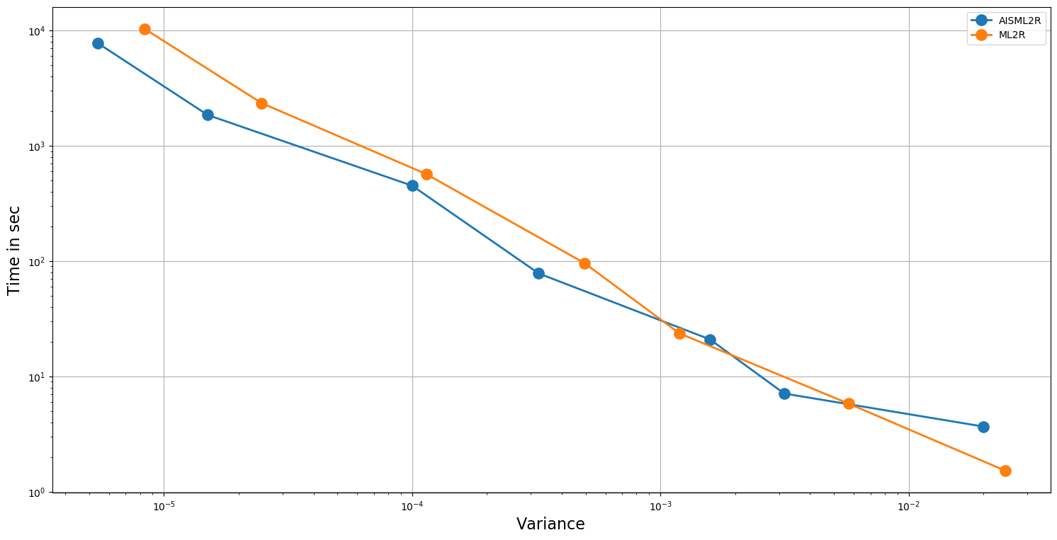
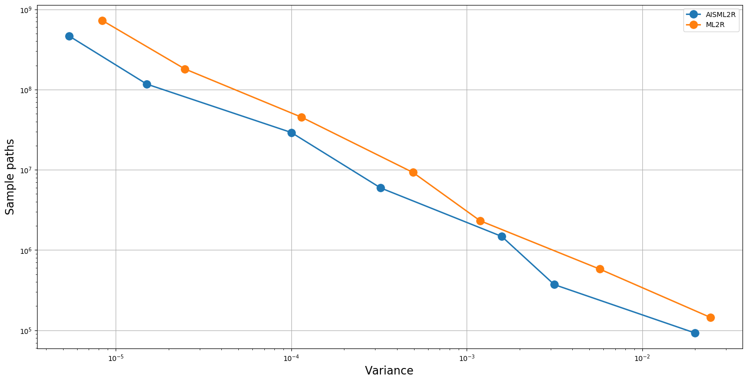
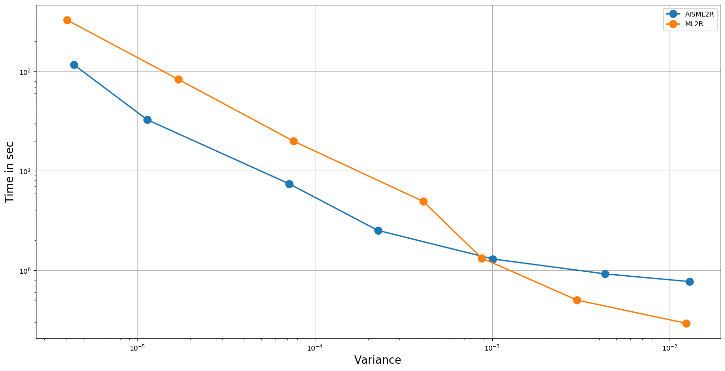
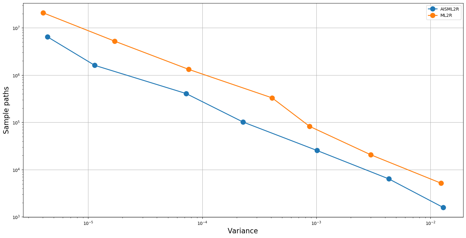
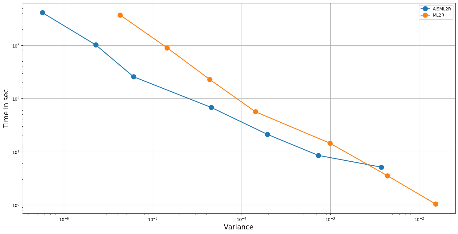
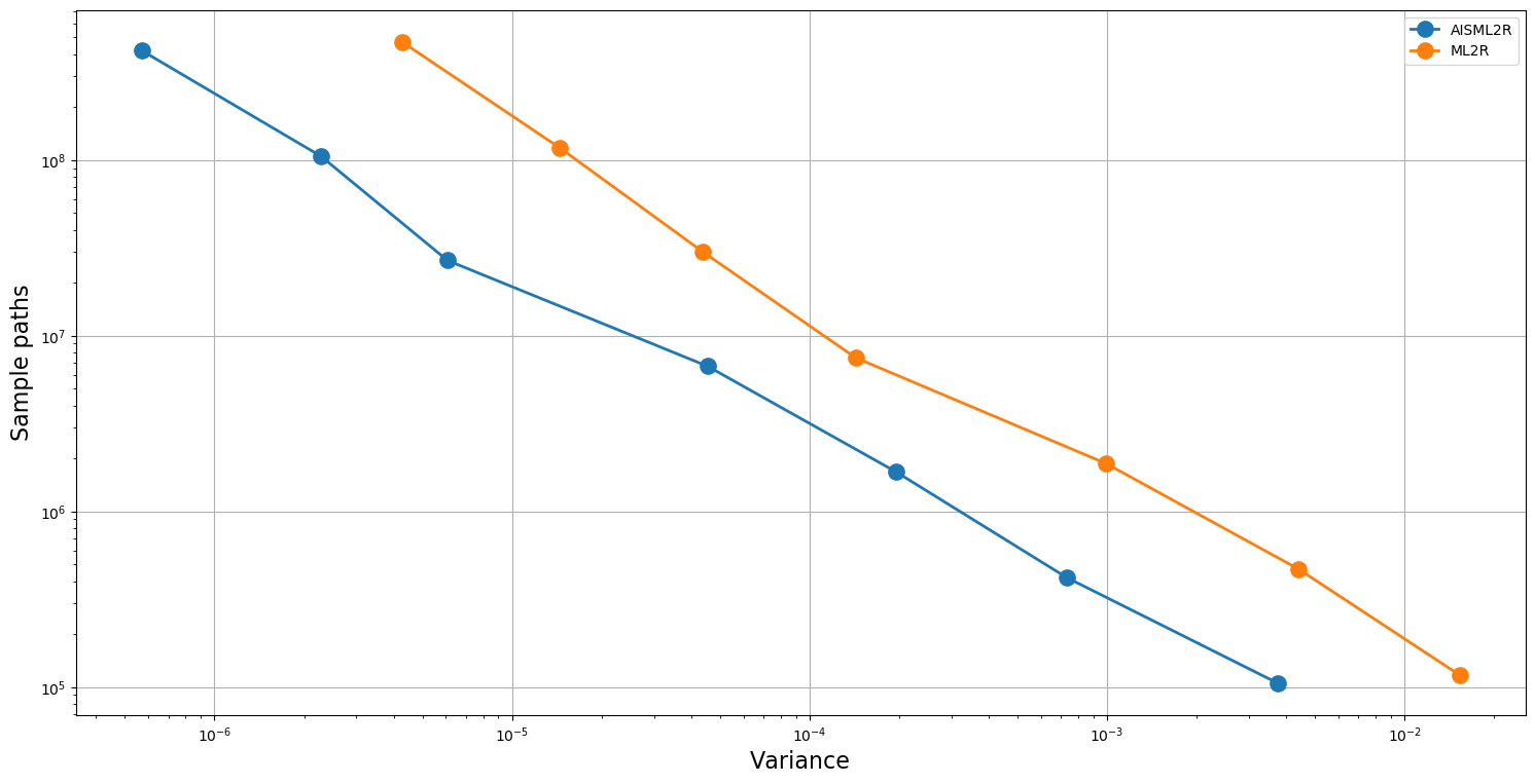
Table 3 and Table 4 demonstrate potency of the AISML2R over ML2R, under Milstein and Euler discretization, respectively. Figure 1 and Figure 2 graphically represents the performance of both the estimators under Milstein and Euler schemes, respectively. It is quite evident from the tabulated results, as well as the graphical representation, that the effectiveness of the AISML2R over ML2R increases with the requirement of greater accuracy. The value of ifk\text{if}_{k} goes from if3=0.829\text{if}_{3}=0.829, for the worst case to if9=6.78\text{if}_{9}=6.78 in the best case, while simulating under the Milstein scheme. On the other hand, under the Euler scheme, the value of ifk\text{if}_{k} goes from if3=0.508\text{if}_{3}=0.508 in the best case to if8=2.09\text{if}_{8}=2.09 in the best case. These values suggest that AISML2R can achieve desired root-mean-squared error much faster as compared to ML2R.
Refer to caption
((a)) Time (y-axis, log scale) as function of variance (x-axis, log scale)
Refer to caption
((b)) Sample Paths (y-axis, log scale) as function of variance (x-axis, log scale)
Figure 1: European Call option using Milstein Scheme
AISML2R
k N variance bias rmse time
3 1.05E+05 3.75E-03 4.93E-02 6.18E-02 5.12E+00
4 4.19E+05 7.33E-04 2.21E-02 2.72E-02 8.51E+00
5 1.68E+06 1.95E-04 1.17E-02 1.43E-02 2.12E+01
6 6.70E+06 4.54E-05 5.68E-03 7.01E-03 6.81E+01
7 2.68E+07 6.07E-06 2.14E-03 2.48E-03 2.57E+02
8 1.05E+08 2.28E-06 1.14E-03 1.51E-03 1.02E+03
9 4.20E+08 5.69E-07 5.99E-04 7.55E-04 4.14E+03
ML2R
k N variance bias rmse time
3 1.17E+05 1.53E-02 1.07E-01 1.24E-01 1.04E+00
4 4.68E+05 4.41E-03 5.47E-02 6.66E-02 3.52E+00
5 1.87E+06 9.93E-04 2.60E-02 3.17E-02 1.44E+01
6 7.48E+06 1.43E-04 1.05E-02 1.26E-02 5.65E+01
7 2.99E+07 4.39E-05 5.29E-03 6.62E-03 2.28E+02
8 1.17E+08 1.45E-05 2.96E-03 3.82E-03 9.01E+02
9 4.69E+08 4.28E-06 1.61E-03 2.14E-03 3.73E+03
Table 3: Pricing European Option using Milstein Scheme
Refer to caption
((a)) Time (y-axis, log scale) as function of variance (x-axis, log scale)
Refer to caption
((b)) Sample Paths (y-axis, log scale) as function of variance (x-axis, log scale)
Figure 2: European Call option using Euler Scheme
AISML2R
k N variance bias rmse time
3 9.28E+04 1.99E-02 4.39E-02 1.48E-01 3.69E+00
4 3.71E+05 3.15E-03 1.25E-02 5.75E-02 7.12E+00
5 1.48E+06 1.58E-03 2.39E-03 3.98E-02 2.10E+01
6 5.94E+06 3.23E-04 6.25E-03 1.90E-02 7.83E+01
7 2.92E+07 9.99E-05 4.76E-04 1.00E-02 4.51E+02
8 1.17E+08 1.50E-05 6.49E-05 3.87E-03 1.85E+03
9 4.67E+08 5.40E-06 4.10E-04 2.36E-03 7.79E+03
ML2R
N variance bias rmse time
3 1.45E+05 2.44E-02 5.25E-03 1.56E-01 1.53E+00
4 5.80E+05 5.71E-03 5.18E-03 7.57E-02 5.83E+00
5 2.32E+06 1.19E-03 8.79E-03 3.55E-02 2.37E+01
6 9.28E+06 4.93E-04 2.27E-03 2.23E-02 9.64E+01
7 4.54E+07 1.14E-04 1.52E-03 1.08E-02 5.68E+02
8 1.81E+08 2.47E-05 8.38E-05 4.97E-03 2.35E+03
9 7.26E+08 8.37E-06 6.35E-04 2.96E-03 1.03E+04
Table 4: Pricing European Option using Euler Scheme

5.2 Lookback Option

In this section we consider a partial lookback call option, whose payoff is defined as,

P(XT)=erT(XTζmint[0,T]X(t))+,whereζ1.P(X_{T})=e^{-rT}(X_{T}-\zeta\min_{t\in[0,T]}X(t))_{+},\leavevmode\nobreak\ \text{where}\leavevmode\nobreak\ \zeta\geq 1. (64)

The parameters for the purpose of the practical implementation, taken from [10], are X0=100X_{0}=100, r=0.15r=0.15, σ=0.1\sigma=0.1 and T=1T=1. Also, the value of ζ\zeta is set as ζ=1.1\zeta=1.1. Further, the refinement factor MM used to perform the simulation at various level of dicretization, is set as M=8M=8, for either case. With these parameters, the price obtained through closed form solution is 𝐉0=8.89343\mathbf{J}_{0}=8.89343. The simulation is carried out using both Milstein and Euler scheme, as described above. In order to exploit the full essence of Milstein discretization, we use the formula described below in order to simulate the value of mint[0,T]X(t)\min_{t\in[0,T]}X(t) on various refinement level, [3].

Xn,minnl=12(Xnnl+Xn+1nl(Xn+1nlXnnl)22(σXnnl)2hllogUn),UnUinf(0,1).X^{n_{l}}_{n,\min}=\frac{1}{2}\left(X^{n_{l}}_{n}+X^{n_{l}}_{n+1}-\sqrt{\left(X^{n_{l}}_{n+1}-X^{n_{l}}_{n}\right)^{2}-2\left(\sigma X^{n_{l}}_{n}\right)^{2}h_{l}\log U_{n}}\right),\leavevmode\nobreak\ U_{n}\sim\text{Uinf}(0,1). (65)

Further, we set Xn,minnl1=Xn,minnlX^{n_{l-1}}_{n,\min}=X^{n_{l}}_{n,\min}. In this case we stop the stochastic algorithm after 200200 iterations for either case.

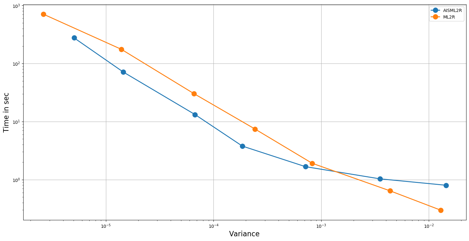
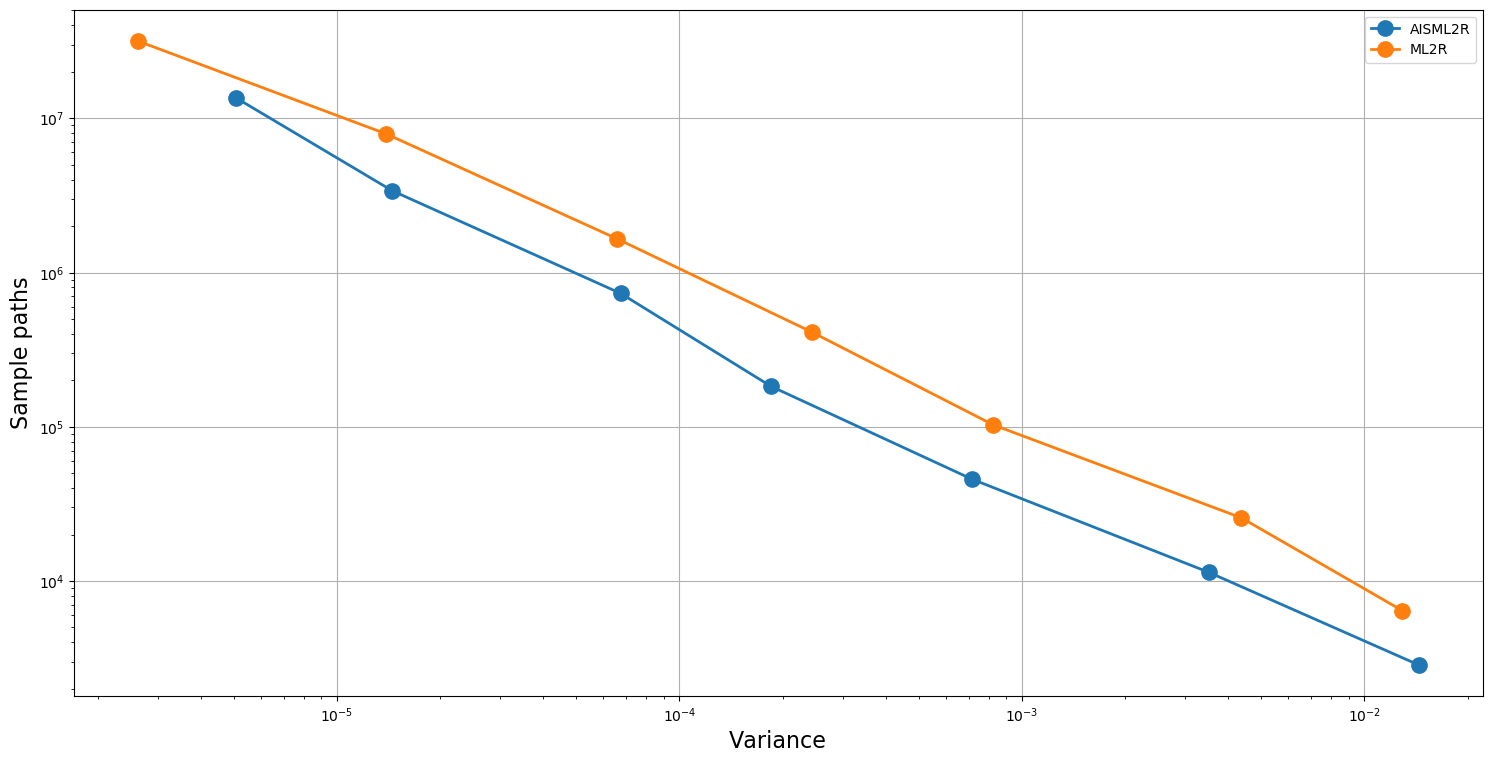
The results summarized in Table 5 and Table 6 shows the efficacy of AISML2R over ML2R in the case of both Euler and Milstein discretization scheme, respectively. Figure 3 and Figure 4 graphically represents the performance of both estimators under Milstein and Euler schemes, respectively. Similar to the case of European Option, we can easily observe that the efficiency of AISML2R over ML2R increases as more accuracy is required. The value of if goes from if3=0.365\text{if}_{3}=0.365 in the worst case to if8=3.81\text{if}_{8}=3.81 in the best case, while simulating under Milstein scheme. Under the Euler scheme, the value goes from if3=0.333\text{if}_{3}=0.333 in the worst case to if6=2.58\text{if}_{6}=2.58 in the best case.

AISML2R
k N variance bias rmse time
3 2.86E+03 1.44E-02 2.41E-02 1.22E-01 7.99E-01
4 1.14E+04 3.51E-03 2.13E-03 5.93E-02 1.03E+00
5 4.58E+04 7.14E-04 8.31E-03 2.80E-02 1.67E+00
6 1.83E+05 1.85E-04 9.92E-03 1.68E-02 3.78E+00
7 7.33E+05 6.73E-05 9.88E-03 1.28E-02 1.32E+01
8 3.39E+06 1.45E-05 8.88E-03 9.66E-03 7.14E+01
9 1.36E+07 5.06E-06 8.81E-03 9.09E-03 2.77E+02
ML2R
k N variance bias rmse time
3 6.43E+03 1.29E-02 1.45E-02 1.15E-01 2.97E-01
5 2.57E+04 4.37E-03 1.17E-03 6.61E-02 6.39E-01
5 1.03E+05 8.24E-04 1.19E-02 3.11E-02 1.91E+00
6 4.12E+05 2.43E-04 8.33E-03 1.77E-02 7.42E+00
7 1.65E+06 6.59E-05 9.35E-03 1.24E-02 3.02E+01
8 7.93E+06 1.39E-05 9.05E-03 9.79E-03 1.76E+02
9 3.17E+07 2.62E-06 9.08E-03 9.22E-03 7.10E+02
Table 5: Pricing Lookback Option using Euler Scheme
Refer to caption
((a)) Time (y-axis, log scale) as function of variance (x-axis, log scale)
Refer to caption
((b)) Sample Paths (y-axis, log scale) as function of variance (x-axis, log scale)
Figure 3: Pricing Lookback Call option using Euler Scheme
AISML2R
k N variance bias rmse time
3 1.59E+03 1.29E-02 7.52E-02 1.36E-01 7.71E-01
4 6.38E+03 4.31E-03 2.92E-02 7.19E-02 9.21E-01
5 2.55E+04 1.01E-03 2.99E-02 4.36E-02 1.30E+00
6 1.02E+05 2.27E-04 2.64E-02 3.04E-02 2.52E+00
7 4.08E+05 7.20E-05 2.43E-02 2.57E-02 7.40E+00
8 1.61E+06 1.14E-05 2.36E-02 2.38E-02 3.27E+01
9 6.44E+06 4.40E-06 2.27E-02 2.28E-02 1.17E+02
ML2R
k N variance bias rmse time
3 5.16E+03 1.24E-02 2.65E-02 1.14E-01 2.93E-01
5 2.06E+04 3.00E-03 2.76E-02 6.13E-02 5.02E-01
5 8.25E+04 8.71E-04 2.90E-02 4.14E-02 1.33E+00
6 3.30E+05 4.09E-04 2.34E-02 3.09E-02 4.93E+00
7 1.32E+06 7.61E-05 2.48E-02 2.63E-02 1.99E+01
8 5.21E+06 1.71E-05 2.39E-02 2.42E-02 8.31E+01
9 2.08E+07 4.02E-06 2.26E-02 2.27E-02 3.30E+02
Table 6: Pricing Lookback Option using Milstein Scheme
Refer to caption
((a)) Time (y-axis, log scale) as function of variance (x-axis, log scale)
Refer to caption
((b)) Sample Paths (y-axis, log scale) as function of variance(x-axis, log scale)
Figure 4: Pricing Lookback Call option using Milstein Scheme

6 Conclusion

This paper presents a novel combination of ML2R and importance sampling algorithm developed upon the studies carried out in [10, 13, 15, 21, 22]. As evident from the numerical results presented in Section 5, the adaptive estimator outperforms AISML2R whenever a high degree of accuracy is required. One of the critical features of this, presented in the paper, is the use of a higher order scheme for discretizing the underlying SDE. Therefore, accommodating the antithetic feature developed by Giles [6] to simulate higher dimensional SDEs, using the Milstein scheme, in the realm of the above-developed algorithm, can substantially affect the overall computational time. Further, the completely automated nature of the algorithm gives its edge over the already existing estimators. However, it may be pointed out that a small amount of fine-tuning may be required while dealing with the Euler discretization scheme. In this paper, besides establishing the existence and uniqueness of the optimal parameter on various levels of resolutions (Section 4.1), we have also proved the Strong Law of Large Numbers in Section 4.2, proving the convergence of the adaptive estimator to the standard expectation. However, proving the Central Limit theorem still requires further detailed study of our estimator.

References

  • [1] M. B. Giles, “Multilevel monte carlo path simulation,” Operations research, vol. 56, no. 3, pp. 607–617, 2008.
  • [2] S. Heinrich, “Multilevel monte carlo methods,” in International Conference on Large-Scale Scientific Computing, pp. 58–67, Springer, 2001.
  • [3] M. Giles, “Improved multilevel monte carlo convergence using the milstein scheme,” in Monte Carlo and Quasi-Monte Carlo Methods 2006, pp. 343–358, Springer, 2008.
  • [4] M. B. Giles, K. Debrabant, and A. Rössler, “Analysis of multilevel monte carlo path simulation using the milstein discretisation,” Discrete & Continuous Dynamical Systems-B, vol. 24, no. 8, p. 3881, 2019.
  • [5] M. Giles and L. Szpruch, “Multilevel monte carlo methods for applications in finance,” Recent Developments in Computational Finance: Foundations, Algorithms and Applications, pp. 3–47, 2013.
  • [6] M. B. Giles and L. Szpruch, “Antithetic multilevel monte carlo estimation for multidimensional sdes,” in Monte Carlo and Quasi-Monte Carlo Methods 2012, pp. 367–384, Springer, 2013.
  • [7] M. B. Giles and B. J. Waterhouse, “Multilevel quasi-monte carlo path simulation,” in Advanced financial modelling, pp. 165–182, De Gruyter, 2009.
  • [8] M. B. Giles, “Multilevel monte carlo methods,” Acta Numerica, vol. 24, pp. 259–328, 2015.
  • [9] C.-h. Rhee and P. W. Glynn, “Unbiased estimation with square root convergence for sde models,” Operations Research, vol. 63, no. 5, pp. 1026–1043, 2015.
  • [10] V. Lemaire and G. Pagès, “Multilevel richardson–romberg extrapolation,” Bernoulli, vol. 23, no. 4A, pp. 2643–2692, 2017.
  • [11] P. E. Kloeden and E. Platen, “Stochastic differential equations,” in Numerical Solution of Stochastic Differential Equations, pp. 103–160, Springer, 1992.
  • [12] D. Giorgi, V. Lemaire, and G. Pagès, “Limit theorems for weighted and regular multilevel estimators,” Monte Carlo Methods and Applications, vol. 23, no. 1, pp. 43–70, 2017.
  • [13] B. Arouna, “Adaptative monte carlo method, a variance reduction technique,” 2004.
  • [14] P. Glasserman, Monte Carlo methods in financial engineering, vol. 53. Springer, 2004.
  • [15] M. B. Alaya, K. Hajji, and A. Kebaier, “Importance sampling and statistical romberg method,” Bernoulli, vol. 21, no. 4, pp. 1947–1983, 2015.
  • [16] H.-F. Chen, L. Guo, and A.-J. Gao, “Convergence and robustness of the robbins-monro algorithm truncated at randomly varying bounds,” Stochastic Processes and their Applications, vol. 27, pp. 217–231, 1987.
  • [17] H.F.Chen and Y. Zhu, “Stochastic approximation procedures with randomly varying truncations,” Science in China, Ser. A, 1986.
  • [18] C. Andrieu, É. Moulines, and P. Priouret, “Stability of stochastic approximation under verifiable conditions,” SIAM Journal on control and optimization, vol. 44, no. 1, pp. 283–312, 2005.
  • [19] J. Lelong, “Almost sure convergence of randomly truncated stochastic algorithms under verifiable conditions,” Statistics & Probability Letters, vol. 78, no. 16, pp. 2632–2636, 2008.
  • [20] V. Lemaire and G. Pagès, “Unconstrained recursive importance sampling,” The Annals of Applied Probability, vol. 20, no. 3, pp. 1029–1067, 2010.
  • [21] M. B. Alaya, K. Hajji, and A. Kebaier, “Improved adaptive multilevel monte carlo and applications to finance,” arXiv preprint arXiv:1603.02959, 2016.
  • [22] A. Kebaier and J. Lelong, “Coupling importance sampling and multilevel monte carlo using sample average approximation,” Methodology and Computing in Applied Probability, vol. 20, no. 2, pp. 611–641, 2018.
  • [23] M. B. Alaya and A. Kebaier, “Central limit theorem for the multilevel monte carlo euler method,” The Annals of Applied Probability, vol. 25, no. 1, pp. 211–234, 2015.
  • [24] S. Laruelle, C.-A. Lehalle, et al., “Optimal posting price of limit orders: learning by trading,” Mathematics and Financial Economics, vol. 7, no. 3, pp. 359–403, 2013.
  • [25] P. Hall and C. C. Heyde, Martingale limit theory and its application. Academic press, 2014.