Currently at: ]School of Physics, The University of Sydney, Sydney, New South Wales 2006, Australia
The University of Sydney Nano Institute, The University of Sydney, NSW 2006, Australia
Multifunctional on-chip storage at telecommunication wavelength for quantum networks
Abstract
Quantum networks will enable a variety of applications, from secure communication and precision measurements to distributed quantum computing. Storing photonic qubits and controlling their frequency, bandwidth and retrieval time are important functionalities in future optical quantum networks. Here we demonstrate these functions using an ensemble of erbium ions in yttrium orthosilicate coupled to a silicon photonic resonator and controlled via on-chip electrodes. Light in the telecommunication C-band is stored, manipulated and retrieved using a dynamic atomic frequency comb protocol controlled by linear DC Stark shifts of the ion ensemble’s transition frequencies. We demonstrate memory time control in a digital fashion in increments of 50 ns, frequency shifting by more than a pulse-width ( MHz), and a bandwidth increase by a factor of three, from 6 MHz to 18 MHz. Using on-chip electrodes, electric fields as high as 3 kV/cm were achieved with a low applied bias of 5 V, making this an appealing platform for rare earth ions, which experience Stark shifts of the order of 10 kHz/(V/cm).
I Introduction
Optical quantum memories will enable long distance quantum communication using quantum repeater protocols [1, 2, 3]. A quantum memory device which can control the bandwidth and frequency of stored light is additionally useful, as it can interface between optical elements which have different optimal operating points. Erbium-doped materials are a promising solid-state platform for ensemble-based optical quantum memories because of their long-lived optical transition in the telecommunication C-band that is highly coherent at cryogenic temperatures [4, 5]. This allows for integration of memory systems with low-loss optical fibers, opening up opportunities for repeaters over continental distances, as well as integration with silicon photonics [6, 7] one of the most advanced platforms for integrated photonics. Spin transitions in 167Er3+-doped yttrium orthosilicate (167Er3+:Y2SiO5) have also been shown to have long relaxation and coherence lifetimes at cryogenic temperatures and high magnetic fields [8] which opens the possibility for long term spin wave memories.
There have been several demonstrations of optical storage in erbium-doped materials [9, 10, 11, 12, 13, 14], including storage at the quantum level [9, 10, 14], and on-chip storage [10, 14]. These results are part of a larger body of optical quantum memory research [15, 3], using rare-earth-ion-doped crystals [16, 17, 18, 19], atomic gases [20, 21], and single atoms or defects [22, 23]. In parallel with efforts to increase the efficiency [20] and storage time [19, 18] of quantum memories, several works have focused on new types of multifunctional devices [24, 25, 26] in which control fields are used to modify the state of the light during storage.
In many quantum repeater protocols [27], quantum memories act as interfaces between emitters such as quantum dots [28] or individual atoms [7]. Dynamic control of the optical pulses stored in these memories can correct for differences between individual emitters, leading to higher indistinguishably for Bell State measurements at the entanglement swapping stage of quantum repeater protocols [1]. In addition, with control over the frequency of stored light, one can map an input mode to a different output mode in a frequency multiplexed quantum memory, which enables quantum networks with fixed-time quantum memories [29].
In this work, we use a silicon resonator evanescently coupled to 167Er3+:Y2SiO5 ions and gold electrodes to realize a multifunctional on-chip device which can not only store light, but also dynamically modify its frequency and bandwidth. Electrodes create a DC electric field that can be rapidly switched, which enables control of the 167Er3+ ions’ optical transition frequency via the DC Stark shift [30]. Using a resonator increases the interaction between light and the ion ensemble, allowing on-chip implementation of the atomic frequency comb (AFC) memory protocol [31]. This protocol allows multiplexing in frequency, which offers a significant advantage in quantum repeater networks [32]. Additionally, the on-chip electrodes are patterned close together to achieve the high electric fields required for Stark shift control with CMOS compatible, applied voltages. We demonstrate dynamic control of memory time in a digital fashion, as well as modification of the frequency and bandwidth of stored light.
II Hybrid Si-167Er3+:Y2SiO5 resonator with electrodes
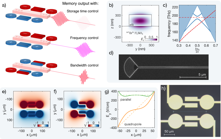
The multifunctional device consists of an optical resonator coupled to 167Er3+:Y2SiO5 ions between gold electrodes. Using the AFC quantum storage protocol [34] and the ions’ Stark shift, light can be stored and manipulated in this device. Figure 1a shows a schematic of the device and the three functionalities demonstrated in this work: memory time control, frequency control, and bandwidth control. Different electric field configurations are created by applying a positive (blue) or negative (red) bias to each electrode. For the true device dimensions, see the micrograph in Fig. 1h.
The optical resonator used in this work is a Fabry-Perot resonator comprised of a 100 m amorphous silicon (Si) waveguide on 167Er3+:Y2SiO5 with photonic crystal mirrors on either end. Figures 1b-d show simulations and micrographs of this resonator. The waveguide is nm tall and nm wide. Ten percent of the energy of the transverse-magnetic optical waveguide mode penetrates into the 167Er3+:Y2SiO5 and evanescently couples to the 167Er3+ ions. Photonic crystal mirrors on either side are formed by a repeating pattern of elliptical air holes in the Si waveguide with period nm. A grating coupler is used to couple light from a free-space mode into and out of the resonator. The amorphous silicon resonator is fabricated on top of an 167Er3+:Y2SiO5 chip using a deposition and etching process similar to Ref. [6]. The 167Er3+:Y2SiO5 substrate is doped with isotopically purified 167Er3+ ions at 135 ppm, measured by secondary ion mass spectrometry, and cut perpendicular to the crystal axis, such that the electric field of the transversal magnetic (TM) optical mode is polarized along this axis.
Quality factors of up to were measured for weakly coupled resonators, where the photonic crystal mirrors on both sides were designed to be highly reflective. The device used in this work is made one-sided for more efficient quantum storage [34, 14] by using fewer photonic crystal periods in one mirror to make it less reflective. Light is sent into and measured from the side with the lower reflectivity mirror. The intrinsic quality factor for this device is also lower than the weakly coupled resonators, leading to a quality factor of and a coupling ratio of , where is the coupling rate through the lower reflectivity mirror and is the total decay rate [35].
Electrodes are used to apply electric fields to those ions coupled to the optical resonator. There are four independently biased gold electrodes, each comprised of a 70 m diameter circle connected to a rectangle. They are patterned onto the 167Er3+:Y2SiO5 after the Si resonators using electron-beam lithography followed by electron-beam gold evaporation and lift-off. Figures 1e-g show simulations of the two electrode biasing configurations: parallel, which applies a nearly constant electric field to all ions (), and quadrupole, which applies an electric field gradient along the resonator (approximating ), where and are constants. The electrode geometry was designed to best approximate these two electric field profiles with four independently biased electrodes, while providing a large electric field for a given applied bias (). In the 167Er3+:Y2SiO5 region where ions are coupled to the optical mode, the component of the electric field is dominant (), and it does not vary significantly in the and directions. Therefore only , which is aligned to the -axis of the Y2SiO5 crystal, is considered.
The device is thermally connected to the coldest plate of a dilution refrigerator, the temperature of which is mK. A static magnetic field of 0.98 T is applied along the Y2SiO5 -axis with a superconducting electromagnet. Trim coils are used to cancel any magnetic field component along the -axis. The remainder of the measurement setup was similar to the one described in Ref. [14].
III DC Stark shift in 167Er3+:Y2SiO5
Er3+:Y2SiO5 has been extensively studied for quantum applications [4, 5, 36, 11, 12, 13, 7, 14, 37], including demonstrations of AFC storage [11, 12, 14]. Erbium ions substitute for yttrium ions in Y2SiO5 in 2 crystallographic sites, each of which has four different orientations due to the crystal symmetry [38]. In this work, we use crystallographic site 2, which has an optical transition near nm [4]. 167Er3+ has a nuclear spin , which together with an effective electron spin, leads to 16 hyperfine levels in both the optical ground and excited states. At high fields and low temperatures, the lowest 8 ground-state hyperfine levels are long-lived [8, 14], enabling the spectral holeburning that is required to create atomic frequency combs.
Dynamic control is enabled by the DC Stark shift. When a rare earth ion in a crystal interacts with a DC electric field , its optical transition frequency is shifted due to the difference between the permanent electric dipole moments in the optical excited and optical ground states . For non-centrosymmetric sites such as the yttrium sites in Y2SiO5 for which Er3+ ions substitute, the linear Stark shift term dominates, where is the local field correction tensor [30].
The Stark shift is dependent on the orientation of the applied field relative to [39]. Without knowing or , the Stark shift can be empirically characterized for an electric field applied in a particular direction using the Stark shift parameter given . We measured kHz/(V/cm) for nominally aligned with the Y2SiO5 crystal -axis (see Appendix A).
In an ensemble of 167Er3+:Y2SiO5 ions, four different Stark shifts will be observed for an arbitrary electric field due to the four orientations of each crystallographic site [38]. For electric fields parallel or perpendicular to the -axis, the Stark shifts of the four subclasses are pair-wise degenerate, resulting in two equal and opposite Stark shifts . In this work, all electric fields are applied parallel to the -axis, so we will simply refer to two 167Er3+ subclasses.
IV Atomic frequency comb storage with dynamic memory time control
After a photon is absorbed by an ensemble of ions, the ensemble of ions is described by a Dicke state [34]:
| (1) |
Each ion has a different transition frequency and position . For AFC storage, the transition frequencies form a frequency comb with period . When a photon is absorbed at , the ensemble of ions first dephase then rephase every , , leading to a coherent re-emission of the light [34]. A Stark shift enables dynamic control of light stored in the AFC by changing the optical transition frequencies of the ions. can be varied over time by changing the amplitude of the applied electric field (slowly relative to optical frequencies). This enables two types of control: electric field pulses applied between the absorption and emission of light modify the phase of the output, while electric field pulses applied during emission of light modify the frequency profile of the output light.
To achieve dynamic control of storage time, the electrodes are biased in a parallel configuration as shown in the top panel of Figure 1a. When an electric pulse is applied, the two 167Er3+:Y2SiO5 subclasses experience equal and opposite frequency shifts, . By appropriately choosing the length in time and amplitude of the electric pulse, a phase difference between subclasses can be introduced , which will prevent any coherent emission from the ensemble. An equal and opposite electric pulse can then rephase the two subclasses, and allows coherent re-emissions from the AFC. This procedure of dephasing and rephasing the ensemble works even if the electric field distribution is not perfectly homogeneous, as shown in the context of Stark Echo Modulation Memory in Reference [40]. Recently, dynamic control of memory time in AFC was demonstrated using this same procedure in Pr3+:Y2SiO5 [41]. Reference [12] proposed a similar protocol but using an electric field gradient.
The pulse sequence used to achieve dynamic control of AFC storage is shown in Figure 2a. Not shown is the initialization to move most of the population into one hyperfine state, which is performed before every experiment [14, 8]. First, an AFC with period is created by repeatedly burning away population between the teeth of the comb, times. Then, an input pulse indicated by the red laser pulse is sent into the resonator at and is absorbed by the AFC. Shown in light red are possible emissions corresponding to rephasing events of the AFC at times . Without electric field control, the output of the memory (the first and largest emission), would be centered at (). The schematic shows instead an emission in red at (), obtained when a first electric pulse is applied before the first emission and a compensating pulse is applied immediately before the third emission.
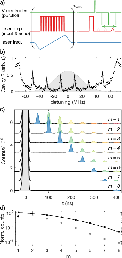
Figure 2b shows the AFC used in this experiment. The period of the comb, extracted from the fit, is MHz, which corresponds to a minimum storage time of ns. Figure 2c shows dynamically controlled storage for various values of . Two electric pulses were used to control memory time. The first was a 10 ns long pulse with amplitude 2.0 kV/cm centered at ns. The second was 10 ns long with an opposite amplitude of -2.0 kV/cm, and its center position was varied as ns ns to allow the emission at . For the case, no electric pulses were applied. Between the two electric pulses, emission was suppressed down to the dark counts level, a factor of 100 lower than peak emission counts. The presence of multiple smaller pulses following the output pulse is a feature of the high finesse and low efficiency of the memory (see Appendix B). For higher efficiency, high finesse AFCs, subsequent emissions are significantly suppressed [41].
Figure 2d shows the energy emitted in the time bin for . The data is fit to the dephasing term in the theoretical storage efficiency for a comb with Gaussian teeth: [34, 12], where is the comb finesse, and is the full-width at half maximum (FWHM) of each tooth. The data point is excluded from the fit because the approximately 100 ns dead time of the single photon detector after the input pulse is thought to lead to undercounting in that time bin. A comb finesse of ( MHz) is extracted from this fit. This corresponds to a point of 240 ns ( for digital storage time). To improve on this scaling requires a smaller tooth width . The grey data in Fig. 2d show the total counts in the time bin when the previous output pulses are not suppressed.
V Dynamic frequency control
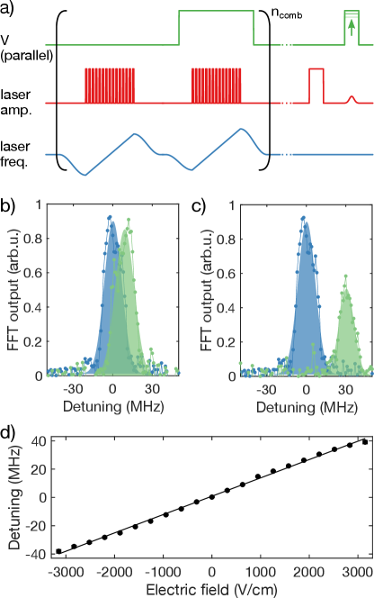
The frequency of light stored in an AFC can be dynamically modified during emission. The atomic frequency comb is shifted in frequency during the emission of stored light by biasing the electrodes in the parallel configuration as shown in the middle panel of Figure 1a. The pulse sequence used to achieve AFC storage with frequency control is shown in Figure 3a. The first step is to eliminate one of the two 167Er3+ subclasses from the spectral window, leaving only ions which experience a positive Stark shift, (the choice of subclass is arbitrary). This is accomplished using a two-part comb burning procedure. With the first burning step, a normal AFC containing both subclasses is created using a sequence of laser pulses. For the second burning step, the two subclasses are split by using a parallel electric field, and a similar sequence of laser pulses is used, but with a frequency shift of . This burns away ions with a negative shift .
Repeating the comb burning procedure times, an AFC with width 145 MHz, and a period MHz is created. An input pulse is sent in and the rephasing of the AFC causes an emission at ns. During this emission, an electric field pulse with amplitude applied in the parallel configuration will cause the ions to emit with a frequency shift of . Figures 3b-c show the light emitted from the memory, with and without a frequency shift. A heterodyne measurement is used to measure the frequency of the output pulse directly. Figure 3d shows the linear frequency shift as a function of electric field. The decrease in output amplitude with frequency shift evident in Figures 3b-c is mainly due to the inhomogeneity of Stark shifts experienced by the ions (see Appendix A).
VI Dynamic bandwidth control
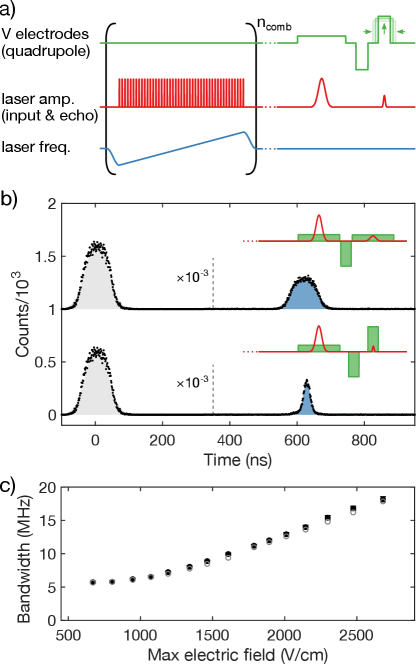
The bandwidth of stored light can be dynamically controlled by biasing the electrodes in a quadrupole configuration as shown in the bottom panel of Figure 1a. Figure 4a shows the pulse sequence used to achieve AFC storage with bandwidth control. First, an AFC with MHz and bandwidth 144 MHz is created by repeatedly burning away population times. Next, an input pulse is sent into the device, leading to an output pulse at ns. In the quadrupole configuration, electric pulses create a gradient electric field across the ions so that each ion experiences a different Stark shift. Electric pulses are applied during the input and output optical pulses, and also during the wait time. The first electric field pulse, applied during the absorption of the input pulse, and the third electric field pulse, applied during the emission of stored light, induce changes to the atomic frequency comb which lead to a change in the output light frequency profile. The second pulse during the wait time is used to add phase compensation, accounting for the fact that AFC storage is first-in-first-out [42, 24].
Figure 4b shows AFC storage with no broadening (top) and with the maximum achieved bandwidth broadening (bottom). A broadening in frequency space is seen as a narrowing of the output pulse in time. By fitting the output pulses to Gaussians, the temporal FWHMs () of input and output pulses are extracted and converted to bandwidth or frequency FWHMs () using: . Figure 4c shows the trend of output bandwidth as a function of the maximum electric field applied during the third pulse (the electric field across the resonator ranges from to ). To confirm that the trend observed in the data is expected given the atomic frequency comb profile, the input pulse, and the electric field distribution , a simulation of the experiment was performed by numerically integrating the time-evolution equations of the atoms and cavity (see Appendix C). The simulation data reproduces the trend in FWHM as a function of field. The only previously unknown parameter used in this simulation was the distance that the optical mode penetrates into the photonic crystal mirrors, which modifies the effective resonator length and changes the value of . This parameter was found to be m for each mirror by coarsely sweeping in 1 m increments in the simulation to find the best fit to the data.
VII Discussion
In this work, we have demonstrated the capabilities of an on-chip optical storage device with DC Stark shift control. Taking this technology on-chip has two main advantages. First, it allows miniaturization and future integration with other optical components on chip. Second, it enables simple generation of large electric fields. Because the distance between electrodes across the resonator is small (a minimum of 20 m), electric fields of kV/cm are generated with just V of applied bias in the parallel configuration. Such biases were easily supplied by a function generator with no additional amplification. In the quadrupole configuration, electric field gradients of up to 50 V/cm/m were generated, corresponding to gradient of 0.58 MHz/m in 167Er3+:Y2SiO5 transition frequencies.
For the dynamically controlled memory times in Fig. 2d, an excellent match was found between the amplitude of stored light as a function of time and the theoretical limit due to the dephasing of a comb with finesse , indicating that the two electric field control pulses did not introduce any irreversible dephasing. This was also confirmed using a two pulse photon echo measurement, where inserting two equal and opposite electric field pulses between the first and second optical pulses was found not to decrease the optical coherence time , which was measured in this device to be s.
Frequency control was demonstrated for up to MHz. In this work, the maximum shift was set by the maximum applied electric field of kV/cm. One technical difficulty is that ions from the other subclass that are outside of the comb will act as an absorbing background when the comb is shifted in frequency and the other subclass experiences an opposite frequency shift. Assuming that the comb can be sufficiently separated in frequency from the other subclass using high electric fields, a more fundamental limit is set by the inhomogeneity of the Stark shifts, which leads to a decrease in storage efficiency with increasing frequency shift. In this device, the Stark shift inhomogeneity was dominated by an electric field distribution that was not perfectly homogeneous (see Fig. 1g). Even in a perfectly homogeneous field, however, some inhomogeneity in Stark shifts will exist due to crystal field variations throughout the crystal [30].
The bandwidth of stored light was changed by a factor of three from 6 MHz to 18 MHz. The maximum broadening in this case was limited by the maximum electric field gradient of 50 V/cm/m. With higher gradients, stored pulses could be broadened up to half the value of the bandwidth of the comb, and the bandwidth of combs in this material is limited to MHz [14]. Decreasing the bandwidth of a stored pulse is not possible with this procedure, because the AFC cannot be made narrower with a gradient electric field, only wider. Narrowing the AFC could be accomplished with a frequency selective shift such as the AC Stark shift. Note that while digital memory time and frequency control theoretically do not affect the storage efficiency, the bandwidth control procedure has some associated loss. This is because the AFC rephasing does not always finish within the window defined by the third electric pulse, so the edges of the emitted pulse’s temporal envelope are clipped.
An on-chip resonator allows for storage efficiencies approaching unity if the impedance matching condition is met [31]. In this device, the storage efficiency was up to , depending on the finesse of the comb created, and was mainly limited by the low coupling between the ensemble of ions and the optical mode of the resonator, characterized by an ensemble cooperativity . The storage time on an optical transition is ultimately limited by the optical coherence time . However, in 167Er3+:Y2SiO5, superhyperfine coupling to yttrium nuclear spins in the crystal prevents the creation of narrow spectral features, which means a low storage efficiency for storage times longer than ns [14]. Superhyperfine coupling is a major limitation to high-efficiency long lived storage in 167Er3+:Y2SiO5 when using memory protocols based on spectral tailoring such as AFC.
For quantum repeater applications, the duration and efficiency of on-chip storage must be improved. Improvements to the intrinsic quality factor of the resonator are required to reach the impedance matching condition. Creative solutions such as using clock transitions in 167Er3+:Y2SiO5[43, 44, 37], which are less sensitive to superhyperfine coupling, or finding new crystal hosts for erbium ions [45] can be used to overcome the superhyperfine limit. Another requirement of quantum memories is to store quantum states of light with high fidelity. This has already been demonstrated with the AFC protocol [9]. Storage of weak coherent states using the AFC protocol with DC Stark shift control of storage time has also been recently demonstrated [41]. Future work should include demonstrations of on-chip storage of light at the quantum level with dynamic frequency and bandwidth control. More generally, this type of device could work with different absorbers that experience linear Stark shifts, or with other quantum storage protocols that do not require spectral tailoring such as Stark echo modulation memory [40].
The functionality of the device is not limited to the demonstrations in this work. For example, a gradient field could be used instead of a homogeneous field to dynamically control the storage time. The bandwidth or frequency of emissions at any time could be modified, frequency and bandwidth control could be combined, and the order of two pulses could be reversed. A device which enables Stark shift control of an ion’s transition frequency is useful for other technologies as well. For example, a gradient electric field could be used to tune two 167Er3+ ions coupled to the same resonator into resonance with one another. This would enable entangling gates between the two ions, a key step in quantum repeater protocols using single ions [46].
VIII Conclusion
In this work we demonstrated a multifunctional on-chip device that can store light while dynamically modifying its storage time, frequency and bandwidth. Dynamic control of the memory time and the frequency profile of the output light was achieved via the linear DC stark shift of 167Er3+ ions in Y2SiO5 . We demonstrated dynamic control of memory time in a digital fashion with storage times that were multiples of ns, for up to ns. The frequency of stored light was changed by up to MHz, and the bandwidth of stored light was increased by up to a factor of three, from 6 MHz to 18 MHz. This on-chip platform, comprising a resonator evanescently coupled to an ensemble of atoms that experience a DC Stark shift and on-chip electrodes, can be adapted to other materials and other quantum memory protocols.
Acknowledgements.
We acknowledge Phillip Jahelka for help with measuring the refractive index of amorphous silicon, Yunbin Guan for help measuring the erbium concentration, and Andrei Ruskuc and Hirsh Kamakari for building the superconducting magnets for this experiment. This work was supported by Air Force Office of Scientific Research (AFOSR) Grant No. FA9550-18-1-0374, and the National Science Foundation (Grant No. EFRI 1741707). I.C. and J.R. acknowledge support from the Natural Sciences and Engineering Research Council of Canada (Grants No. PGSD2-502755- 2017 and No. PGSD3-502844-2017). J.G.B. acknowledges support of the American Australian Association’s Northrop Grumman Fellowship.Appendix A DC Stark Shift Measurement
The Stark shift parameter for electric fields applied along the Y2SiO5 crystal -axis was estimated in the same device using spectral holeburning with electrodes biased in the parallel configuration (see Fig. 1e). A comb consisting of four narrow teeth 27.5 MHz apart was created in the 167Er3+:Y2SiO5 optical transition. The frequency profile of the transition was then measured while a variable electric field was applied, which led to a field-dependent twofold splitting of each tooth, as shown in Figure 5a. This splitting results from the equal and opposite Stark shifts experienced by the two subclasses of 167Er3+:Y2SiO5 ions . Figure 5b shows the observed splitting as a function of electric field. The slope of the straight-line fit is , from which kHz/(V/cm) is extracted. This uncertainty does not take into account any misalignment between the electric field and the -axis. To align to the -axis, the device coordinate axes ( and ) were visually aligned to the Y2SiO5 chip edges ( and crystal axes), with an estimated error of .
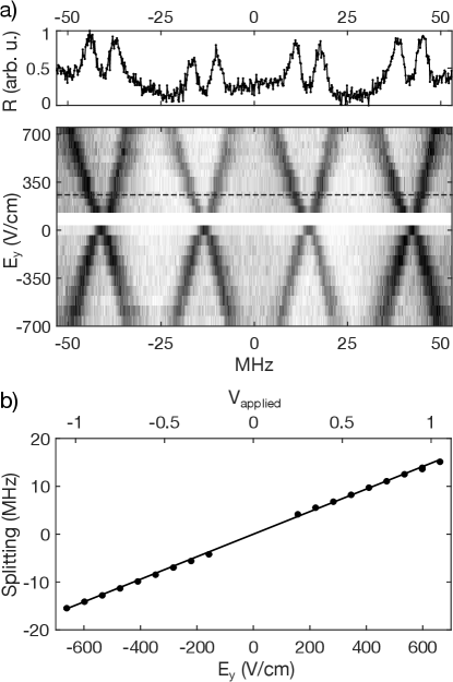
Figure 5a also shows a slight broadening of the teeth as a function of electric field. This broadening is caused by the deviation of the electric field profile from a perfectly uniform field (see Fig. 1e) and an additional measured inhomogeneity in the Stark shifts. To quantify these effects, the expected broadening was simulated by considering the optical frequencies of a large number of ions sampled from a comb tooth, with each ion experiencing an electric field sampled from the distribution in Fig. 1e, and a slightly different Stark shift parameter sampled from a Gaussian distribution with FWHM . After accounting for the known electric field inhomogeneity, we estimated the additional inhomogeneity to be characterized by kHz/(V/cm). The additional broadening could be the result of inhomogeneity in the Stark shift parameters [30] and some additional electric field inhomogeneity unaccounted for in simulation. The latter could be caused by fabrication imperfections or stray fields from other devices on the chip.
Appendix B Amplitude of the th light emission
The following section expands upon the analysis by Afzelius et al. in References [34, 31] to consider multiple emissions. An ensemble of ions is coupled to a cavity with field decay rate . An AFC is created in this ensemble of ions, which leads ion distribution to be , where , and is the number of ions. Each ion has a detuning relative to cavity center frequency, coherent decay rate , and ion-cavity coupling rate . After sending a photon into the cavity that is resonant with it, the dynamic equations [31, 47] of cavity field and atomic polarization in the rotating frame of photon frequency are
| (2) |
| (3) |
The input output formalism gives
| (4) |
where is the cavity decay rate to the input channel. We can solve Eq. (3) and get
| (5) |
Then, inserting Eq. (5) into Eq. (2), we find
| (6) | ||||
where is the Fourier transform of [34].
We have an atomic frequency comb with period , and each tooth has a shape described by , so can be written as
| (7) | ||||
The Fourier transform of is :
| (8) | ||||
Inserting Eq. (8) into Eq. (6), we find
| (9) | ||||
where is the absorption rate of atomic frequency comb[14], and .
Consider the time after the ensemble of ions absorb the light (). There are no input pulses after , so . Applying adiabatic elimination of the cavity mode () leads to
| (10) |
The cavity field at time goes as
| (11) |
From this, we can see that the amplitude of the cavity field at time is determined by the cavity field at all earlier times , where . We can theoretically find the amplitude of the cavity field at any time, which depends on how we modulate the cavity field at previous times. In our case, is much smaller than the teeth width [14], so we can ignore the term . We assume each tooth has Gaussian shape, which gives
| (12) | ||||
where is the FWHM of the Gaussian peak, and as we defined in the main text, Eq. (11) becomes
| (13) |
We also know from Eq. (4) that the amplitude of the emission (for ) is
| (14) |
At time we have
| (15) |
From the above three equations, the emission at time has the following amplitude
| (16) | ||||
The emission is the sum of to emission and the input. In the case where we don’t apply electric fields to prevent any emissions, the first and second emitted field amplitudes are
| (17) |
| (18) |
As Eq. (18) shows, the amplitude of the second emission is composed of two parts. The first part is from the light absorbed at , and the second part is from the light reabsorbed at the first emission time . The competition between these two terms determines the amplitude and the phase of the output at . When we operate in the high finesse regime (since we always want the dephasing term to be close to 1), if the amplitude of the first output is small, the amplitude of the second output will be dominated by the first term in Eq. (18), so it will still have an observable amplitude. If the amplitude of the first output is high, the amplitude of the second output will be small due to the minus sign between the two terms in Eq. (18). In particular, when the impedance matching condition[31] holds where , the second emission will be zero. This trend also holds for higher order emissions, as can be seen by extending the analysis of Eq. (16.
In the case where we apply an electric field to kill all the lower order emissions (from 1 to ), we find the output amplitude to be
| (19) |
Then, we can find the efficiency of the output pulse to be
| (20) | ||||
Appendix C Time evolution simulations
Simulations of the cavity-ion system were performed to confirm the trends observed in the bandwidth control experiment. These simulations involved numerically solving the discrete form of Eq. (2) and Eq. (3) for the cavity field and the atomic polarization of a number of ions in the rotating frame, following Reference [48]:
| (21) |
| (22) |
where is the cavity detuning and is the detuning of each ion, which can vary in time as a function of applied electric field at the location of the ion . is the detuning of each ion in the absence of an applied electric field and the sign depends on which subclass the ion is in. The cavity field is coupled to external fields as described by input-output formalism (see Equation 4). The initial conditions are , .
For the simulation, a system of differential equations (Equations 22 and 21) are numerically solved. To keep the number of equations to a reasonable size, the number of ions simulated is significantly smaller than the true number of ions coupled to the cavity . To accurately represent the strength of the interaction between the ion ensemble and the cavity, in the simulation is chosen such that , where GHz is measured from the cavity reflectance curve [14]. The time-independent frequency distribution of the ions (frequency comb) is described as a continuous distribution, and values of are sampled from it. A time dependent scalar representing the Stark shift is added to all ion detunings. for each ion is given by randomly sampling the -position along the resonator, and obtaining the corresponding electric field from Figure 1g, then varying it in amplitude and time to represent each electric pulse.
Using this simulation, the output pulse profile can be computed given , the input pulse profile centered around , and certain set of electric field control pulses.
References
- Briegel et al. [1998] H.-J. Briegel, W. Dür, J. I. Cirac, and P. Zoller, Quantum repeaters: The role of imperfect local operations in quantum communication, Phys. Rev. Lett. 81, 5932 (1998).
- Kimble [2008] H. J. Kimble, The quantum internet, Nature 453, 1023 (2008).
- Heshami et al. [2016] K. Heshami, D. G. England, P. C. Humphreys, P. J. Bustard, V. M. Acosta, J. Nunn, and B. J. Sussman, Quantum memories: Emerging applications and recent advances, J. Mod. Opt. 63, 2005 (2016).
- Böttger et al. [2006] T. Böttger, Y. Sun, C. W. Thiel, and R. L. Cone, Spectroscopy and dynamics of Er3+:Y2SiO5 at , Phys. Rev. B 74, 075107 (2006).
- Böttger et al. [2009] T. Böttger, C. W. Thiel, R. L. Cone, and Y. Sun, Effects of magnetic field orientation on optical decoherence in Er3+:Y2SiO5, Phys. Rev. B 79, 115104 (2009).
- Miyazono et al. [2017] E. Miyazono, I. Craiciu, A. Arbabi, T. Zhong, and A. Faraon, Coupling erbium dopants in yttrium orthosilicate to silicon photonic resonators and waveguides, Opt. Express 25, 2863 (2017).
- Dibos et al. [2018] A. M. Dibos, M. Raha, C. M. Phenicie, and J. D. Thompson, Atomic source of single photons in the telecom band, Phys. Rev. Lett. 120, 243601 (2018).
- Rančić et al. [2018] M. Rančić, M. P. Hedges, R. L. Ahlefeldt, and M. J. Sellars, Coherence time of over a second in a telecom-compatible quantum memory storage material, Nat. Phys. 14, 50 (2018).
- Saglamyurek et al. [2015] E. Saglamyurek, J. Jin, V. B. Verma, M. D. Shaw, F. Marsili, S. W. Nam, D. Oblak, and W. Tittel, Quantum storage of entangled telecom-wavelength photons in an erbium-doped optical fibre, Nat. Photonics 9, 83 (2015).
- Askarani et al. [2019] M. F. Askarani, M. G. Puigibert, T. Lutz, V. B. Verma, M. D. Shaw, S. W. Nam, N. Sinclair, D. Oblak, and W. Tittel, Storage and reemission of heralded telecommunication-wavelength photons using a crystal waveguide, Phys. Rev. Appl. 11, 054056 (2019).
- Lauritzen et al. [2010] B. Lauritzen, J. Minář, H. de Riedmatten, M. Afzelius, N. Sangouard, C. Simon, and N. Gisin, Telecommunication-wavelength solid-state memory at the single photon level, Phys. Rev. Lett. 104, 080502 (2010).
- Lauritzen et al. [2011] B. Lauritzen, J. Minář, H. de Riedmatten, M. Afzelius, and N. Gisin, Approaches for a quantum memory at telecommunication wavelengths, Phys. Rev. A 83, 012318 (2011).
- Dajczgewand et al. [2014] J. Dajczgewand, J.-L. L. Gouët, A. Louchet-Chauvet, and T. Chanelière, Large efficiency at telecom wavelength for optical quantum memories, Opt. Lett. 39, 2711 (2014).
- Craiciu et al. [2019] I. Craiciu, M. Lei, J. Rochman, J. M. Kindem, J. G. Bartholomew, E. Miyazono, T. Zhong, N. Sinclair, and A. Faraon, Nanophotonic quantum storage at telecommunication wavelength, Phys. Rev. Appl. 12, 024062 (2019).
- Brennen et al. [2015] G. Brennen, E. Giacobino, and C. Simon, Focus on quantum memory, New J. Phys. 17, 050201 (2015).
- Hedges et al. [2010] M. P. Hedges, J. J. Longdell, Y. Li, and M. J. Sellars, Efficient quantum memory for light, Nature 465, 1052 (2010).
- Schraft et al. [2016] D. Schraft, M. Hain, N. Lorenz, and T. Halfmann, Stopped light at high storage efficiency in a : crystal, Phys. Rev. Lett. 116, 073602 (2016).
- Holzäpfel et al. [2020] A. Holzäpfel, J. Etesse, K. T. Kaczmarek, A. Tiranov, N. Gisin, and M. Afzelius, Optical storage for 0.53 s in a solid-state atomic frequency comb memory using dynamical decoupling, New J. Phys. 22, 063009 (2020).
- Heinze et al. [2013] G. Heinze, C. Hubrich, and T. Halfmann, Stopped light and image storage by electromagnetically induced transparency up to the regime of one minute, Phys. Rev. Lett. 111, 033601 (2013).
- Hsiao et al. [2018] Y.-F. Hsiao, P.-J. Tsai, H.-S. Chen, S.-X. Lin, C.-C. Hung, C.-H. Lee, Y.-H. Chen, Y.-F. Chen, I. A. Yu, and Y.-C. Chen, Highly efficient coherent optical memory based on electromagnetically induced transparency, Phys. Rev. Lett. 120, 183602 (2018).
- Wang et al. [2019a] Y. Wang, J. Li, S. Zhang, K. Su, Y. Zhou, K. Liao, S. Du, H. Yan, and S.-L. Zhu, Efficient quantum memory for single-photon polarization qubits, Nat. Photonics 13, 346 (2019a).
- Specht et al. [2011] H. P. Specht, C. Nölleke, A. Reiserer, M. Uphoff, E. Figueroa, S. Ritter, and G. Rempe, A single-atom quantum memory, Nature 473, 190 (2011).
- Bhaskar et al. [2020] M. K. Bhaskar, R. Riedinger, B. Machielse, D. S. Levonian, C. T. Nguyen, E. N. Knall, H. Park, D. Englund, M. Lončar, D. D. Sukachev, and M. D. Lukin, Experimental demonstration of memory-enhanced quantum communication, Nature 580, 60 (2020).
- Hosseini et al. [2009] M. Hosseini, B. M. Sparkes, G. Hétet, J. J. Longdell, P. K. Lam, and B. C. Buchler, Coherent optical pulse sequencer for quantum applications, Nature 461, 241 (2009).
- Fisher et al. [2016] K. A. G. Fisher, D. G. England, J.-P. W. MacLean, P. J. Bustard, K. J. Resch, and B. J. Sussman, Frequency and bandwidth conversion of single photons in a room-temperature diamond quantum memory, Nat. Commun. 7, 11200 (2016).
- Mazelanik et al. [2019] M. Mazelanik, M. Parniak, A. Leszczyński, M. Lipka, and W. Wasilewski, Coherent spin-wave processor of stored optical pulses, NPJ Quantum Inf. 5, 22 (2019).
- Wu et al. [2020] Y. Wu, J. Liu, and C. Simon, Near-term performance of quantum repeaters with imperfect ensemble-based quantum memories, Phys. Rev. A 101, 042301 (2020).
- Wang et al. [2019b] H. Wang, H. Hu, T.-H. Chung, J. Qin, X. Yang, J.-P. Li, R.-Z. Liu, H.-S. Zhong, Y.-M. He, X. Ding, Y.-H. Deng, Q. Dai, Y.-H. Huo, S. Höfling, C.-Y. Lu, and J.-W. Pan, On-demand semiconductor source of entangled photons which simultaneously has high fidelity, efficiency, and indistinguishability, Phys. Rev. Lett. 122, 113602 (2019b).
- Sinclair et al. [2014] N. Sinclair, E. Saglamyurek, H. Mallahzadeh, J. A. Slater, M. George, R. Ricken, M. P. Hedges, D. Oblak, C. Simon, W. Sohler, and W. Tittel, Spectral multiplexing for scalable quantum photonics using an atomic frequency comb quantum memory and feed-forward control, Phys. Rev. Lett. 113, 053603 (2014).
- Macfarlane [2007] R. M. Macfarlane, Optical stark spectroscopy of solids, J. Lumin. 125, 156 (2007), festschrift in Honor of Academician Alexander A. Kaplyanskii.
- Afzelius and Simon [2010] M. Afzelius and C. Simon, Impedance-matched cavity quantum memory, Phys. Rev. A 82, 022310 (2010).
- Simon et al. [2007] C. Simon, H. de Riedmatten, M. Afzelius, N. Sangouard, H. Zbinden, and N. Gisin, Quantum repeaters with photon pair sources and multimode memories, Phys. Rev. Lett. 98, 190503 (2007).
- Deotare et al. [2009] P. B. Deotare, M. W. McCutcheon, I. W. Frank, M. Khan, and M. Loncar, High quality factor photonic crystal nanobeam cavities, Appl. Phys. Lett. 94, 121106 (2009).
- Afzelius et al. [2009] M. Afzelius, C. Simon, H. de Riedmatten, and N. Gisin, Multimode quantum memory based on atomic frequency combs, Phys. Rev. A 79, 052329 (2009).
- Gröblacher et al. [2013] S. Gröblacher, J. T. Hill, A. H. Safavi-Naeini, J. Chan, and O. Painter, Highly efficient coupling from an optical fiber to a nanoscale silicon optomechanical cavity, Appl. Phys. Lett. 103, 181104 (2013).
- Hastings-Simon et al. [2008] S. R. Hastings-Simon, B. Lauritzen, M. U. Staudt, J. L. M. van Mechelen, C. Simon, H. de Riedmatten, M. Afzelius, and N. Gisin, Zeeman-level lifetimes in Er3+:, Phys. Rev. B 78, 085410 (2008).
- Rakonjac et al. [2020] J. V. Rakonjac, Y.-H. Chen, S. P. Horvath, and J. J. Longdell, Long spin coherence times in the ground state and in an optically excited state of at zero magnetic field, Phys. Rev. B 101, 184430 (2020).
- Sun et al. [2008] Y. Sun, T. Böttger, C. W. Thiel, and R. L. Cone, Magnetic tensors for the and states of :, Phys. Rev. B 77, 085124 (2008).
- Graf et al. [1997] F. R. Graf, A. Renn, U. P. Wild, and M. Mitsunaga, Site interference in stark-modulated photon echoes, Phys. Rev. B 55, 11225 (1997).
- Arcangeli et al. [2016] A. Arcangeli, A. Ferrier, and P. Goldner, Stark echo modulation for quantum memories, Phys. Rev. A 93, 062303 (2016).
- Horvath et al. [2020] S. P. Horvath, M. K. Alqedra, A. Kinos, A. Walther, S. Kröll, and L. Rippe, Noise free on-demand atomic-frequency comb quantum memory (2020), arXiv:2006.00943 .
- Usmani et al. [2010] I. Usmani, M. Afzelius, H. de Riedmatten, and N. Gisin, Mapping multiple photonic qubits into and out of one solid-state atomic ensemble, Nat. Commun. 1, 12 (2010).
- Businger et al. [2020] M. Businger, A. Tiranov, K. T. Kaczmarek, S. Welinski, Z. Zhang, A. Ferrier, P. Goldner, and M. Afzelius, Optical spin-wave storage in a solid-state hybridized electron-nuclear spin ensemble, Phys. Rev. Lett. 124, 053606 (2020).
- McAuslan et al. [2012] D. L. McAuslan, J. G. Bartholomew, M. J. Sellars, and J. J. Longdell, Reducing decoherence in optical and spin transitions in rare-earth-metal-ion–doped materials, Phys. Rev. A 85, 032339 (2012).
- Phenicie et al. [2019] C. M. Phenicie, P. Stevenson, S. Welinski, B. C. Rose, A. T. Asfaw, R. J. Cava, S. A. Lyon, N. P. de Leon, and J. D. Thompson, Narrow Optical Line Widths in Erbium Implanted in TiO2, Nano Lett. 19, 8928 (2019).
- Asadi et al. [2020] F. K. Asadi, S. C. Wein, and C. Simon, Protocols for long-distance quantum communication with single 167Er ions, Quantum Sci. Technol. (2020).
- Bartholomew et al. [2018] J. G. Bartholomew, T. Zhong, J. M. Kindem, R. Lopez-Rios, J. Rochman, I. Craiciu, E. Miyazono, and A. Faraon, Controlling rare-earth ions in a nanophotonic resonator using the ac stark shift, Phys. Rev. A 97, 063854 (2018).
- Diniz et al. [2011] I. Diniz, S. Portolan, R. Ferreira, J. M. Gérard, P. Bertet, and A. Auffèves, Strongly coupling a cavity to inhomogeneous ensembles of emitters: Potential for long-lived solid-state quantum memories, Phys. Rev. A 84, 063810 (2011).