Multibalance conditions in nonequilibrium steady states
Abstract
We study a new balance condition multibalance to obtain the nonequilibrium steady states of a class of nonequilibrium lattice models on a ring where a particle hops from a particular site to its nearest and next nearest neighbours. For the well-known zero range process (ZRP) with asymmetric hop rates, with this balance condition, we obtain the conditions on hop rates that lead to a factorized steady state (FSS). We show that this balance condition gives the cluster-factorized steady state (CFSS) for finite range process (FRP) and other models. We also discuss the application of multibalance condition to two species FRP model with hop rates ranging up to nearest neighbours.
Keywords: Zero-range processes, Non-equilibrium processes, Exact results
1 Introduction
Nonequilibrium steady states (NESS) [1, 2] differ from their equilibrium counterparts which obey detailed balance (DB) [3, 4]. DB ensures that there is no net flow of probability current among any pair of configurations leading to the well known Gibbs-Boltzmann measure in its steady state. Such a generic measure is absent in nonequilibrium situation raising a general question: how to obtain the steady states of non-equilibrium systems. Obtaining non-equilibrium steady state measure has always been a subject of interest. In general, finding an exact NESS for any nonequilibrium dynamics is usually difficult. It has been realized that exact solutions of steady state measures for certain non- equilibrium systems and analytical calculation of observables bring much insight to the understanding of the corresponding systems. In context of the exactly solvable interacting non-equilibrium systems, there exist a few successful models. The zero range process (ZRP) [5, 6, 7], a lattice gas model without any hardcore exclusions, is perhaps the simplest of them, which exhibits nontrivial static and dynamic properties in the steady state. It has found applications in different branches of science such as in describing phase separation criterion in driven lattice gases [8], network re-wiring [9, 10], statics and dynamics of extended objects [11, 12]. etc. The corresponding steady states of the well studied model ZRP, can be achieved using pairwise balance condition condition (PWB) [13], where one uses the following principle: for every transition there exists a unique configuration such that the flux coming to from is exactly balanced by the flux going from to . A special case of pairwise balance condition is DB when = . For PWB to hold, a necessary condition is that the number of distinct incoming fluxes to any configuration must be equal to the number of distinct outgoing fluxes from that configuration. A prototypical example of non-equilibrium processes is the totally asymmetric simple exclusion process (TASEP) on a ring. The steady state of the TASEP with open boundaries was obtained exactly by Derrida et. al in Ref. [14] using matrix product ansatz (MPA), where steady state weight of any configuration is represented by a product of matrices containing two non-commuting matrices, one for the occupied site and the other for the vacant site. After successful implementation of MPA in TASEP with open boundaries [14, 15], it has been used extensively to solve the steady states of different generalizations of TASEP, e.g., TASEP with multiple species of particles [16], TASEP with internal degrees of freedom [17]; non-conserved systems with deposition, evaporation, coagulation-decoagulation like dynamics [18]. Another class of nonequilibrium model that has been studied recently is finite range process (FRP) [19], having cluster-factorized steady state (CFSS). The steady state of this model can be achieved by both pairwise balance and h - balance condition [19, 20] and there exists a finite dimensional transfer-matrix representation of the steady state.
In this article we have tried to find other possible balance conditions, beyond DB and PWB, to achieve NESS and refer to this as multibalance (MB): for every configuration sum of the outgoing fluxes to one or more configurations are balanced by the sum of multiple incoming fluxes. We have applied this balance conditions to few nonequilibrium models and obtained the exact steady states. We have studied the ZRP with directional asymmetry in two and three dimensions where we can get a factorized steady state (FSS) [21, 22] with certain conditions on the hop rates using MB. We have studied the steady state condition of the FRP model with nearest neighbours and next nearest neighbours hopping for asymmetric rates and obtained the CFSS if the hop rates satisfy some specific conditions. We have extended this FRP model with two species of particles. This class of nonequilibrium lattice models can also have a cluster factorized steady state (CFSS) [19]. For this model with directional asymmetry, we achieved the condition on hop rates that leads to a pair-factorized steady state (PFSS). To this end, we have also considered an interesting triangular lattice model, with particle hopping to its all nearest neighbours. Using MB, we have shown that one can have a pair-factorized steady states (PFSS) [23] with certain conditions on the hop rates and discussed the way to find the observable for this system.
2 Zero Range Process (ZRP) with directional asymmetry
The zero range process (ZRP) is a model in which many indistinguishable particles occupy sites on a lattice. Each lattice site may contain an integer number of particles and these particles hop between neighbouring sites with a rate that depends on the number of particles at the site of departure. The steady state of ZRP model in one dimension can be solved exactly for periodic and open boundary cases [7, 24, 25]. ZRP in one dimension with asymmetric rates has been discussed recently in [20].
2.1 ZRP in two dimensions with directional asymmetry
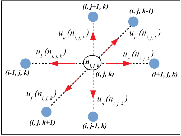
We consider a periodic ZRP lattice in two dimensions of size (). Each site with, , can be vacant or it can be occupied by one or more particle . A particle from any randomly chosen site can hop to its nearest neighbours (right, left, up and down) with rates , , and respectively as shown in Fig. 1.

ZRP does not have an exact steady state when hop rates in all four directions are different. The model is solvable using (a) DB, when the rates and , where both and are constants or and (b) PWB, when all rates , , and differ by a multiplicative constant i.e., the ratios of the rates are independent of , assuming that the model evolves to a FSS
| (1) |
where, the canonical partition function
| (2) |
is the total number of particles and the density of the system is conserved by the dynamics. The steady state weight is defined as
| (3) |
Is it possible to obtain an exact steady state using other flux cancellation schemes for this asymmetric hopping when the hop rates in all four directions are different, that increases the regime of solvability. We consider a new balance condition namely multibalance (MB).
2.1.1 Multibalance (MB)
We define a generalized balance condition in nonequilibrium systems such that a bunch of fluxes coming to the configuration from a set of configurations are balanced by the sum of out-fluxes from to a set of configurations in the configuration space. Here is the total number of incoming fluxes for the set of configurations and is the total number of outgoing fluxes for the set of configurations as described in Fig. 2.

At steady state, for any system, the fluxes must balance: . We have denoted be the probability of the configuration and it can move to the other configuration with a dynamical rate . For systems that satisfy a MB, these steady state configurations break into many conditions of the form,
| (4) |
Eq. (4) describes that for every configuration , the incoming fluxes from a group of configurations , are balanced by outgoing fluxes to another uniquely identified group of configurations . As a special case of MB condition, for , if , Eq. (4) reduces to Pairwise balance balance condition (PWB) and for the simplest case when , it becomes the well known Detailed balance condition (DB) corresponds to the equilibrium case.
2.1.2 Balance Conditions for ZRP Model in two dimensions:
To solve ZRP in two dimensions (see Fig. 1) when the hop rates in all four directions are different, we employ MB condition.
-
1.
A PWB condition, where, the flux, generated, by a particle hopping from site of a configuration to its up nearest neighbour (i.e. site ), can be balanced with the flux due to hopping of a particle from site of another configuration to site . At steady state, PWB condition is satisfied similarly as ZRP model [7], if
(5) -
2.
A MB condition, where, for a configuration , the fluxes generated by a particle hopping to its right and left nearest neighbours from site , can be balanced with the flux obtained by hopping of a particle from site of another configuration to its down nearest neighbour (i.e. site ). The flux balance scheme in Eq. (4) gives the following equation
(6)
Using MB condition one can show that an exact steady state solution is possible and FSS as in Eq. (1) can be obtained only when the hop rates satisfy
| (7) |
As an example, for this particle hopping ZRP model in two dimensions let us define the following rate functions
| (8) | |||||
| (9) |
where the model parameters and is the potential-bias that is taken to be positive. Using the rates in Eqs. (8) and (9) we can obtain the steady state weight following Eq. (3)
| (10) |
2.1.3 Negative differential mobility in two dimensional ZRP
In this section we would like to discuss ZRP in two dimensions with specific choices of rates in Eqs. (8) and (9) give rise to negative differential response [26] of the particles. Following the local detailed balance condition, we can define the driving fields or bias in terms of the asymmetric rate functions as acting on bonds with local configurations for the dynamics
| (11) |
For the set of specific rate functions in Eqs. (8) and (9) we can calculate . The value is excluded as in this case becomes negative.
| (12) |
increases linearly in the positive direction with the increase of the bias parameter for all and . We can express the grand canonical partition function following Eq. (2) as with
| (13) |
where the fugacity controls the particle density through the relation . Finally the current is
| (14) |


To understand the behaviour of current in Eq. (14), we did a Monte Carlo simulation for a fixed particle density and . Fig. 3(a) shows the particle current with the bias parameter for and . For small , current increases as the parameter is increased. Beyond a certain value of where reaches to its maximum value, it decreases with and NDM is observed as soon as . It is evident from Fig. 3(a) that the gradient of current , , decreases with and becomes negative for , which is shown in Fig. 3(b). Current obtained in Eq. (14) may or may not exhibit NDM for every and . To explore the possibility of NDM in this system, we have shown the region where NDM occurs in - phase plane in the inset of Fig. 3(b).
2.2 ZRP in three dimensions with asymmetric rates
We consider a periodic ZRP lattice in three dimensions of size () (see Fig. 4). Each site, represented by can be either vacant or it can be occupied by one or more particles denoted by . From a randomly chosen site , a particle can hop to nearest neighbours (up, down, right, left, frnt and back) with rates , , , , and .
The steady state probability can be defined as
| (15) |
When all rates are different, no general solution is available. One can obtain the FSS as in Eq. (1) for this model using MB condition when the hop rates satisfy the condition
| (16) |
and the steady state weight is defined as . As an example, let us define a simple choices of hop rates
| (17) | |||
| (18) | |||
| (19) |
‘


The grand canonical partition function can be expressed as with and is the Polylogarithm function defined by . Using our choices of rates in Eqs. (17) - (19) we can calculate the currents (right - left direction) and (front - back direction) as
| (20) | |||
| (21) |
In Fig. 5(a) and Fig. 5(b) we have plotted the currents and with the parameter for particle density and . As expected currents in both directions increase linearly with the parameter .
3 Asymmetric finite range process (FRP) with nearest neighbours and next nearest neighbours hopping
We consider one dimensional periodic lattice with sites labeled by (see Fig. 6). Each site has a non negative integer variable , representing the number of particles at site (for a vacant site ). A particle from any randomly chosen site ; can hop to its right nearest neighbour with rate and left nearest neighbour with rate and as well as to the next nearest neighbours with rates for right, for left. All these rates depend on the number of particles at all the sites within a range w.r.t the departure site. This finite range process (FRP), with nearest neighbours hopping has been studied earlier [19, 20].

Like the FRP model discussed in [19], we have considered the steady state probability
| (22) |
where, is the canonical partition function defined as
| (23) |
is the total number of particles and is conserved by the dynamics.
3.1 Balance conditions for asymmetric FRP
We will try to get the steady states of this model for the asymmetric rates. Consider the balance conditions as
-
1.
A PWB condition, where the flux generated due to a particle hopping from site of a configuration to site , can be balanced with the flux obtained by a particle hopping from site of another configuration to site .
(24) (25) Following Eq. (22), one can check that PWB condition as in Eq. (25) will be satisfied if the hop rate at site satisfies the condition as like FRP model [19]
(26) where
-
2.
A MB condition, where fluxes generated due to a particle hopping from site of a configuration to the sites and , can be balanced with the flux obtained by a particle hopping from site of another configuration to its left nearest neighbour site . The flux balance scheme in Eq. (4) gives the following equation
(27) (28) (29)
MB condition as in Eq. (29) for this asymmetric FRP model will be satisfied and one can obtain a cluster-factorized form of steady state (CFSS) as in Eq. (22), when and the hop rates satisfy the condition
| (30) | |||
| (31) |
where
3.2 Conditions for PFSS ()
For , we can obtain the steady states in pair-factorized form using MB, if the hop rates satisfy, following Eq. (31),
| (32) | |||||
| (33) |
Let us consider that the weight function can be written as the inner product of two 2-dimensional vectors [19]
| (34) |
In grand canonical ensemble where the fugacity controls the density , the partition sum can be written as with
| (35) |
Now, for a particular choice of the steady state weight , one can construct the transfer matrix to calculate the density of the system and the correlation function by transfer matrix method in pair-factorized steady state [19].
4 Two species Finite Range Process (FRP)
4.1 The Model
The model is defined on an one dimensional periodic lattice with sites labeled by (see Fig. 7). At each site , there are particles of species (coloured red) and particles of species (cloured blue). Total number of particle is and that of particle is . A particle of any species, from any randomly chosen site can hop to its right nearest neighbour with a rate for species and for species . These two rates depend on the number of particles at all the sites which are within a range w.r.t the departure site like the FRP model [19].

Dynamics of this model can be described as for species
| (36) | |||
| (37) |
and the dynamics of species
| (38) | |||
| (39) |
For , this model is identical to two species zero range process [7] with hop rate for particles of species , and for particles of species , an exactly solvable nonequilibrium model that evolves to a FSS
| (40) |
with the steady state weight
| (41) |
4.1.1 Condition for cluster-factorized steady state (CFSS)
We can express the steady state probability in a cluster factorized form as
| (42) | |||||
| (43) |
where is the canonical partition function defined as
| (44) |
and are total number of particles of species and . and are conserved by the dynamics. We can write the Master equation of this two species FRP model to find the steady state condition
| (45) | |||||
| (46) | |||||
| (47) | |||||
| (48) | |||||
| (49) | |||||
| (50) |
Eq. (50) is true when the gain and loss terms due to the dynamics of species cancel independently of the gain and loss terms due to the dynamics of species . We look to achieve this cancellation for each term in the sum separately. With this condition, the cluster-factorized form of steady states (CFSS) as in Eq. (42) for this two species FRP model is indeed possible when the hop rates of species and satisfy the conditions
| (51) | |||
| (52) | |||
| (53) | |||
| (54) |
where in Eq. (52) and in Eq. (54). These two rates are related by a constraint
| (55) | |||
| (56) |
As like ZRP model with several species of particles [7, 27, 28] , it is possible to generalise FRP to any number of species say . Although there are rates, it is expected that the rates must be related by conditions.
4.2 Two species FRP model with directional asymmetry
We can add a directional asymmetry in two species FRP model (see Fig. 8), by adding conditions, from a randomly chosen site , the particle of species , can hop to its right and left nearest neighbours with rates and , it can hop to right and left next nearest neighbours with rates and . Similarly, particle of species , can hop to its right and left nearest neighbours with rates and , to right and left next nearest neighbours with rates and . All these rates depend on the number of particles at all the sites which are within a range w.r.t the departure site Fig. 8.

4.2.1 Balance conditions for two species FRP model with directional asymmetry
For (PFSS), we can express the steady state probability in terms of the steady state weight following Eq. (42)
| (57) |
where, the canonical partition function
| (58) |
Consider the balance conditions to obtain the steady state
-
1.
PWB conditions, where
(a) Flux generated by hopping of a particle of species from site of a configuration to site , can be balanced with the flux obtained by hopping of a particle of same species from site of another configuration to site .
(b) Similarly, flux generated by hopping of a particle of species from site of the configuration to site , can be balanced with the flux obtained by hopping of a particle of same species from site of another configuration to site . For these PWB conditions with similar argument like Eq. (50), we can calculate rates of species and respectively for as(59) (60) (61) (62) -
2.
MB conditions where
(a) Fluxes generated for a particle of species , hopping from site , of configuration , to sites and , can be balanced with the flux obtained by hopping of a particle of species from site of the configuration to site .
(b) Fluxes generated for a particle of species , hopping from site , of configuration , to sites and , can be balanced with the flux obtained by hopping of a particle of species from site of the configuration to site .
One can verify that pair-factorized form of steady state (PFSS) as in Eq. (57) can be obtained following these MB conditions when the rates , and other hop rates of species and satisfy
| (63) | |||
| (64) |
| (65) | |||
| (66) |
with the rates and are related by a constraint
| (67) |
4.2.2 Observable in two species FRP for K = 1 (PFSS)
Let us consider that the weight function in Eq. (57) can be written by four 2-dimensional vectors as
| (68) |
In grand canonical ensemble, the partition sum following Eq. (58) becomes where, we now have two fugacities and that fix the particle densities of the species and with the transfer matrices
| (69) |
For an example, we consider the 2-dimensional representations as
| (70) | |||
| (71) |
such that the steady state weight becomes
| (72) |
In this case, one can calculate the desired hop rates of both species and species for which the PFSS with the weight function in Eq. (72) is realized. The Transfer matrix following Eq. (69) becomes
| (73) |
and the transfer matrix is just the transpose of the matrix
| (74) |
The eigenvalues of and are and where
| (75) |
The partition function in the thermodynamic limit becomes , as and are the function of and only, we can write the density fugacity relation of species as and for species .

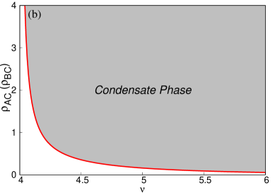
The critical density of species be , and critical density of species , . It turns out that for both species and , for , the critical densities and diverge. For , as and give finite value as shown in Fig. 9 (a), we can say that we have a condensate when densities exceed the critical value for both species. Thus the model exhibits a phase transition between a fluid phase and a condensed phase where the excess particles condense onto a single site. The phase diagram of the condensation transition in - plane is shown in Fig. 9 (b). The critical line separates the condensate phase from the fluid phase.
5 Asymmetric hopping on a triangular lattice
We consider a periodic triangular lattice with sites labeled by (see Fig. 10). Each site has a non negative integer variable , representing the number of particles at site ( if the site is vacant). A particle from any randomly chosen site , can hop to sites and with rates and respectively and can hop to the sites and with rates and . Each of these rates depend on the number of particles of sites . To obtain the steady state of this model for this asymmetric rate, we can consider the steady state probability as

| (76) |
is the total number of particles and is conserved by the dynamics. We will try to obtain the steady state using the MB condition.
5.1 Balance conditions for triangular lattice
-
1.
A PWB condition where flux generated due to a particle hopping from site of the configuration , to site is balanced with the flux obtained by a particle hopping from site of another configuration to site . The flux balance scheme described in Eq. (4) gives the following condition
(77) (78) we can verify that the form of the steady state in pair factorized form as in Eq. (76), is indeed possible when the hop rate at site satisfies the following condition
(79) (80) -
2.
A MB condition where fluxes generated due to the particle hopping from site of the configuration to sites and are balanced by the flux obtained by hopping of a particle from site of another configuration to site . The flux cancellation scheme in Eq. (4) gives the condition
(81) (82) (83)
One can verify that for this model pair-factorized form of steady state (PFSS) as in Eq. (76) is indeed possible using MB and Eq. (83) is satisfied when and the hop rates satisfy the conditions
| (84) | |||
| (85) | |||
| (86) | |||
| (87) |
5.2 Calculation of observable in PFSS
We can express the steady state probability following Eq. (76) as
| (88) |
with and the canonical partition function as
| (89) |
We can rewrite the expression of hop rate in terms of the weight function following Eqs. (80), (88)
| (90) | |||||
| (91) |
and the hop rates and can be chosen accordingly that they satisfy Eq. (87). Let us consider that the weight function can be written by three 2-dimensional representation of matrices [29]
| (92) |
In grand canonical ensemble following Eq. (92), the partition sum can be written as , where is the fugacity and have a relation with the density of the system as and the transfer matrix be
| (93) |
Here, be the identity matrix of the same dimension and we used the fact that direct product of any two vectors and can be written as . Now, with a simple choice of the hop rates, the weight function can be calculated and using transfer matrix following Eq. (93), one can in principle calculate the expectation value of any desired observable [19, 29].
6 Summary
The steady states of non-equilibrium systems are very much dependent on the complexity of the dynamics and it is difficult to track down a systematic procedure to obtain the steady state measure of a system with a given dynamics. In this regard, starting from the Master equation that governs the time evolution of a many particle system in the configuration space, several flux cancellation schemes have been in use for obtaining the exact steady state weight. These schemes include matrix product ansatz (MPA) [14], h-balance scheme [20] and pairwise balance condition (PWB). In this article we introduced a new kind of balance condition, namely multibalance (MB), where the sum of incoming fluxes from a set of configurations to any configuration is balanced by the sum of outgoing fluxes to set of configurations chosen suitably.
We have applied MB condition to a class of nonequilibrium lattice models on a ring where particles hop to its nearest neighbours and for some cases next to nearest neighbours, with a rate that depends on the occupation of all the neighbouring sites within a range. We have solved exactly the asymmetric ZRP in two and three dimensions and discussed that a factorized steady state (FSS) can be obtained when hop rates satisfy a specific condition. More over, the asymmetric ZRP in two dimensions exhibits the phenomena negative differential mobility (NDM) [26]. We have discussed the steady states obtained by MB for asymmetric finite range process (FRP) with nearest neighbours and as well as next nearest neighbours hopping. It gives us a steady state in cluster-factorized form (CFSS) which helps us in calculating the steady state average of the observable using Transfer Matrix method introduced earlier [19].
We have also discussed the two species FRP with directional asymmetry in hop rates and shown that this model too has a CFSS. The model with reduces to the two species zero range process (ZRP) [7] having a FSS. This two species FRP having directional asymmetry, with nearest neighbours and next nearest neighbours hopping, can be solved using the MB condition. The steady state can be obtained for certain conditions on hop rates and one can calculate the steady state observable here. At the last part of our article, we have discussed how this balance condition could be applied for other kind of driven interacting many-particle systems. We have another interesting example, the periodic triangular lattice models (that we introduced here), where a particle from a randomly chosen site can hop to one of its four neighbours with asymmetric rates. MB can be employed to solve this model exactly and obtain a pair factorized steady state (PFSS) under certain conditions on the hop rates.
We should mention that, we have only tried to formulate a new kind of balance condition to obtain the NESS. We emphasized here mainly about the application of this balance condition for different kinds of nonequilibrium models and found the conditions of being steady states. One can easily find out the observable such as density, correlation functions and others at steady state. More importantly, this method could help in finding the exact steady state structure in models even when the interactions extend beyond two sites.
In summary, we introduced a new kind of flux balance condition, namely MB to obtain steady state weights of nonequilibrium systems and demonstrate its utility in many different kinds of non-equilibrium dynamics, including those where the interactions extend beyond two sites. We believe that the MB technique will be very helpful in finding steady state of many other nonequilibrium systems.
References
References
- [1] Schmittmann, B. and Zia, R. K. P., Statistical Mechanics of Driven Diffusive Systems ed. Domb, C. and Lebowitz, J. L., 1995 Academic Press, New York.
- [2] Nonequilibrium Statistical Mechanics In One Dimension, ed. Privman, V., 1997 Cambridge University Press.
- [3] Tolman, R. C. (1938), The Principles of Statistical Mechanics, Oxford University Press, London, UK.
- [4] Boltzmann, L., (1964), Lectures on gas theory, Berkeley, CA, USA: U. of California Press.
- [5] Spitzer, F., Adv. Math. 5, 246 (1970).
- [6] Evans, M.R., Braz. J. Phys. 1, 42 (2000).
- [7] Evans, M.R., and Hanney, T., J. Phys. A: Math. Gen. 38, R195 (2005).
- [8] Kafri, Y., Levine, E., Mukamel, D., Schütz, G.M., and Török, J., Phys. Rev. Lett. 89, 035702 (2002).
- [9] Angel, A.G., Evans, M.R., Levine, E., and Mukamel, D., Phys. Rev. E 72, 046132 (2005).
- [10] Mohanty, P.K., and Jalan, S., Phys. Rev. E 77, 045102(R) (2008).
- [11] Gupta, S., Barma, M., Basu, U., and Mohanty, P.K., Phys. Rev. E 84, 041102 (2011).
- [12] Daga, B., and Mohanty, P.K., J. Stat. Mech. P04004 (2015).
- [13] Schütz, G.M., Ramaswamy, R., Barma, M., J. Phys. A: Math. Gen. 29, 837 (1996).
- [14] Derrida, B., Evans, M.R., Hakim, V., and Pasquier, V., J. Phys. A: Math. Gen. 26, 1493 (1993).
- [15] Blythe, R.A., and Evans, M.R., J. Phys. A: Math. Gen. 40, R333 (2007).
- [16] Evans, M.R., Europhys. Lett. 36, 13. (1996)
- [17] Basu, U., and Mohanty, P.K., Physical Review E 82, 041117,(2010)
- [18] Hinrichsen, H., Sandow, S., and Peschel, I., J. Phys. A: Math. Gen. 29, 2643 (1996).
- [19] Chatterjee, A., Pradhan, P., and Mohanty, P.K., Phys. Rev. E 92, 032103 (2015).
- [20] Chatterjee, A.K., Mohanty, P.K., J. Stat. Mech., 093201, (2017).
- [21] Evans, M.R., Majumdar, S.N., and Zia, R.K.P., J. Phys. A: Math. Gen. 37, L275, (2004).
- [22] Evans, M.R., and Waclaw, B., J. Phys. A: Math. Theor. 47 (2014) 095001.
- [23] Evans, M.R., Hanney, T., and Majumdar, S.N., Phys. Rev. Lett. 97, 010602 (2006).
- [24] Levine, E., Mukamel, D., and Schütz, G.M., J Stat Phys 120, 759 (2005).
- [25] Bertin, E., Vanicat, M., J. Phys. A: Math. Theor. 51, 245001, (2018).
- [26] Chatterjee, A.K., Basu, U., and Mohanty, P.K., Phys. Rev. E 97, (2018).
- [27] Hanney, T., and Evans, M.R., Phys. Rev. E 69, 016107
- [28] Grosskinsky, S., Spohn, H., Bull. Braz. Math. Soc. 34(3), 489-507 (2003)
- [29] Chatterjee, A.K., Mohanty, P.K., J. Phys. A: Math. Theor. 50, 495001, (2017).