Multi-task manifold learning for small sample size datasets

Multi-task learning is a paradigm of machine learning that aims to improve performance by learning similar tasks simultaneously [7, 8]. Many studies have been conducted on multi-task learning, particularly in supervised learning settings. By contrast, few studies have been conducted on multi-task unsupervised learning. Some studies on multi-task clustering have been reported [9, 10, 11, 12].

To date, few studies have been conducted on dimensionality reduction, subspace methods, and manifold learning. To the best of our knowledge, a study on multi-task principal component analysis (PCA) is the only research that is expressly aimed at the multi-task learning of subspace methods [13]. In multi-task PCA, the given datasets are modeled by linear subspaces, which are regularized so that they are closed to each other on the Grassmannian manifold.

Regarding nonlinear subspace methods, to the best of our knowledge, the most closely related work is the higher-order self-organizing map (SOM², which is also called the ‘SOM of SOMs’) [14, 15]. Although SOM² is designed for multi-level modeling rather than multi-task learning, the function of SOM² can also be regarded as multi-task learning. SOM² is described in detail below.

Multi-level modeling (or hierarchical modeling) aims to obtain higher models of tasks in addition to modeling each task [16]. Although multi-level modeling does not aim to improve the performance of individual tasks, the research areas of multi-level modeling and multi-task learning overlap. In fact, multi-level modeling is sometimes adopted as an approach for multi-task learning [17, 18, 19].

As in the case of multi-task learning, most studies conducted on multi-level modeling have considered supervised learning, particularly linear models. Among the multi-level unsupervised modeling approaches, SOM² aims to model a set of self-organizing maps (SOMs) using a higher-order SOM (higher-SOM) [14, 15]. In SOM², the lower-order SOMs (lower-SOMs) model each task using a nonlinear manifold, whereas the higher-SOM models those manifolds by another nonlinear manifold in function space. As a result, the entire dataset is represented by a product manifold, that is, a fiber bundle. Thus, the manifolds represented by the lower-SOMs are the fibers, whereas the higher-SOM represents the base space of the fiber bundle. Additionally, the relations between tasks are visualized in the low-dimensional space of the tasks, in which similar tasks are arranged nearer to each other and different tasks are arranged further from each other.

The learning algorithm of SOM² is not a simple cascade of SOMs. The higher and lower-SOMs learn in parallel and affect each other. Thus, whereas the higher-SOM learns the set of lower models, the lower-SOMs are regularized by the higher-SOM so that similar tasks are represented by similar manifolds. Thus, SOM² has many aspects of multi-task learning. In fact, SOM² has been applied to several areas of multi-task learning, such as unsupervised modeling of face images of various people [20], nonlinear dynamical systems with latent state variables [21, 22], shapes of various objects [23, 24], and people of various groups [25, 26]. In this sense, SOM² is one of the earliest works on multi-task unsupervised learning for nonlinear subspace methods.

Although SOM² works like multi-task learning, it is still difficult for it to estimate manifolds when the sample size is small. Additionally, SOM² has several limitations that originate from SOM, such as poor manifold representation caused by the discrete grid nodes. In this study, we try to overcome these limitations of SOM² by replacing SOM with KSMM. Then we extend it for multi-task learning so that it estimates the manifold shape more accurately, even for a small sample size.

Recently, the concept of meta-learning has been gaining importance [6]. Meta-learning aims to solve unseen future tasks efficiently through learning multiple existing tasks. This is in contrast to multi-task learning, which aims to improve the learning performance of existing tasks. Because MT-KSMM aims to obtain a general model that can represent future tasks in addition to existing tasks, our aim covers both multi-task learning and meta-learning. Similar to the cases of multi-task learning and multi-level learning, meta-learning of unsupervised learning has rarely been performed. Particularly, to the best of our knowledge, meta-learning in an unsupervised manner of unsupervised learning has not been reported, except SOM². In this sense, SOM² is a method in a unique position. In this study, we aim to develop a novel method for multi-task, multi-level, and meta-learning of manifold models based on SOM².

Nonlinear methods for dimensionality reduction are roughly categorized into two groups. The first group is methods that project data points from high-dimensional space to low-dimensional space. Most dimensionality reduction methods, including many manifold learning approaches, are classified in this group. By contrast, the second group explicitly estimates the mapping from low-dimensional latent space to the manifold in high-dimensional visible space [27]. Thus a nonlinear embedding is estimated by this group. Because new samples on the manifold can be generated by using the estimated embedding, we refer to the second group as generative manifold modeling in this study. An advantage of generative manifold model is that it does not suffer from the pre-image problem and the out-of-sample extension problem [28]. Thus, by generating new samples between the given data points, generative manifold model completes the manifold shape entirely. Additionally, because the embedding is explicitly estimated, generative manifold model allows the direct measurement of the distance between two manifolds in function space. These are the reasons that we chose the generative manifold model approach.

The representative methods of generative manifold modeling are generative topographic mapping (GTM) [29], the Gaussian process latent variable model (GPLVM) [30, 27], and unsupervised kernel regression (UKR) [31], which originate from the SOM [32]. To estimate the embedding and the latent variables, GPLVM and GTM employ the Bayesian approach that use a Gaussian process, whereas UKR and SOM employ the non-Bayesian approach that use a kernel smoother. Additionally, GPLVM and UKR represent the manifold in a non-parametric manner, whereas GTM and SOM represent it in parametric manner. In this study, we use a parametric kernel smoothing approach like the original SOM, for ease of information transfer between tasks.

In nonlinear subspace methods, there is always arbitrariness in the determination of the coordinate system of the latent space. For example, any orthogonal transformation of the latent space yields an equivalent result. Additionally, any nonlinear distortion along the manifold is also allowed.

In single-task learning, such arbitrariness is not a problem, but it causes serious problems in multi-task learning. Because the coordinate system of the latent space is determined differently for each task, the learning results become incompatible between tasks. Therefore, it prevents knowledge transfer between tasks.

To solve this problem, we need to know the correspondences between two different manifolds, or we need to regularize them so that they share the same coordinate system. This is known as the manifold alignment problem, which is challenging to solve under the unsupervised condition [33]. This is one reason why the multi-task subspace method is difficult. In the case of multi-task PCA, they escaped this problem by mapping them to a Grassmannian manifold [13]; however, this approach is only possible for the linear subspace case. Therefore, manifold alignment is an unavoidable problem, which is challenged in this study.

First, we describe the problem formulation for the single-task case (Figure 1 (a)). Let ${\cal V}=\mathbb{R}^{{D_{\cal V}}}$ and ${\cal L}\subseteq\mathbb{R}^{{D_{\cal L}}}$ be high-dimensional visible space and low-dimensional latent space, respectively, and let $X=\bigl{\{}\mathbf{x}_{n}\bigr{\}}_{n=1}^{N}$ be the observed sample set, where $\mathbf{x}_{n}\in{\cal V}$. In the case of a face image dataset, $X$ is the set of face images of a single person with various expressions or poses, and $\mathbf{z}_{n}\in\EuScript{L}$ is the sample latent variable corresponding to $\mathbf{x}_{n}$, which represents the intrinsic property of the image, such as the expression or pose. The main purpose of manifold learning is to map $X$ to ${\cal L}$ by assuming that sample set $X$ is modeled by a manifold ${\cal X}\subseteq{\cal V}$, which is homeomorphic to ${\cal L}$. Thus, a homeomorphism $\pi\colon{\cal X}\xrightarrow{\sim}{\cal L}$ can be defined, by which $\mathbf{x}\in{\cal X}$ is projected to $\mathbf{z}=\pi(\mathbf{x})$. Note that actual samples are not distributed in ${\cal X}$ exactly because of observation noise. Thus, the observed sample $\mathbf{x}_{n}$ is represented as $\mathbf{x}_{n}=\pi^{-1}(\mathbf{z}_{n})+{\boldsymbol{\varepsilon}}_{n}$, where ${\boldsymbol{\varepsilon}}_{n}\sim{\cal N}(\mathbf{0},\beta^{-1}\mathbf{I}_{{D_{\cal V}}})$ is observation noise. Generative manifold modeling not only aims to estimate the sample latent variables $Z=\left\{\mathbf{z}_{n}\right\}_{n=1}^{N}$, but also to estimate the embedding $f\coloneqq\pi^{-1}$ explicitly. Thus, the probabilistic generative model is estimated as $q(\mathbf{x},\mathbf{z}\mid f)={\cal N}(\mathbf{x}\mid f(\mathbf{z}),\beta^{-1}\mathbf{I}_{D_{\cal V}})\,p(\mathbf{z})$. Because $f$ is expected to be a smooth continuous mapping, we assume that $f$ is a member of a reproducing kernel Hilbert space (RKHS) ${\cal H}=\{f\mid f\colon{\cal L}\to{\cal V}\}$.

Now we formulate the problem in which we have $I$ tasks. Thus, we have $I$ sample sets $\bigl{\{}X_{1},\dots,X_{I}\bigr{\}}$, where $X_{i}=\bigl{\{}\mathbf{x}_{ij}\bigr{\}}_{j=1}^{J_{i}}$. For example, in the case of face image datasets, we have $I$ image sets of $I$ people, with $J_{i}$ expressions or poses for each person. We denote the entire sample set by $X=\bigcup_{i}X_{i}=\bigl{\{}\mathbf{x}_{n}\bigr{\}}_{n=1}^{N}$, where $N=\sum_{i}J_{i}$. We also denote the entire sample set by matrix $\mathbf{X}=\bigl{(}\mathbf{x}^{\mathsf{T}}_{n}\bigr{)}\in\mathbb{R}^{N\times D_{\cal V}}$. In the same manner, $Z_{i}=\left\{\mathbf{z}_{ij}\right\}_{j=1}^{J_{i}}$ is the latent variable set of task $i$, which corresponds to $X_{i}$, whereas the entire latent variable set is represented as $Z=\left\{\mathbf{z}_{n}\right\}_{n=1}^{N}$. Additionally, let $i_{n}$ be the task index of sample $n$, and let ${\cal N}_{i}$ be the index set of samples that belong to task $i$. To simplify the explanation, we consider the case in which each dataset has the same number of samples (sample per task: S/T), that is, $J_{i}\equiv J$.

Similar to the single-task case, we assume that $\{X_{i}\}$ is modeled by manifolds $\{{\cal X}_{i}\}$, which are all homeomorphic to the common latent space ${\cal L}\subseteq\mathbb{R}^{{D_{\cal L}}}$. Thus, we can define a smooth embedding $f_{i}\colon{\cal L}\to{\cal X}_{i}\subseteq{\cal V}$ for each task, where $f_{i}\coloneqq\pi_{i}^{-1}$ (Figure 1 (b)). By considering the observation noise, we represent the probability distribution of task $i$ by $q_{i}(\mathbf{x},\mathbf{z}\mid f_{i})={\cal N}(\mathbf{x}\mid f_{i}(\mathbf{z}),\beta^{-1}\mathbf{I}_{D_{\cal V}})\,p(\mathbf{z})$. In this study, the individual embedding $f_{i}$ is referred to as the task model.

To apply multi-task learning, the given tasks need to have some similarities or common properties. We make the following two assumptions on the similarities of tasks. First, the sample latent variable $\mathbf{z}$ represents the intrinsic property of the sample, which is independent of the task. Thus, if $\mathbf{x}_{ij}$ and $\mathbf{x}_{i^{\prime}j^{\prime}}$ are mapped to the same $\mathbf{z}$, they are regarded as having the same intrinsic property, even if $\mathbf{x}_{ij}\neq\mathbf{x}_{i^{\prime}j^{\prime}}$. For example, if both $\mathbf{x}_{ij}$ and $\mathbf{x}_{i^{\prime}j^{\prime}}$ are face images of different people with the same expression (e.g., smiling), they should be mapped to the similar $\mathbf{z}$, even if the images look different. Using this assumption, the distance between two manifolds ${\cal X}_{i}$ and ${\cal X}_{i^{\prime}}$ can be defined using the norm $\left\|f_{i}-f_{i^{\prime}}\right\|_{\cal H}$ as

where $dP(\mathbf{z})$ is the measure of $\mathbf{z}$, which is common to all tasks. In this study, we define the measure as $dP(\mathbf{z})=p(\mathbf{z})\,d\mathbf{z}$, where $p(\mathbf{z})$ is the prior of $\mathbf{z}$.

Second, we assume that the set of task models $F=\{f_{i}\}_{i=1}^{I}$ is also distributed in a nonlinear manifold ${\cal Y}$ embedded into RKHS ${\cal H}$ (Figure 1 (c)). Thus, ${\cal Y}$ is defined by a nonlinear smooth embedding $g\colon{\cal T}\to{\cal Y}\subseteq{\cal H}$, where ${\cal T}\subseteq\mathbb{R}^{{D_{\cal T}}}$ is the low-dimensional latent space for tasks. Under this assumption, all tasks are assigned to the task latent variables $U=\{\mathbf{u}_{i}\}_{i=1}^{I}$, $\mathbf{u}_{i}\in{\cal T}$ so that $f_{i}=g(\mathbf{u}_{i})$. It also means that if $i$ and $i^{\prime}$ are similar, then $\mathbf{u}_{i}\sim\mathbf{u}_{i^{\prime}}$ and ${\cal X}_{i}\sim{\cal X}_{i^{\prime}}$. As a result, the entire model distribution is represented as

where $G\colon{\cal L}\times{\cal T}\to{\cal E}\subseteq{\cal V}$ is defined as $G(\cdot,\mathbf{u})=g(\mathbf{u})$, and $\EuScript{E}$ is the embedded product manifold of ${\cal L}\times{\cal T}$ into ${\cal V}$ (Figure 1 (d)). In this study, $G$ is referred to as the general model. Using the general model, each task model is expected to be $f_{i}(\mathbf{z})=G(\mathbf{z},\mathbf{u}_{i})$.

We can describe this problem formulation using the terms of the fiber bundle. Suppose that ${\cal E}\subseteq{\cal V}$ is the total space of the fiber bundle, where ${\cal E}\coloneqq G\left({\cal L},{\cal T}\right)$. Then we can define a projection $\eta\colon{\cal E}\rightarrow{\cal T}$ so that $\eta({\cal X}_{i})\equiv\mathbf{u}_{i}$, where ${\cal T}$ is now referred to as the base space. Thus, the samples that belong to the same task are all projected to the same $\mathbf{u}$. Under this scenario, $({\cal E},{\cal T},\eta)$ becomes a fiber bundle, and each task manifold ${\cal X}_{i}$ is regarded as a fiber. Additionally, we can define another projection $\pi\colon{\cal E}\rightarrow{\cal L}$, which satisfies $\pi(\mathbf{x}_{ij})\equiv\pi_{i}(\mathbf{x}_{ij})$. Such a formulation using the fiber bundle has been proposed in some studies [14, 34].

Under this scenario, our aim is to determine the general model $G$ in addition to the task model set $F=\bigl{\{}f_{i}\bigr{\}}_{i=1}^{I}$, and to estimate the latent variables of samples $Z=\left\{\mathbf{z}_{n}\right\}_{n=1}^{N}$ and tasks $U=\left\{\mathbf{u}_{i}\right\}_{i=1}^{I}$. Considering compatibility with SOM, we assume that the latent spaces are square spaces ${\cal L}=[-1,+1]^{D_{\cal L}}$ and ${\cal T}=[-1,+1]^{D_{\cal T}}$, and the priors $p(\mathbf{z})$ and $p(\mathbf{u})$ are the uniform distribution on ${\cal L}$ and ${\cal T}$¹¹1Rigorously speaking, we need to consider the border effect in the case of compact latent space, such as $[-1,+1]^{D}$. In this study, we ignore such a border effect for ease of implementation. Such an approximation is common in SOM and its variations.. The difficulty of learning depends on S/T (i.e., $J$) and the number of tasks $I$. Particularly, we are interested in the case in which S/T is too small to capture the manifold shape, whereas we have a sufficient number of tasks for multi-task learning.

We chose KSMM as a generative manifold modeling method, which estimates the embedding using a kernel smoother. Thus, our aim is to develop the multi-task KSMM, that is, MT-KSMM. KSMM is a theoretical generalization of SOM, which has been proposed in many studies [35, 36, 37, 38, 39]. The main difference between SOM and KSMM is that the former discretizes the latent space ${\cal L}$ to regular grid nodes, whereas the latter treats it as continuous space. According to previous studies, the cost function of KSMM is given by

where $h_{\cal L}(\mathbf{z}\mid\mathbf{z}^{\prime})$ is the non-negative smoothing kernel defined on ${\cal L}$, which is typically $h_{\cal L}(\mathbf{z}\mid\mathbf{z}^{\prime})={\cal N}\bigl{(}\mathbf{z}\,|\,\mathbf{z}^{\prime},\lambda_{\cal L}^{2}\mathbf{I}\bigr{)}$ [38]. If we regard $h_{\cal L}(\mathbf{z}\mid\mathbf{z}^{\prime})$ as the probability density that represents the uncertainty of $\mathbf{z}_{n}$, the cost function (3) equals the cross-entropy between the data distribution $p(\mathbf{x},\mathbf{z})$ and the model distribution $q(\mathbf{x},\mathbf{z})$ (ignoring the constant), which are given by

Thus, $E[Z,f\mid X]\stackrel{{\scriptstyle c}}{{=}}H[p(\mathbf{x},\mathbf{z}\mid X,Z),q(\mathbf{x},\mathbf{z}\mid f)]$, where ‘$\stackrel{{\scriptstyle c}}{{=}}$’ means that both hands are equal except the constant, and $H[\cdot,\cdot]$ denotes the cross-entropy.

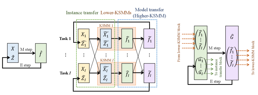
The KSMM algorithm is the expectation maximization (EM) algorithm in the broad sense [38, 39], in which the E and M steps are iterated alternately until the cost function (3) converges (Figure 2 (a)). In the E step, the cost function (3) is optimized with respect to $Z$, whereas $f$ is fixed as follows:

where $\hat{\mathbf{z}}_{n}$ and $\hat{f}$ represent the estimators of $\mathbf{z}_{n}$ and $f$, respectively²²2In this study, the (tentative) estimators are denoted by hat $\hat{\ }$ when we need to indicate expressly. We also denote the information transfer result by tilde $\tilde{\ }$.. The latent variable estimation obtained by (7) is used in the original SOM [32] and some similar methods [31]. Note that we can rewrite (7) as

which means the maximum log-likelihood estimator. We optimize (7) using SOM-like grid search to avoid local minima for early loops of iterations, and then they are updated by the gradient method in the later loops.

By contrast, in the M step, (3) is optimized with respect to $f$, whereas $Z$ is fixed, as follows:

The solution of (8) is given by the kernel smoothing of samples as

These E and M steps are executed repeatedly until the cost function (3) converges. In the proposed method, embedding $f$ is represented parametrically using orthonormal bases. The details are provided in Section 4.5.

There are several reasons why we chose kernel smoothing-based manifold modeling rather than Gaussian process-based modeling. First, because KSMM is a generalization of SOM, it is easy to extend SOM² to MT-KSMM naturally. Second, because the information transfers are made by the non-negative mixture of datasets or models, a kernel smoother can be used consistently through the method. Third, because the kernel smoother acts as an elastic net that connects the data points [40, 41], the kernel smoothing of task models is expected to solve the unsupervised manifold alignment problem by minimizing the distance between manifolds. Finally, as far as we examined, kernel smoothing-based manifold modeling is more stable and less sensitive to sample variations than the Gaussian process. This property seems to be desirable for multi-task learning, particularly when the sample size is small.

For multi-task learning, the information about each task needs to be transferred to other tasks. Generally, there are three major approaches: feature-based, parameter-based, and instance-based [8]. To summarize, the feature-based approach transfers or shares the intrinsic representation between tasks, the parameter-based approach transfers the model parameters between tasks, and the instance-based approach shares the datasets among the tasks. In the proposed method, we use two information transfer styles: model transfer, which corresponds to the parameter-based approach, and instance transfer, which corresponds to the instance-based approach. Although we do not use the feature-based approach explicitly in the proposed method, we can regard the latent space ${\cal L}$, which is common to all tasks, as the intrinsic representation space shared among the tasks. Therefore, the proposed method is related to all information transfer styles of multi-task learning.

In instance transfer, samples of a task are transferred to other tasks, and form a weighted mixture of samples. Thus, if task $i^{\prime}$ is a neighbor of task $i$ in the task latent space ${\cal T}$, the sample set $X_{i^{\prime}}$ is merged with the target set $X_{i}$ as an auxiliary sample set with a larger weight. By contrast, if task $i^{\prime\prime}$ is far from task $i$ in ${\cal T}$, then $X_{i^{\prime\prime}}$ is merged with $X_{i}$ with a small (or zero) weight. We denote the weight of sample $n$ in source task $i_{n}$ with respect to the target task $i$ by $\rho_{in}$ ($0\leq\rho_{in}\leq 1$). Typically $\rho_{in}$ is defined as

where $\lambda_{\rho}$ determines the neighborhood size for data mixing, and $\hat{\mathbf{u}}_{i}$ is the estimator of the task latent variable $\mathbf{u}_{i}$. Then we have the merged dataset $\tilde{X}_{i}=\{(\mathbf{x}_{n},\rho_{in})\}$, where $(\mathbf{x}_{n},\rho_{in})\in\tilde{X}_{i}$ indicates that $\mathbf{x}_{n}$ is a member of $\tilde{X}_{i}$ with weight $\rho_{in}$. Similarly, the latent variable set $Z_{i}$ is also merged with the same weight as $\tilde{Z}_{i}=\left\{(\hat{\mathbf{z}}_{n},\rho_{in})\right\}$. The data distribution corresponding to the merged dataset $(\tilde{X}_{i},\tilde{Z}_{i})$ becomes

where $\tilde{J}_{i}=\sum_{n}\rho_{in}$. Eq. (11) means that the data distributions $P=\{p_{i}\}$ are smoothed by kernel $\rho(\mathbf{u},\mathbf{u}^{\prime})$ before the task models are estimated. By creating a weighted mixture of samples, we can avoid the small sample set problem.

By contrast, in model transfer, each task model $f_{i}$ is modified so that it becomes similar to the models of the neighboring tasks, as follows:

where $h_{\cal T}(\mathbf{u}\mid\mathbf{u}^{\prime})={\cal N}(\mathbf{u}\mid\mathbf{u}^{\prime},\lambda^{2}_{\cal T}\mathbf{I})$. Eq. (12) means the kernel smoothing of the task models $F=\{f_{i}\}$. Thus, the model distribution becomes

Note that (12) and (13) are integrated as

Therefore, the log of model distributions $Q=\{q_{i}\}$ is smoothed by kernel $h_{\cal T}(\mathbf{u}\mid\mathbf{u}^{\prime})$ after the task models are estimated.

When we have $I$ datasets (i.e., $I$ tasks), we need to execute $I$ KSMMs in parallel. To execute the multi-task learning of KSMMs, the proposed method MT-KSMM introduces two key ideas. The first idea is to use both instance transfer and model transfer, and the second idea is to introduce the higher-KSMM, which integrates the $I$ manifold models estimated by the KSMMs for tasks (i.e., the lower-KSMMs).

As described in 4.1, KSMM estimates $\hat{f}$ from $X$ and $\hat{Z}$ in the M step, whereas $\hat{Z}$ is estimated from $X$ and $\hat{f}$ in the E step. The first key idea is to use the merged dataset $(\tilde{X}_{i},\tilde{Z}_{i})$ that is obtained by instance transfer instead of using the original dataset $(X_{i},\hat{Z}_{i})$. Thus, $\hat{f}_{i}$ is estimated from $\tilde{X}_{i}$ and $\tilde{Z}_{i}$. Similarly, to estimate the latent variables $\hat{Z}_{i}$, the proposed method uses the embedding $\tilde{f}_{i}$ that is obtained using model transfer instead of using $\hat{f}_{i}$ directly (Figure 2 (b)).

To execute instance transfer and model transfer, we need to determine the similarities between tasks. For this purpose, the proposed method introduces the higher-KSMM (Figure 2 (c)). Thus, the higher-KSMM estimates the latent variables of tasks $\hat{U}=\left\{\hat{\mathbf{u}}_{i}\right\}_{i=1}^{I}$, by which the similarities between tasks are determined. Another important role of the higher-KSMM is to make the model transfer by estimating the general model $\hat{G}$ from the task models $\hat{F}=\{\hat{f}_{i}\}_{i=1}^{I}$.

After introducing these two key ideas, the entire architecture of MT-KSMM consists of three blocks: the instance transfer block, lower-KSMM block, and higher-KSMM block (i.e., the model transfer block) (Figure 2 (b)). The aim of the lower-KSMM is to estimate the task models $f_{i}$ for each task $i$ from the merged dataset $(\tilde{X}_{i},\tilde{Z}_{i})$. Without considering information transfer, the cost function of the lower KSMM for task $i$ is given by

However, the minimization of the cost function is affected by the information transfer at every iteration of the EM algorithm. Thus, before executing the M step, $(X_{i},\hat{Z}_{i})$ are merged by the instance transfer as $(\tilde{X}_{i},\tilde{Z}_{i})$, whereas before executing the E step, $\hat{f}_{i}$ is replaced by $\tilde{f}_{i}$ as a result of model transfer.

By contrast, the aim of the higher-KSMM is to estimate the general model $G$ by regarding the task models $\hat{F}=\{\hat{f}_{i}\}_{i=1}^{I}$ as the dataset. Thus, the cost function (without considering the influence of other blocks) is given by

This cost function equals the cross-entropy between $p(\mathbf{x},\mathbf{z},\mathbf{u}\mid\hat{F},U)$ and $q(\mathbf{x},\mathbf{z},\mathbf{u}\mid G)$ as

where

Note that $p(\mathbf{x},\mathbf{z},\mathbf{u})$ is determined by $\hat{F}=\{\hat{f}_{i}\}$ and $U=\{\mathbf{u}_{i}\}$, regarding $\hat{F}=\{\hat{f}_{i}\}$ as the input data. Therefore, $p(\mathbf{x},\mathbf{z},\mathbf{u})$ is not determined by the observed samples $X$ naively; thus,

The lower and higher-KSMMs do not simply optimize the cost functions (15) and (16) in parallel. The estimated task models $\hat{F}=\{\hat{f}_{i}\}_{i=1}^{I}$ are fed forward to the higher-KSMM from the lower-KSMM as the dataset, whereas the estimated general model $\hat{G}$ is fed back from the higher to the lower as a result of model transfer, so that $\tilde{f}_{i}(\cdot)=\hat{G}(\cdot,\hat{\mathbf{u}}_{i})$. Additionally, the estimated task latent variables $\hat{U}=\{\hat{\mathbf{u}}_{i}\}_{i=1}^{I}$ are also fed back from the higher-KSMM to the instance transfer block, whereby the merged datasets $\{(\tilde{X}_{i},\tilde{Z}_{i})\}_{i=1}^{I}$ are updated. Such a hierarchical optimization process satisfies the concept of meta-learning [6].

The MT-KSMM algorithm is described as follows (also see Algorithm 1).

Step 0:

Initialization

For the first loop, the latent variables $\hat{Z}=\left\{\hat{\mathbf{z}}_{n}\right\}$ and $\hat{U}=\left\{\hat{\mathbf{u}}_{i}\right\}$ are initialized randomly.

Step 1:

Instance transfer

To execute instance transfer, $\rho_{in}$ is calculated using (10). Then we have the merged datasets $\tilde{X}_{i}=\{(\mathbf{x}_{n},\rho_{in})\}$ and $\tilde{Z}_{i}=\{(\mathbf{z}_{n},\rho_{in})\}$ for all $i$. This step can be interpreted as the kernel smoothing of the data distribution set $P=\{p_{i}(\mathbf{x},\mathbf{z})\}$ using (11), and we have $\tilde{P}=\{\tilde{p}_{i}(\mathbf{x},\mathbf{z})\}$ as a result.

Step 2:

M step of the lower-KSMM

Task models $\hat{F}=\{\hat{f}_{i}\}$ are updated so that the cost function of the lower-KSMM is minimized as

$\displaystyle\hat{f}_{i}$

$\displaystyle\coloneqq\operatorname*{\arg\min}_{f_{i}}E_{i}^{\text{lower}}[\tilde{Z}_{i},f_{i}\mid\tilde{X}_{i}],$

for each task $i$. The solution is given by the kernel smoothing of the merged sample set as follows:

$\displaystyle\hat{f}_{i}(\mathbf{z})$

$\displaystyle\coloneqq\frac{\sum_{n}h_{\cal L}(\mathbf{z},\hat{\mathbf{z}}_{n})\rho_{in}\,\mathbf{x}_{n}}{\sum_{n^{\prime}}h_{\cal L}(\mathbf{z},\hat{\mathbf{z}}_{n^{\prime}})\rho_{in}}.$

(17)

Then we have the model distribution set $Q=\{\hat{q}_{i}(\mathbf{x},\mathbf{z})\}$ by (5).

Step 3:

M step of the higher-KSMM

The general model $\hat{G}$ is updated so that the cost function of the higher-KSMM is minimized as

$\displaystyle\hat{G}$

$\displaystyle\coloneqq\operatorname*{\arg\min}_{G}E^{\text{higher}}[\hat{U},G\mid\hat{F}].$

The solution is given by

$\displaystyle\hat{G}(\mathbf{z},\mathbf{u})$

$\displaystyle\coloneqq\frac{\sum_{i}h_{\cal T}(\mathbf{u},\hat{\mathbf{u}}_{i})\,\hat{f}_{i}(\mathbf{z})}{\sum_{i^{\prime}}h_{\cal T}(\mathbf{u},\hat{\mathbf{u}}_{i^{\prime}})}.$

(18)

Then we have the entire model distribution $q(\mathbf{x},\mathbf{z},\mathbf{u}\mid\hat{G})$ using (2). This process is regarded as model transfer.

Step 4:

E step of the higher-KSMM

The task latent variables $\hat{U}=\{\mathbf{u}_{i}\}$ are updated so that the log-likelihood is maximized as

	$\displaystyle\hat{\mathbf{u}}_{i}$	$\displaystyle\coloneqq\operatorname*{\arg\max}_{\mathbf{u}_{i}}\sum_{n\in{\cal N}_{i}}\log q(\mathbf{x}_{n},\hat{\mathbf{z}}_{n},\mathbf{u}_{i}\mid\hat{G})$
		$\displaystyle=\operatorname*{\arg\min}_{\mathbf{u}_{i}}\sum_{n\in{\cal N}_{i}}\left\|\hat{G}(\hat{\mathbf{z}}_{n},\mathbf{u}_{i})-\mathbf{x}_{n}\right\|^{2}.$		(19)

Then we have the task models as

	$\displaystyle\tilde{f}_{i}(\mathbf{z})$	$\displaystyle:=\hat{G}(\mathbf{z},\hat{\mathbf{u}}_{i})$
	$\displaystyle\tilde{q}_{i}(\mathbf{x},\mathbf{z})$	$\displaystyle:=q(\mathbf{x},\mathbf{z}\mid\hat{\mathbf{u}}_{i},\hat{G}),$

which are the results of model transfer using (12) and (13). Then $\tilde{F}=\{\tilde{f}_{i}\}$ is fed back to the lower-KSMM.

Step 5:

E step of the lower-KSMM

Finally, the sample latent variables $\hat{Z}=\{\mathbf{z}_{n}\}$ are updated so that the log-likelihood is maximized as

	$\displaystyle\hat{\mathbf{z}}_{n}$	$\displaystyle\coloneqq\operatorname*{\arg\max}_{\mathbf{z}_{n}}\log\tilde{q}_{i_{n}}(\mathbf{x}_{n},\mathbf{z}_{n})$
		$\displaystyle=\operatorname*{\arg\min}_{\mathbf{z}_{n}}\left\|\tilde{f}_{i_{n}}(\mathbf{z}_{n})-\mathbf{x}_{n}\right\|^{2}.$		(20)

These five steps are iterated until the calculation converges. During the iterations, the length constant of the smoothing kernels $\lambda_{\cal L}$ and $\lambda_{\cal T}$ are gradually reduced just like the ordinary SOM.

To apply the gradient method, we represent embedding $f$ parametrically using orthonormal basis functions defined on the RKHS (e.g., normalized Legendre polynomials), such as

where ${\boldsymbol{\varphi}}=(\varphi_{1},\dots,\varphi_{L})^{\mathsf{T}}$ is the basis set and $\mathbf{V}\in\mathbb{R}^{L\times D_{\EuScript}{X}}$ is the coefficient matrix. In the case of single-task KSMM, the estimator of the coefficient matrix $\hat{\mathbf{V}}$ is determined as

where

and

Thus, (9) is replaced by (21)–(25).

Similarly, in MT-KSMM, the coefficient matrices of the task models are estimated as

where

Thus, (17) is replaced by (26)–(30). Note that $\underline{\mathbf{V}}=(\mathbf{V}_{i})_{i=1}^{I}\in\mathbb{R}^{I\times L\times{D_{\cal V}}}$ becomes a tensor of order 3. For the higher-KSMM, the general model $G$ is represented as

where $\underline{\mathbf{W}}\in\mathbb{R}^{K\times L\times{D_{\cal V}}}$ is the coefficient tensor and $\times_{m}$ represents the tensor–matrix product, where ${\boldsymbol{\psi}}=(\psi_{1},\dots,\psi_{K})^{\mathsf{T}}$ is the basis set for the higher-KSMM. The coefficient tensor $\underline{\mathbf{W}}$ is estimated as

where

Thus, (18) is replaced by (32)–(36). Note that the computational cost of the proposed method with respect to the data size is ${\cal O}(NID_{\cal V})$ for the lower-KSMMs and ${\cal O}(ID_{\cal V})$ for the higher-KSMM. Therefore, the computation cost is proportional to both the data size $N$ and number of tasks $I$.

To demonstrate the performance of the proposed method, we applied the method to three datasets. The first was an artificial dataset generated from two-dimensional (2D) manifolds, and the second and third were face image datasets of multiple subjects with various poses and expressions, respectively.

To examine how the information transfer improved performance, we compared methods that used different transfer styles, and KSMM was used for all methods as the common platform. Thus, (1) MT-KSMM (the proposed method) used both instance transfer and model transfer, (2) KSMM² (the preceding method) used model transfer only, and (3) single-task KSMM did not transfer information between tasks³³3It is not able to examine the case of using instance transfer only because the task latent variable $\hat{U}=\{\hat{\mathbf{u}}_{i}\}$ cannot be estimated without using the higher-KSMM, which also makes the model transfer.. KSMM² is a modification of the preceding method SOM² that replaces the higher and lower-SOMs with KSMMs. Note that this modification improves the performance of SOM² by eliminating the quantization error. Similarly, single-task KSMM can be regarded as a SOM with continuous latent space.

In the experiment, we trained the methods on a set of tasks by changing S/T. After training was complete, we evaluated the performance both qualitatively and quantitatively using the test data. We used two types of test data: test data of existing tasks and test data of new tasks. The former evaluates the generalization performance for new data of existing tasks that have been learned, and the latter evaluates the generalization performance for new unknown tasks.

We assessed the learning performance quantitatively using two approaches: the root mean square error (RMSE) of the reconstructed samples and the mutual information (MI) between the true and estimated sample latent variables. RMSE (smaller is better) evaluates accuracy in the visible space ${\cal V}$ without considering the compatibility of the sample latent variables, whereas MI (larger is better) evaluates accuracy in the latent space ${\cal L}$, and considers how consistent the sample latent variables are between tasks. We evaluated both RMSE and MI for the test data of existing tasks and new tasks. For existing tasks, we used the task latent variable $\hat{\mathbf{u}}_{i}$ that was estimated in the training phase, whereas $\hat{\mathbf{u}}_{\text{new}}$ was estimated by minimizing (19) for each new task.

We examined the performance of the proposed method using an artificial dataset. We used 2D saddle shape hyperboloid manifolds embedded in 10-dimensional (10D) visible space. The data generation model is given by

where $\mathbf{z}=(z_{1},z_{2})\in[-1,+1]^{2}$ and $u\in[-1,+1]$ are the latent variables generated by the uniform distribution and $\mathbf{0}_{7}$ is a seven-dimensional zero vector. ${\boldsymbol{\varepsilon}}$ is 10D Gaussian noise ${\boldsymbol{\varepsilon}}\sim{\cal N}(\mathbf{0}_{10},\sigma^{2}\mathbf{I}_{10})$, where $\sigma=0.1$. We generated 300 manifolds (i.e., tasks) by changing $u$, each of which had 100 samples. For training, 200 out of 300 tasks were used for training, each of which had $J$ S/T, and the other samples were used as test data. Thus, samples of 100 tasks were used as test data for new tasks.

A representative result is shown in Figure 3. In this case, each task had only two samples for training (2 S/T). Thus, it was impossible to estimate the 2D manifold shape using single-task learning (Figure 3 (d)). Despite this, the proposed algorithm estimated manifold shapes successfully (Figure 3 (b)), although the border area of the manifolds was shrunk because of missing data. Compared with the proposed method, KSMM² performed poorly in capturing the manifold shapes (Figure 3 (c)).

Figure 4 (a) and (b) show the RMSE and MI for the test data of existing tasks when S/T was changed. The results show that MT-KSMM performed better than the other methods, particularly when S/T was small. As S/T increased, all methods reduced the RMSE. By contrast, in the case of MI, the performance of single-task KSMM did not improve, even when a sufficient number of training samples was provided. Because no information was transferred between tasks in single-task KSMM, the manifolds were estimated independently for each task. Consequently, the sample latent variables $\mathbf{z}$ were estimated inconsistently between tasks.

Figure 4 (c) and (d) show the RMSE and MI for the test data for new tasks. We generated 100 new tasks using (37), each of which had 100 samples. Then we estimated the task latent variable $u$ and sample latent variable $\mathbf{z}$ using the trained model. For new tasks, MT-KSMM also demonstrated excellent performance, which suggests that it has high generalization ability.

We further evaluated the performance using other artificial datasets, which are shown in Figure 5. In this experiment, we used 400 tasks and 3 S/T for training. As shown in the figure, MT-KSMM succeeded in modeling the continuous change of manifold shapes. In the case of the triangular manifold (b), MT-KSMM succeeded in capturing the rotation of triangular shapes. In the case of sine manifolds, all manifolds intersected on the same line, and the data points on the intersection could not be distinguished between tasks. Despite this, MT-KSMM succeeded in modeling the continuous change of the manifold shape. Table 1 summarizes the experiment on artificial datasets. For all cases, MT-KSMM consistently demonstrated the best performance among the three methods.

We applied the proposed method to a face image dataset with various poses⁴⁴4http://robotics.csie.ncku.edu.tw/Databases/FaceDetect_PoseEstimate.htm. The dataset consisted of the face images of 90 subjects taken from various angles. We used 25 images per subject, which were taken every $5^{\circ}$ from $-60^{\circ}$ to $+60^{\circ}$. The face parts were cut out from the original images with $64\times 64$ pixels and a Gaussian filter was applied to remove noise. In the experiment, we used the face images of 80 subjects for the training tasks and the remaining images of 10 subjects for the test tasks. In this experiment, the dimensions of the sample latent space ${\cal L}$ and the task latent space ${\cal T}$ were 1 and 2, respectively.

Figure 6 shows the reconstructed images for an existing task (a) and new task (b). In this case, only two images per subject were used for training (i.e., 2 S/T). In the case of the existing task (Figure 6 (a)), we used only left face images of the subject for training, but MT-KSMM supplemented the right face images by mixing the images of other subjects. As a result, MT-KSMM successfully modeled the continuous pose change⁵⁵5We make a brief comment about image quality. Because the manifolds were represented as a linear combination of training data, it was unavoidable that the reconstructed images became cross-dissolved images of the training images, particularly when the number of training data was small. To reconstruct more realistic images, it is necessary to use more training images, and/or to implement prior knowledge into the method, but this is out of scope for this study.. By contrast, KSMM² and single-task KSMM failed to model the pose change. This ability of MT-KSMM was also observed for new tasks, for which no image was used for training. As Figure 6 (b) shows, MT-KSMM reconstructed face images of various angles, whereas KSMM² and single-task KSMM failed.

Figure 7 shows the sample latent variables $\hat{Z}=\{\hat{\mathbf{z}}_{n}\}$ estimated by MT-KSMM. The estimated latent variables were consistent with the actual pose angles for both existing tasks (below the dashed line) and new test tasks (above the dashed line). Thus, the face manifolds were aligned for all subjects, so that the latent variable represented the same property regardless of the task difference.

By changing the task latent variable $\mathbf{u}$ and fixing the sample latent variable $\mathbf{z}$, various faces in the same pose were expected to appear. Figure 8 shows the generated face images using MT-KSMM when $\mathbf{u}$ was changed. The results indicate that MT-KSMM worked as expected. In terms of the fiber bundle, the manifolds of various poses (Figure 6) corresponds to the fibers, whereas the manifold that consisted of various subjects corresponds to the base space (Figure 8).

Figure 9 shows the RMSE and MI for the test data for existing tasks ((a) and (b)) and new tasks ((c) and (d)). In this evaluation, RMSE was measured using the error between the true image and reconstructed image, and MI was measured between the true pose angle and sample latent variable $\mathbf{z}$. Like the case of the artificial dataset, MT-KSMM performed better than the other methods, particularly when the number of training data was small.

We applied the proposed method to another face image dataset, in which subjects displayed various expressions [42, 43]. The dataset consisted of image sequences, which ranged from a neutral expression to a distinct expression. We chose 96 subjects from the dataset, each of which had 30 images. Eighty subjects were used for training as existing tasks and the remaining 16 subjects are used for testing as new tasks. In the dataset, the sequences were labeled according to the emotion type, but the label information was not used for training.

The face image data that we used were pre-processed as follows: From each face image, 64 landmark points, such as eyes and lip edges, were extracted, and 2D coordinates were obtained from the image. Thus, each face image was transformed into 128-dimensional vector data. To separate the emotional expression from the face shape, the landmark vectors were subtracted from the vector of the neutral expressions. Thus, for all subjects, the origin was the neutral expression. To learn the dataset, the 2D latent space was used for both ${\cal L}$ and ${\cal T}$.

Figure 12 shows the reconstructed images for an existing task, trained using 2 S/T. Although only two images were used for training (‘surprise’ and ‘anger’ for this subject), MT-KSMM reconstructed other expressions successfully, whereas KSMM² and single-task KSMM failed.

MT-KSMM was expected to generate images expressing various emotions according to the sample latent variable $\mathbf{z}$, whereas it was expected to generate images of various expression styles of the same emotion type according to the task latent variable $\mathbf{u}$. Figure 12 shows the images generated by MT-KSMM, suggesting that the proposed method successfully represented the faces as expected. In terms of the fiber bundle, Figure 12 (a) represents a fiber, whereas Figure 12 (b) shows the base space.

Figure 12 shows the estimated sample latent variables $\hat{Z}=\{\hat{\mathbf{z}}_{n}\}$. The results indicate that MT-KSMM (Figure 12 (a)) roughly classified the face images according to the expression, whereas the KSMM² and single-task KSMM did not demonstrate such a classified representation of emotion types in the latent space. Finally, we evaluated the RMSE of the reconstructed images (Figure 13). Again, MT-KSMM performed better than the other methods for both existing and new tasks.

References

- [1] X. Huo, X. Ni, A. K. Smith, A survey of manifold-based learning methods, in: T. W. Liao, E. Triantaphyllou (Eds.), In Recent Advances in Data Mining of Enterprise Data, World Scientific, 2007, Ch. 15, pp. 691–745.
- [2] R. Pless, R. Souvenir, A survey of manifold learning for images, IPSJ Transactions on Computer Vision and Applications 1 (2009) 83–94. doi:10.2197/ipsjtcva.1.83.
- [3] S.-J. Wang, H.-L. Chen, X.-J. Peng, C.-G. Zhou, Exponential locality preserving projections for small sample size problem, Neurocomputing 74 (17) (2011) 3654–3662. doi:10.1016/j.neucom.2011.07.007.
- [4] C. Shan, S. Gong, P. McOwan, Appearance manifold of facial expression, Lecture Notes in Computer Science (including subseries Lecture Notes in Artificial Intelligence and Lecture Notes in Bioinformatics) 3766 LNCS (2005) 221–230. doi:10.1007/11573425\_22.
- [5] Y. Chang, C. Hu, R. Feris, M. Turk, Manifold based analysis of facial expression, Image and Vision Computing 24 (6) (2006) 605–614. doi:10.1016/j.imavis.2005.08.006.
-
[6]
T. Hospedales, A. Antoniou, P. Micaelli, A. Storkey,
Meta-learning
in neural networks: A survey, IEEE Transactions on Pattern Analysis and
Machine Intelligence (2021).
doi:10.1109/TPAMI.2021.3079209.
URL https://www.scopus.com/inward/record.uri?eid=2-s2.0-85105850460&doi=10.1109%2fTPAMI.2021.3079209&partnerID=40&md5=91a28d509d70e45dadbe80985f2a7b93 - [7] R. Caruana, Multitask learning, Machine Learning 28 (1) (1997) 41–75. doi:10.1023/A:1007379606734.
- [8] Y. Zhang, Q. Yang, An overview of multi-task learning, National Science Review 5 (1) (2018) 30–43. doi:10.1093/nsr/nwx105.
- [9] Z. Zhang, J. Zhou, Multi-task clustering via domain adaptation, Pattern Recognition 45 (1) (2012) 465–473. doi:10.1016/j.patcog.2011.05.011.
- [10] X.-L. Zhang, Convex discriminative multitask clustering, IEEE Transactions on Pattern Analysis and Machine Intelligence 37 (1) (2015) 28–40. doi:10.1109/TPAMI.2014.2343221.
- [11] X. Zhang, X. Zhang, H. Liu, X. Liu, Multi-task clustering through instances transfer, Neurocomputing 251 (2017) 145–155. doi:10.1016/j.neucom.2017.04.029.
- [12] X. Zhang, X. Zhang, H. Liu, X. Liu, Partially related multi-task clustering, IEEE Transactions on Knowledge and Data Engineering 30 (12) (2018) 2367–2380. doi:10.1109/TKDE.2018.2818705.
- [13] I. Yamane, F. Yger, M. Berar, M. Sugiyama, Multitask principal component analysis, Journal of Machine Learning Research 63 (2016) 302–317.
- [14] T. Furukawa, SOM of SOMs, Neural Networks 22 (4) (2009) 463–478. doi:10.1016/j.neunet.2009.01.012.
- [15] T. Furukawa, SOM of SOMs: Self-organizing map which maps a group of self-organizing maps, Lecture Notes in Computer Science (including subseries Lecture Notes in Artificial Intelligence and Lecture Notes in Bioinformatics) 3696 LNCS (2005) 391–396. doi:10.1007/11550822\_61.
- [16] R. Dedrick, J. Ferron, M. Hess, K. Hogarty, J. Kromrey, T. Lang, J. Niles, R. Lee, Multilevel modeling: A review of methodological issues and applications, Review of Educational Research 79 (1) (2009) 69–102. doi:10.3102/0034654308325581.
- [17] A. Zweig, D. Weinshall, Hierarchical regularization cascade for joint learning, no. PART 2, 2013, pp. 1074–1082.
- [18] L. Han, Y. Zhang, Learning multi-level task groups in multi-task learning, Vol. 4, 2015, pp. 2638–2644.
- [19] L. Han, Y. Zhang, Learning tree structure in multi-task learning, Vol. 2015-August, 2015, pp. 397–406. doi:10.1145/2783258.2783393.
- [20] J. Jiang, L. Zhang, T. Furukawa, A class density approximation neural network for improving the generalization of fisherface, Neurocomputing 71 (16-18) (2008) 3239–3246. doi:10.1016/j.neucom.2008.04.042.
- [21] T. Ohkubo, K. Tokunaga, T. Furukawa, RBFSOM: An efficient algorithm for large-scale multi-system learning, IEICE Transactions on Information and Systems E92-D (7) (2009) 1388–1396. doi:10.1587/transinf.E92.D.1388.
- [22] T. Ohkubo, T. Furukawa, K. Tokunaga, Requirements for the learning of multiple dynamics, Lecture Notes in Computer Science (including subseries Lecture Notes in Artificial Intelligence and Lecture Notes in Bioinformatics) 6731 LNCS (2011) 101–110. doi:10.1007/978-3-642-21566-7\_10.
- [23] S. Yakushiji, T. Furukawa, Shape space estimation by SOM2, Lecture Notes in Computer Science (including subseries Lecture Notes in Artificial Intelligence and Lecture Notes in Bioinformatics) 7063 LNCS (PART 2) (2011) 618–627. doi:10.1007/978-3-642-24958-7\_72.
- [24] S. Yakushiji, T. Furukawa, Shape space estimation by higher-rank of SOM, Neural Computing and Applications 22 (7-8) (2013) 1267–1277. doi:10.1007/s00521-012-1004-4.
- [25] H. Ishibashi, R. Shinriki, H. Isogai, T. Furukawa, Multilevel–multigroup analysis using a hierarchical tensor SOM network, Lecture Notes in Computer Science (including subseries Lecture Notes in Artificial Intelligence and Lecture Notes in Bioinformatics) 9949 LNCS (2016) 459–466. doi:10.1007/978-3-319-46675-0\_50.
- [26] H. Ishibashi, T. Furukawa, Hierarchical tensor SOM network for multilevel-multigroup analysis, Neural Processing Letters 47 (3) (2018) 1011–1025. doi:10.1007/s11063-017-9643-1.
- [27] N. Lawrence, Probabilistic non-linear principal component analysis with gaussian process latent variable models, Journal of Machine Learning Research 6 (2005).
- [28] K. Bunte, M. Biehl, B. Hammer, A general framework for dimensionality-reducing data visualization mapping, Neural Computation 24 (3) (2012) 771–804. doi:10.1162/NECO\_a\_00250.
- [29] C. Bishop, M. Svensén, C. Williams, GTM: The generative topographic mapping, Neural Computation 10 (1) (1998) 215–234. doi:10.1162/089976698300017953.
- [30] N. Lawrence, Gaussian process latent variable models for visualisation of high dimensional data, 2004.
- [31] P. Meinicke, S. Klanke, R. Memisevic, H. Ritter, Principal surfaces from unsupervised kernel regression, IEEE Transactions on Pattern Analysis and Machine Intelligence 27 (9) (2005) 1379–1391. doi:10.1109/TPAMI.2005.183.
- [32] T. Kohonen, Self-organized formation of topologically correct feature maps, Biological Cybernetics 43 (1) (1982) 59–69. doi:10.1007/BF00337288.
- [33] C. Wang, S. Mahadevan, Manifold alignment without correspondence, 2009, pp. 1273–1278.
- [34] T. Daouda, R. Chhaibi, P. Tossou, A.-C. Villani, Geodesics in fibered latent spaces: A geometric approach to learning correspondences between conditions (2020). arXiv:2005.07852.
- [35] S. Luttrell, Self-organisation: A derivation from first principles of a class of learning algorithms, 1989, pp. 495–498. doi:10.1109/ijcnn.1989.118288.
- [36] Y. Cheng, Convergence and ordering of kohonen’s batch map, Neural Computation 9 (8) (1997) 1667–1676. doi:10.1162/neco.1997.9.8.1667.
- [37] T. Graepel, M. Burger, K. Obermayer, Self-organizing maps: Generalizations and new optimization techniques, Neurocomputing 21 (1-3) (1998) 173–190. doi:10.1016/S0925-2312(98)00035-6.
- [38] T. Heskes, Self-organizing maps, vector quantization, and mixture modeling, IEEE Transactions on Neural Networks 12 (6) (2001) 1299–1305. doi:10.1109/72.963766.
- [39] J. Verbeek, N. Vlassis, B. Kröse, Self-organizing mixture models, Neurocomputing 63 (SPEC. ISS.) (2005) 99–123. doi:10.1016/j.neucom.2004.04.008.
- [40] R. Durbin, D. Willshaw, An analogue approach to the travelling salesman problem using an elastic net method, Nature 326 (6114) (1987) 689–691. doi:10.1038/326689a0.
- [41] A. Utsugi, Hyperparameter selection for self-organizing maps, Neural Computation 9 (3) (1997) 623–635. doi:10.1162/neco.1997.9.3.623.
- [42] T. Kanade, J. Cohn, Y. Tian, Comprehensive database for facial expression analysis, 2000, pp. 46–53. doi:10.1109/AFGR.2000.840611.
- [43] P. Lucey, J. Cohn, T. Kanade, J. Saragih, Z. Ambadar, I. Matthews, The extended cohn-kanade dataset (ck+): A complete dataset for action unit and emotion-specified expression, 2010, pp. 94–101. doi:10.1109/CVPRW.2010.5543262.
- [44] S.-i. Amari, Information geometry of the em and em algorithms for neural networks, Neural Networks 8 (9) (1995) 1379–1408. doi:10.1016/0893-6080(95)00003-8.
- [45] K. Takano, H. Hino, S. Akaho, N. Murata, Nonparametric e-mixture estimation, Neural Computation 28 (12) (2016) 2687–2725. doi:10.1162/NECO\_a\_00888.
- [46] H. Kazemi, S. Iranmanesh, N. Nasrabadi, Style and content disentanglement in generative adversarial networks, 2019, pp. 848–856. doi:10.1109/WACV.2019.00095.
- [47] J. Na, W. Hwang, Representation learning for style and content disentanglement with autoencoders, Lecture Notes in Computer Science (including subseries Lecture Notes in Artificial Intelligence and Lecture Notes in Bioinformatics) 12047 LNCS (2020) 41–51. doi:10.1007/978-3-030-41299-9\_4.