This paper was converted on www.awesomepapers.org from LaTeX by an anonymous user.
Want to know more? Visit the Converter page.

  • April 2022

Multi-state Swap Test Algorithm

Wen Liu1,2,3& Han-Wen Yin2 & Zhi-Rao Wang2 & Wen-Qin Fan1,2 1. State Key Laboratory of Media Convergence and Communication, Communication University of China, Beijing, China
2. School of Computer Science and Cybersecurity , Communication University of China, Beijing, China
3. Key Laboratory of Convergent Media and Intelligent Technology (Communication University of China), Ministry of Education, Beijing, China
[email protected]
Abstract

Estimating the overlap between two states is an important task with several applications in quantum information. However, the typical swap test circuit can only measure a sole pair of quantum states at a time. In this study we designed a recursive quantum circuit to measure overlaps of multiple quantum states |ϕ1ϕn|\phi_{1}...\phi_{n}\rangleconcurrently with O(nlogn)O(n\log n) controlled-swap (CSWAP) gates and O(logn)O(\log n) ancillary qubits. This circuit enables us to get all pairwise overlaps among input quantum states |ϕi|ϕj|2|\langle\phi_{i}|\phi_{j}\rangle|^{2}. Compared with existing schemes for measuring the overlap of multiple quantum states, our scheme provides higher precision and less consumption of ancillary qubits. In addition, we performed simulation experiments on IBM quantum cloud platform to verify the superiority of the scheme.

: J. Phys. A: Math. Gen.

Keywords:Quantum information, The Swap Test, Multiple Quantum States, Overlap

1 Introduction

The concept of quantum computing was proposed by Richard Feynman in the early 1980s[1] and David Deutsch later gave a quantum algorithm solution to a toy issue[2]. In recent years, Quantum algorithms and their applications in fields like encryption[3],database search[4], quantum simulation[5], optimization problems[6] and linear systems of equations[7] (refer to [8] for more information) have proved spectacular. For certain problems, these quantum algorithms outperform classical algorithms in terms of speed. Typically, quantum algorithms are described using quantum circuits, which are made up of a sequence of quantum gates that can handle quantum bits. When dealing with quantum circuits, it’s important to measure the similarity or overlap between two states |ϕ\left|\phi\right\rangle and |ψ\left|\psi\right\rangle, which can be denoted by |ϕ,ψ|2\left|{\left\langle{\phi,\psi}\right\rangle}\right|^{2}[9].

Swap Test is a well-known quantum circuit, which uses a controlled-swap (CSWAP) gate and an ancillary qubit to estimate the inner product |ϕ,ψ|2\left|{\left\langle{\phi,\psi}\right\rangle}\right|^{2} of two states |ϕ,|ψ\left|\phi\right\rangle,\left|\psi\right\rangle[10][11]. It has attracted interest as a fundamental primitive and its efficient implementation on near-term quantum computers is a hot research issue at the moment. In[12], L. Cincio et al. presented a machine learning approach for discovering short-depth algorithm to compute states overlap, whose performance is better than the linear scaling of Swap Test. In [13], M. Fanizza et al. studied the estimation of overlap between two unknown pure quantum states in a finite-dimensional system, given MM and NN copies of each type. They demonstrated that allowing for general collective measurements on all copies can yield a more precise estimate. In [14], U. Chabaud et al. proposed a strategy for a programmable projective measurement device, which may be interpreted as an optimal Swap Test when only one copy of one state and M1M-1 of the other is available. There are many applications that require state overlap computation thus making Swap Test appears as a subroutine in these applications. For instance, it is used to measure entanglement and indistinguishabiliy for quantum states[11][15], and also common in quantum supervised learning to measure the distances of quantum states[16][17][18]. What’s more, proofs-of-concept in implementations of quantum computers[19][20] call for this Swap Test as well.

Consider the case when there are nn quantum states|ϕ1,|ϕ2,,|ϕn\left|{\phi_{1}}\right\rangle,\left|{\phi_{2}}\right\rangle,...,\left|{\phi_{n}}\right\rangle and the Swap Test can only assess the overlap of two at a time. In order to obtain the overlap |ϕi|ϕj|2\left|{\left\langle{\phi_{i}}\right|\left.{\phi_{j}}\right\rangle}\right|^{2} between arbitrary two states |ϕi,|ϕj(i,j=1,2,,m;ij)\left|{\phi_{i}}\right\rangle,\left|{\phi_{j}}\right\rangle(i,j=1,2,...,m;i\neq j), there is a trivial solution which requires n(n1)2\frac{{n(n-1)}}{2} Swap Tests and n(n1)2\frac{{n(n-1)}}{2} ancillary qubits. In [21], X. Gitiaux et al. extended two-state Swap Test to nn quantum states |ϕ1,|ϕ2,,|ϕn\left|{\phi_{1}}\right\rangle,\left|{\phi_{2}}\right\rangle,...,\left|{\phi_{n}}\right\rangle. They built a unitary U4{\rm U}_{4} circuit with three ancillaries, three controlled-swap (CSWAP) gates, and one Swap Test to compute overlap for four states. Based on the U4{\rm U}_{4} circuit, they developed a recursive algorithm to generalize a circuit which can estimate overlaps between nn quantum states at a time. The circuit requires O(n)O(n) CSWAP gates and O(logn)O(\log n) ancillary qubits.

In this paper, following the idea of [21], we design a new circuit U4{\rm U}_{4} with two ancillaries, two controlled-swap(CSWAP) gates , and two simple Swap Test. We also present two rules to swap four groups of quantum states. Based on the swap rules and our U4{\rm U}_{4}, a circuit to calculate the overlap between different pairs of nn arbitrary input states are presented. Our circuit requires nlog2nn\log_{2}n CSWAP gates and 2(n1)2(n-1) ancillary qubits.

The paper is organized as follows: some correlative preliminaries are introduced in Section 2; a multi-state Swap Test algorithm is proposed in Section 3; In Section 4, the simulation of 8-state Swap Test algorithm on IBM Quantum Experience’s platform is described. And the correctness and performance of the algorithm are analyzed in section 5. A brief discussion and a summary are given in Section 6.

2 Preliminaries

2.1 Swap Test and Its Quantum Circuit

The Swap Test is used to estimate the overlap between two unknown quantum states, and it has a variety of applications. Given two unknown quantum states |ϕ|\phi\rangle and |ψ|\psi\rangle, the overlap between them is defined as |ϕ|ψ|2|\langle\phi|\psi\rangle|^{2}, i.e. the inner product between their state vectors. The Swap Test quantum circuit for estimating the overlap between |ϕ|\phi\rangle and |ψ|\psi\rangle is shown in Fig.(1):

Refer to caption
Figure 1: Quantum circuit implementing the Swap Test for two quantum states

where the first qubit is an auxiliary qubit used for measurement and the other two qubits are used for input. According to the quantum circuit, the output denoted by |ρ|\rho\rangle can be calculated as:

|ρ=|0|ϕ|ψ12(|0+|1)|ϕ|ψ12(|0|ϕ|ψ+|1|ψ|ϕ)12|0(|ϕ|ψ+|ψ|ϕ)+12|1(|ϕ|ψ|ψ|ϕ)\begin{array}[]{l}|\rho\rangle=|0\rangle|\phi\rangle|\psi\rangle\\ \rightarrow{1\over\sqrt{2}}(|0\rangle+|1\rangle)|\phi\rangle|\psi\rangle\\ \rightarrow{1\over\sqrt{2}}(|0\rangle|\phi\rangle|\psi\rangle+|1\rangle|\psi\rangle|\phi\rangle)\\ \rightarrow{1\over 2}|0\rangle\left(|\phi\rangle|\psi\rangle+|\psi\rangle|\phi\rangle\right)+{1\over 2}|1\rangle\left(|\phi\rangle|\psi\rangle-|\psi\rangle|\phi\rangle\right)\end{array} (1)

According to Equ.(1), the probability of measuring |0|0\rangle is Prob(0)=1+|ϕ|ψ|22Prob(0)=\frac{{1+|{\langle\phi|\psi\rangle}|^{2}}}{2}.

Obviously, the overlap ϕ|ψ\langle\phi|\psi\rangle is related to the probability of measuring |0|0\rangle. So we can derive:

|ϕ|ψ|2=2Prob(0)1|\langle\phi|\psi\rangle|^{2}=2Prob(0)-1 (2)

In [15], Juan Carlos Garcia-Escartin et al. show that the Hong-Ou-Mandel effect from quantum optics is equivalent to the Swap Test. Then, they give a destructive Swap Test module that can provide better performance than the traditional Swap Test. The basic implementation of their Swap Test costs three quantum registers and a CSWAP gate to estimate the overlap between two unknown quantum states. The CSWAP circuit is inspired by classical XOR swapping, and its quantum implementation is shown in Fig.(2).

Refer to caption
Figure 2: Swap Test for qubit states with a CSWAP gate.

X gate can get with the help of Z gate. So we have the equivalent quantum circuit of Swap Test in Fig.(3).

Refer to caption
Figure 3: Swap Test circuit with a CCZ gate.

Obviously, the ancillary qubit is not affected by the tested qubits after CCZ gate. We can just get rid of the last H and CNOT gates and perform measurements directly after the CCZ gate with no effect on the ancillary qubit and the result of the Swap Test. Moreover, with the help of a trick called ’phase kickback’, we can rewrite the circuit as in Fig.(4).

Refer to caption
Figure 4: Swap Test advancing the measurement

The output of ancillary qubit can be predicted according to the output of tested qubits in the classical method, which is sometimes called the principle of deferred measurement. Clearly, we can just ignore the ancillary qubit and perform a Swap Test with the circuit in Fig.(5), which is the improved Swap Test.

Refer to caption
Figure 5: Destructive Swap Test

2.2 Gitiaux’s Swap Test for Multiple Quantum States

In [19], Xavier Gitiaux et al. gave a new quantum algorithm that is used to estimate the overlap between multiple quantum states based on the standard two-state Swap Test and CSWAP gate.

First, they define a unitary U4{\rm U}_{4} for a 4-state circuit as a building block to develop a recursive algorithm to produce an nn-state circuit.

Refer to caption
Figure 6: Quantum circuit implementing U4{\rm U}_{4} for 4 quantum states

As shown in Fig.(6), there are a total of four input states which can form 6 pairs of combinations. It requires at least 6 orthogonal states to label them. Therefore, the minimum number of ancillary qubits is three, and the minimum number of CSWAP gates is also three, each acting as control once.

Terms contained in the superposition state are listed in Table 1, where s1,s2,s3s_{1},s_{2},s_{3} denote the basis states of the three ancillary qubits from bottom to top in the ancillary section in Fig.(6). The four state registers are labeled by qi(i=1,2,3,4)q_{i}(i=1,2,3,4). The input state is |ϕ1ϕ2ϕ3ϕ4|\phi_{1}\phi_{2}\phi_{3}\phi_{4}\rangle, and the order of the output states depends on the measured values of the auxiliary qubits. As shown in the table 1, the output state will be |ϕ4ϕ3ϕ2ϕ1|\phi_{4}\phi_{3}\phi_{2}\phi_{1}\rangle if the ancillary qubits are |011|011\rangle.The essential of this algorithm is that each possible overlap between two states can be generated by only measuring the first two qubits, which can be verified by Table.(1).

s1s2s1s2 |00|00\rangle |01|01\rangle |10|10\rangle |11|11\rangle
s3=|0s3=|0\rangle |ϕ1ϕ2ϕ3ϕ4|\phi_{1}\phi_{2}\phi_{3}\phi_{4}\rangle |ϕ1ϕ4ϕ3ϕ2|\phi_{1}\phi_{4}\phi_{3}\phi_{2}\rangle |ϕ3ϕ2ϕ1ϕ4|\phi_{3}\phi_{2}\phi_{1}\phi_{4}\rangle |ϕ4ϕ2ϕ1ϕ3|\phi_{4}\phi_{2}\phi_{1}\phi_{3}\rangle
s3=|1s3=|1\rangle |ϕ1ϕ3ϕ2ϕ4|\phi_{1}\phi_{3}\phi_{2}\phi_{4}\rangle |ϕ4ϕ3ϕ2ϕ1|\phi_{4}\phi_{3}\phi_{2}\phi_{1}\rangle |ϕ3ϕ1ϕ2ϕ4|\phi_{3}\phi_{1}\phi_{2}\phi_{4}\rangle |ϕ4ϕ1ϕ2ϕ3|\phi_{4}\phi_{1}\phi_{2}\phi_{3}\rangle
Table 1: The swap results of s1,s2,s3s_{1},s_{2},s_{3} and q1,q2,q3,q4q_{1},q_{2},q_{3},q_{4}
Refer to caption
Figure 7: Quantum circuit implementing U8{\rm U}_{8} for 8 quantum states

And the U8{\rm U}_{8} for 8 inputs can be constructed from U4{\rm U}_{4} which is shown in Fig.(7). The circuit is built into two sections of three ancillaries and three groups of three CSWAP gates, which amounts to six ancillaries and nine CSWAP gates. It is obvious that the quantum circuit is divided into two groups of four registers: q1q2q3q4q_{1}q_{2}q_{3}q_{4} and q5q6q7q8q_{5}q_{6}q_{7}q_{8} respectively. In the first step, the corresponding registers in the two sets are controlled by a set of three ancillaries in parallel which brings all six pairs in |ϕ1,|ϕ2,|ϕ3,|ϕ4|\phi_{1}\rangle,|\phi_{2}\rangle,|\phi_{3}\rangle,|\phi_{4}\rangle to q1q2q_{1}q_{2} and all six pairs in |ϕ5,|ϕ6,|ϕ7,|ϕ8|\phi_{5}\rangle,|\phi_{6}\rangle,|\phi_{7}\rangle,|\phi_{8}\rangle to q5q6q_{5}q_{6} respectively. Then another set of three ancillaries is introduced to control the pairing among q1q2q5q6q_{1}q_{2}q_{5}q_{6} which makes the pairing between all 8 registers possible.

Next we consider the case n=2kn=2^{k}. As shown in Fig.(8), we build the Un{\rm U}_{n} by repeating the same thing we did in U8{\rm U}_{8}. Denoting the number of ancillaries in Un{\rm U}_{n} as dnd_{n} and the number of CSWAP gate as cnc_{n}, We have dn=3k3d_{n}=3k-3 and cn=3(2k11)c_{n}=3(2^{k-1}-1) where k=log2nk=log_{2}n.

Refer to caption
Figure 8: Quantum circuit implementing Un{\rm U}_{n} for n quantum states

To clarify, the procedure is to use U4{\rm U}_{4} within different groups first, and then on the resultant registers of each group. U4{\rm U}_{4} acts each time to allow the pairing of two parts of the registers(these parts could be the simplest group or a group already combined by U4{\rm U}_{4} in the previous step.)

3 New Multi-state Swap Test algorithm

Suppose that there are nn quantum states |ϕ1,|ϕ2,,|ϕn|{\phi_{1}}\rangle,|{\phi_{2}}\rangle,...,|{\phi_{n}}\rangle. An algorithm to construct one circuit to take all nn input states at once and get the overlap of arbitrary two input states in |ϕ1,|ϕ2,,|ϕn|{\phi_{1}}\rangle,|{\phi_{2}}\rangle,...,|{\phi_{n}}\rangle is presented.

Two swap rules are designed as follows: N(N=22,23,,2k)N(N=2^{2},2^{3},...,2^{k}) quantum states can be divided into four groups G1,G2,G3,G4G_{1},G_{2},G_{3},G_{4}. Rule1Rule1 is to exchange the states of 2nd and 3rd group in turn and get G1,G3,G2,G4G_{1},G_{3},G_{2},G_{4}; Rule2Rule2 is to exchange the states of 2nd and 4th group in turn and get G1,G4,G3,G2G_{1},G_{4},G_{3},G_{2}. The multi-state Swap Test algorithm based on the two swap rules is as follows:

(1) Constructing a circuit U4{\rm U}_{4} to estimate the overlap of any two of the 4 states quantum states |ϕ1,|ϕ2,|ϕ3,|ϕ4|{\phi_{1}}\rangle,|{\phi_{2}}\rangle,|{\phi_{3}}\rangle,|{\phi_{4}}\rangle. In U4{\rm U}_{4}, there are two ancillary qubits s1,s2s_{1},s_{2} and four input qubits q1,q2,q3,q4q_{1},q_{2},q_{3},q_{4}. The initial states are s1s2=|+|+s_{1}s_{2}=|+\rangle|+\rangle and q1q2q3q4=|ϕ1|ϕ2|ϕ3|ϕ4q_{1}q_{2}q_{3}q_{4}=|{\phi_{1}}\rangle|{\phi_{2}}\rangle|{\phi_{3}}\rangle|{\phi_{4}}\rangle. q1q2q3q4q_{1}q_{2}q_{3}q_{4} are divided into four groups G1=q1;G2=q2;G3=q3;G4=q4G_{1}=q_{1};G_{2}=q_{2};G_{3}=q_{3};G_{4}=q_{4}. There are also two CSWAP gates, where s1(s2)s_{1}(s_{2}) is the control qubit to swap two groups G2,G3(q2,q4)G_{2},G_{3}(q_{2},q_{4}) according to rule1(rule2)rule1(rule2). Two simple Swap Test for two quantum states are places at the end of U4{\rm U}_{4} to measure the overlap for q1,q2q_{1},q_{2} and q3,q4q_{3},q_{4}. The U4{\rm U}_{4} is shown in Fig.(9).

Refer to caption
Figure 9: Quantum circuit implementing U4{\rm U}_{4} for 4 quantum states

The swap results between s1,s2s_{1},s_{2} and q1,q2,q3,q4q_{1},q_{2},q_{3},q_{4} are shown in Table.(2).

s1s2s_{1}s_{2} |00\left|{0}{0}\right\rangle |01\left|{0}{1}\right\rangle |10\left|{1}{0}\right\rangle |11\left|{1}{1}\right\rangle
q1q2q3q4q_{1}q_{2}q_{3}q_{4} |ϕ1ϕ2ϕ3ϕ4\left|{\phi_{1}\phi_{2}}{\phi_{3}\phi_{4}}\right\rangle |ϕ1ϕ3ϕ2ϕ4\left|{\phi_{1}\phi_{3}}{\phi_{2}\phi_{4}}\right\rangle |ϕ1ϕ4ϕ3ϕ2\left|{\phi_{1}\phi_{4}}{\phi_{3}\phi_{2}}\right\rangle |ϕ1ϕ4ϕ2ϕ3\left|{\phi_{1}\phi_{4}}{\phi_{2}\phi_{3}}\right\rangle
Table 2: The swap results of s1,s2s_{1},s_{2} and q1,q2,q3,q4q_{1},q_{2},q_{3},q_{4}

According to the Table.(2), if s1s2=|00s_{1}s_{2}=\left|{0}{0}\right\rangle, the overlap of |ϕ1ϕ2\left|{\phi_{1}\phi_{2}}\right\rangle and |ϕ3ϕ4\left|{\phi_{3}\phi_{4}}\right\rangle can be obtained through two simple Swap Test; if s1s2=|01s_{1}s_{2}=\left|{0}{1}\right\rangle, the overlap of |ϕ1ϕ3\left|{\phi_{1}\phi_{3}}\right\rangle and |ϕ2ϕ4\left|{\phi_{2}\phi_{4}}\right\rangle can be obtained through two simple Swap Test; if s1s2=|10s_{1}s_{2}=\left|{1}{0}\right\rangle, the overlap of |ϕ1ϕ4\left|{\phi_{1}\phi_{4}}\right\rangle and |ϕ3ϕ2\left|{\phi_{3}\phi_{2}}\right\rangle can be obtained through two simple Swap Test.

(2) Constructing a circuit U8{\rm U}_{8} to estimate the overlap of any two quantum states in |ϕ1,|ϕ2,|ϕ3,|ϕ4,|ϕ5,|ϕ6,|ϕ7,|ϕ8\left|{\phi_{1}}\right\rangle,\left|{\phi_{2}}\right\rangle,\left|{\phi_{3}}\right\rangle,\left|{\phi_{4}}\right\rangle,\left|{\phi_{5}}\right\rangle,\left|{\phi_{6}}\right\rangle,\left|{\phi_{7}}\right\rangle,\left|{\phi_{8}}\right\rangle. In U8{\rm U}_{8}, there are four ancillary qubits s1,s2,s3,s4s_{1},s_{2},s_{3},s_{4} and eight input qubits q1,q2,q3,q4,q5,q6,q7,q8q_{1},q_{2},q_{3},q_{4},q_{5},q_{6},q_{7},q_{8}. The initial states are s1s2s3s4=|+|+|+|+s_{1}s_{2}s_{3}s_{4}=\left|+\right\rangle\left|+\right\rangle\left|+\right\rangle\left|+\right\rangle and q1q2q3q4q5q6q7q8=|ϕ1ϕ2ϕ3ϕ4ϕ5ϕ6ϕ7ϕ8q_{1}q_{2}q_{3}q_{4}q_{5}q_{6}q_{7}q_{8}=\left|{\phi_{1}}{\phi_{2}}{\phi_{3}}{\phi_{4}}{\phi_{5}}{\phi_{6}}{\phi_{7}}{\phi_{8}}\right\rangle. q1q2q3q4q5q6q7q8q_{1}q_{2}q_{3}q_{4}q_{5}q_{6}q_{7}q_{8} are divided into four groups G1=q1q2;G2=q3q4;G3=q5q6;G4=q7q8G_{1}=q_{1}q_{2};G_{2}=q_{3}q_{4};G_{3}=q_{5}q_{6};G_{4}=q_{7}q_{8}. There are also eight CSWAP gates. s1(s2)s_{1}(s_{2}) is a control qubit on two CSWAP gates to swap G2,G3(G2,G4)G_{2},G_{3}(G_{2},G_{4}) according to rule1(rule2)rule1(rule2). And s3,q1,q2,q3,q4s_{3},q_{1},q_{2},q_{3},q_{4} can be seen as inputs of U4{\rm U}_{4} and s4,q5,q6,q7,q8s_{4},q_{5},q_{6},q_{7},q_{8} can also be seen as inputs of U4{\rm U}_{4}. Four simple Swap Test for two quantum states are places at the end of U8{\rm U}_{8} to measure the overlap for q1,q2q_{1},q_{2} and q3,q4q_{3},q_{4}. The U8{\rm U}_{8} is shown in Fig.(10).

Refer to caption
Figure 10: Quantum circuit implementing U8{\rm U}_{8} for 8 quantum states

The swap results between s1,s2,s3,s4s_{1},s_{2},s_{3},s_{4} and q1,q2,q3,q4,q5,q6,q7,q8q_{1},q_{2},q_{3},q_{4},q_{5},q_{6},q_{7},q_{8} are shown in Table.(3).

s1s2s3s4s_{1}s_{2}s_{3}s_{4} |0000\left|{0000}\right\rangle |0001\left|{0001}\right\rangle |0010\left|{0010}\right\rangle |0011\left|{0011}\right\rangle
q1q2q3q4q5q6q7q8q_{1}q_{2}q_{3}q_{4}q_{5}q_{6}q_{7}q_{8} |ϕ1ϕ2|ϕ3ϕ4|ϕ5ϕ6|ϕ7ϕ8\left|{\phi_{1}\phi_{2}}\right\rangle\left|{\phi_{3}\phi_{4}}\right\rangle\left|{\phi_{5}\phi_{6}}\right\rangle\left|{\phi_{7}\phi_{8}}\right\rangle |ϕ1ϕ3|ϕ2ϕ4|ϕ5ϕ7|ϕ6ϕ8\left|{\phi_{1}\phi_{3}}\right\rangle\left|{\phi_{2}\phi_{4}}\right\rangle\left|{\phi_{5}\phi_{7}}\right\rangle\left|{\phi_{6}\phi_{8}}\right\rangle |ϕ1ϕ4|ϕ3ϕ2|ϕ5ϕ8|ϕ7ϕ6\left|{\phi_{1}\phi_{4}}\right\rangle\left|{\phi_{3}\phi_{2}}\right\rangle\left|{\phi_{5}\phi_{8}}\right\rangle\left|{\phi_{7}\phi_{6}}\right\rangle |ϕ1ϕ4|ϕ3ϕ2|ϕ5ϕ8|ϕ7ϕ6\left|{\phi_{1}\phi_{4}}\right\rangle\left|{\phi_{3}\phi_{2}}\right\rangle\left|{\phi_{5}\phi_{8}}\right\rangle\left|{\phi_{7}\phi_{6}}\right\rangle
s1s2s3s4s_{1}s_{2}s_{3}s_{4} |0100\left|{0100}\right\rangle |0101\left|{0101}\right\rangle |0110\left|{0110}\right\rangle |0111\left|{0111}\right\rangle
q1q2q3q4q5q6q7q8q_{1}q_{2}q_{3}q_{4}q_{5}q_{6}q_{7}q_{8} |ϕ1ϕ2|ϕ5ϕ6|ϕ3ϕ4|ϕ7ϕ8\left|{\phi_{1}\phi_{2}}\right\rangle\left|{\phi_{5}\phi_{6}}\right\rangle\left|{\phi_{3}\phi_{4}}\right\rangle\left|{\phi_{7}\phi_{8}}\right\rangle |ϕ1ϕ5|ϕ2ϕ6|ϕ3ϕ7|ϕ4ϕ8\left|{\phi_{1}\phi_{5}}\right\rangle\left|{\phi_{2}\phi_{6}}\right\rangle\left|{\phi_{3}\phi_{7}}\right\rangle\left|{\phi_{4}\phi_{8}}\right\rangle |ϕ1ϕ6|ϕ5ϕ2|ϕ3ϕ8|ϕ7ϕ4\left|{\phi_{1}\phi_{6}}\right\rangle\left|{\phi_{5}\phi_{2}}\right\rangle\left|{\phi_{3}\phi_{8}}\right\rangle\left|{\phi_{7}\phi_{4}}\right\rangle |ϕ1ϕ6|ϕ2ϕ5|ϕ3ϕ8|ϕ4ϕ7\left|{\phi_{1}\phi_{6}}\right\rangle\left|{\phi_{2}\phi_{5}}\right\rangle\left|{\phi_{3}\phi_{8}}\right\rangle\left|{\phi_{4}\phi_{7}}\right\rangle
s1s2s3s4s_{1}s_{2}s_{3}s_{4} |1000\left|{1000}\right\rangle |1001\left|{1001}\right\rangle |1010\left|{1010}\right\rangle |1011\left|{1011}\right\rangle
q1q2q3q4q5q6q7q8q_{1}q_{2}q_{3}q_{4}q_{5}q_{6}q_{7}q_{8} |ϕ1ϕ2|ϕ7ϕ8|ϕ5ϕ6|ϕ3ϕ4\left|{\phi_{1}\phi_{2}}\right\rangle\left|{\phi_{7}\phi_{8}}\right\rangle\left|{\phi_{5}\phi_{6}}\right\rangle\left|{\phi_{3}\phi_{4}}\right\rangle |ϕ1ϕ7|ϕ2ϕ8|ϕ5ϕ3|ϕ6ϕ4\left|{\phi_{1}\phi_{7}}\right\rangle\left|{\phi_{2}\phi_{8}}\right\rangle\left|{\phi_{5}\phi_{3}}\right\rangle\left|{\phi_{6}\phi_{4}}\right\rangle |ϕ1ϕ8|ϕ7ϕ2|ϕ5ϕ4|ϕ3ϕ6\left|{\phi_{1}\phi_{8}}\right\rangle\left|{\phi_{7}\phi_{2}}\right\rangle\left|{\phi_{5}\phi_{4}}\right\rangle\left|{\phi_{3}\phi_{6}}\right\rangle |ϕ1ϕ8|ϕ2ϕ7|ϕ5ϕ4|ϕ6ϕ3\left|{\phi_{1}\phi_{8}}\right\rangle\left|{\phi_{2}\phi_{7}}\right\rangle\left|{\phi_{5}\phi_{4}}\right\rangle\left|{\phi_{6}\phi_{3}}\right\rangle
s1s2s3s4s_{1}s_{2}s_{3}s_{4} |1100\left|{1100}\right\rangle |1101\left|{1101}\right\rangle |1110\left|{1110}\right\rangle |1111\left|{1111}\right\rangle
q1q2q3q4q5q6q7q8q_{1}q_{2}q_{3}q_{4}q_{5}q_{6}q_{7}q_{8} |ϕ1ϕ2|ϕ7ϕ8|ϕ3ϕ4|ϕ5ϕ6\left|{\phi_{1}\phi_{2}}\right\rangle\left|{\phi_{7}\phi_{8}}\right\rangle\left|{\phi_{3}\phi_{4}}\right\rangle\left|{\phi_{5}\phi_{6}}\right\rangle |ϕ1ϕ7|ϕ2ϕ8|ϕ3ϕ5|ϕ4ϕ6\left|{\phi_{1}\phi_{7}}\right\rangle\left|{\phi_{2}\phi_{8}}\right\rangle\left|{\phi_{3}\phi_{5}}\right\rangle\left|{\phi_{4}\phi_{6}}\right\rangle |ϕ1ϕ8|ϕ7ϕ2|ϕ3ϕ6|ϕ5ϕ4\left|{\phi_{1}\phi_{8}}\right\rangle\left|{\phi_{7}\phi_{2}}\right\rangle\left|{\phi_{3}\phi_{6}}\right\rangle\left|{\phi_{5}\phi_{4}}\right\rangle |ϕ1ϕ8|ϕ2ϕ7|ϕ3ϕ6|ϕ4ϕ5\left|{\phi_{1}\phi_{8}}\right\rangle\left|{\phi_{2}\phi_{7}}\right\rangle\left|{\phi_{3}\phi_{6}}\right\rangle\left|{\phi_{4}\phi_{5}}\right\rangle
Table 3: The swap results of s1,s2,s3,s4s_{1},s_{2},s_{3},s_{4} and q1,q2,q3,q4,q5,q6,q7,q8q_{1},q_{2},q_{3},q_{4},q_{5},q_{6},q_{7},q_{8}

(3) Constructing a circuit Um{\rm U}_{m} to estimate any two quantum states’ overlap for mm states |ϕ1,|ϕ2,|ϕm\left|{\phi_{1}}\right\rangle,\left|{\phi_{2}}\right\rangle,...\left|{\phi_{m}}\right\rangle. If 2k1<m2k2^{k-1}<m\leq 2^{k}, 2km2^{k}-m |0\left|0\right\rangle are added into mm states. In Un(n=2k){\rm U}_{n}(n=2^{k}), there are 2(k1)2(k-1) ancillary qubits s1,s2,,s2(k1)s_{1},s_{2},...,s_{2(k-1)} and 2k2^{k} input states q1,q2,,q2kq_{1},q_{2},...,q_{2^{k}}. The initial states are si=|+s_{i}=\left|+\right\rangle and qi=|ϕi(i=1,2,,2k)q_{i}=\left|{\phi_{i}}\right\rangle(i=1,2,...,2^{k}). q1,q2,,q2kq_{1},q_{2},...,q_{2^{k}} are divided into four groups G1=q1,q2,,q2k2,G2=q2k2+1,q2k2+2,,q2(2k2),G3=q2(2k2)+1,q2(2k2)+2,,q3(2k2),G4=q3(2k2)+1,q3(2k2)+2,,q2k.G_{1}=q_{1},q_{2},...,q_{2^{k-2}},G_{2}=q_{2^{k-2}+1},q_{2^{k-2}+2},...,q_{2(2^{k-2})},G_{3}=q_{2(2^{k-2})+1},q_{2(2^{k-2})+2},...,q_{3(2^{k-2})},G_{4}=q_{3(2^{k-2})+1},q_{3(2^{k-2})+2},...,q_{2^{k}}. There are also (k1)2k1(k-1)2^{k-1} CSWAP gates in Un{\rm U}_{n}. s1(s2)s_{1}(s_{2}) is a control qubit on 2k4\frac{{2^{k}}}{4} CSWAP gates to swap the states in G2,G3(G2,G4)G_{2},G_{3}(G_{2},G_{4}) according to rule1(rule2)rule1(rule2). Then the 2k12^{k-1} inputs of G1G2(G3G4)G_{1}G_{2}(G_{3}G_{4}) can be used to construct a circuit U2k1{\rm U}_{2^{k-1}}. After recursively constructing round by round, s(2(k1)2k4+i),q4n3,q4n2,q4n1,q4n(i=1,2,,2k4)s_{(2(k-1)-\frac{{2^{k}}}{4}+i)},q_{4n-3},q_{4n-2},q_{4n-1},q_{4n}(i=1,2,...,\frac{{2^{k}}}{4}) can be used as inputs of U4{\rm U}_{4}. 2k12^{k-1} simple Swap Test for two quantum states are places at the end of U2k{\rm U}_{2^{k}} to measure the overlap for (q1,q2)(q_{1},q_{2}), (q3,q4)(q_{3},q_{4}),…,(q2k1,q2k)(q_{2^{k}-1},q_{2^{k}}).

4 Simulation of multi-state Swap Test algorithm

In this section, 8 random states |ϕi(i=1,2,,8)|\phi_{i}\rangle(i=1,2,...,8) are chosen as an example of a multi-state Swap Test algorithm and then the correctness of the algorithm on this example is verified by experiments on IBM quantum cloud platform.

For arbitrary two states |ϕi,|ϕj(i,j=1,2,,8;ij)\left|{\phi_{i}}\right\rangle,\left|{\phi_{j}}\right\rangle(i,j=1,2,...,8;i\neq j), the exact overlap is denoted by o(|ϕi,|ϕj)o(\left|{\phi_{i}}\right\rangle,\left|{\phi_{j}}\right\rangle), which can be calculated by the definition of overlap |ϕ,ψ|2\left|{\left\langle{\phi,\psi}\right\rangle}\right|^{2}; And the estimated overlap is denoted by o^(|ϕi,|ϕj)\widehat{o}(\left|{\phi_{i}}\right\rangle,\left|{\phi_{j}}\right\rangle), which can be obtained by executing simulated experiments.

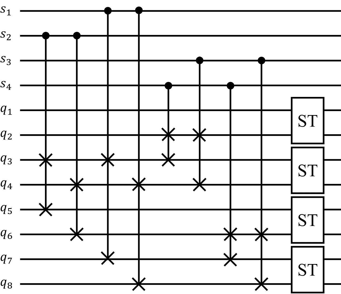
The simulated quantum circuit on IBM quantum cloud platform for 8-state Swap Test algorithm is given in Fig.(11), where q0q1q2q3q_{0}q_{1}q_{2}q_{3} are the auxiliary control qubits that corresponds to s1s2s3s4s_{1}s_{2}s_{3}s_{4}, q4q5q6q7q8q9q10q11q_{4}q_{5}q_{6}q_{7}q_{8}q_{9}q_{10}q_{11} are the initial states that corresponds to |ϕ1|ϕ2|ϕ3|ϕ4|ϕ5|ϕ6|ϕ7|ϕ8|\phi_{1}\rangle|\phi_{2}\rangle|\phi_{3}\rangle|\phi_{4}\rangle|\phi_{5}\rangle|\phi_{6}\rangle|\phi_{7}\rangle|\phi_{8}\rangle and q12q13q14q15q_{12}q_{13}q_{14}q_{15} are the result qubits of simple two-state Swap Test. The initial states q0q1q2q3q_{0}q_{1}q_{2}q_{3} are |+|+|+\left|+\right\rangle\left|+\right\rangle\left|+\right\rangle. Pair of normalized random numbers are generated by Python random package and the initial states q4q5q6q7q8q9q10q11q_{4}q_{5}q_{6}q_{7}q_{8}q_{9}q_{10}q_{11} in the experiment are |ϕ1=[0.0864,0.9963]|\phi_{1}\rangle=[0.0864,0.9963],|ϕ2=[0.8391,0.5440]|\phi_{2}\rangle=[0.8391,0.5440],|ϕ3=[0.2202,0.9755]|\phi_{3}\rangle=[0.2202,0.9755],|ϕ4=[0.5486,0.8361]|\phi_{4}\rangle=[0.5486,0.8361],|ϕ5=[0.2607,0.9654]|\phi_{5}\rangle=[0.2607,0.9654],|ϕ6=[0.4164,0.9091]|\phi_{6}\rangle=[0.4164,0.9091],|ϕ7=[0.9981,0.0609]|\phi_{7}\rangle=[0.9981,0.0609],|ϕ8=[0.4658,0.8849]|\phi_{8}\rangle=[0.4658,0.8849]. And the measurement results of this implementation through IBM Quantum Experience (QISKIT) are given in Fig.(12),with 8192 runs. Meanwhile, the measurement times of q0q1q2q3q12q13q14q15q_{0}q_{1}q_{2}q_{3}q_{12}q_{13}q_{14}q_{15} is shown in Appendix A.

Refer to caption
Figure 11: The circuit for 8-state Swap Test algorithm
Refer to caption
Figure 12: Result of implementation of 8-state Swap Test algorithm

The estimated overlap of |ϕi,|ϕj(i,j=1,2,,8;ij)\left|{\phi_{i}}\right\rangle,\left|{\phi_{j}}\right\rangle(i,j=1,2,...,8;i\neq j) can be obtained according to the relation of s1,s2,s3,s4s_{1},s_{2},s_{3},s_{4} and q1,q2,q3,q4,q5,q6,q7,q8q_{1},q_{2},q_{3},q_{4},q_{5},q_{6},q_{7},q_{8} in Table.2 and Appendix A. For example, s1,s2,s3,s4=|0010s_{1},s_{2},s_{3},s_{4}=\left|{0010}\right\rangle and s1,s2,s3,s4=|0011s_{1},s_{2},s_{3},s_{4}=\left|{0011}\right\rangle, the measurement result of q15q_{15} is related to estimate values of ϕ6|ϕ7\left\langle{\phi_{6}}\right|\left.{\phi_{7}}\right\rangle. After counting times of q15=|1q_{15}=\left|1\right\rangle t1=403t_{1}=403 and the times of q15=|0q_{15}=\left|0\right\rangle t0=601t_{0}=601, o^(|ϕ6,|ϕ7)=2t0t0+t11=0.4441\widehat{o}(|{\phi_{6}}\rangle,|{\phi_{7}}\rangle)={\frac{{2t_{0}}}{{t_{0}+t_{1}}}-1}=0.4441. The exact overlap of arbitrary two states o(|ϕi,|ϕj)o(\left|{\phi_{i}}\right\rangle,\left|{\phi_{j}}\right\rangle) and the estimated overlap of arbitrary two states o^(|ϕi,|ϕj)(i,j=1,2,,8;ij)\widehat{o}(\left|{\phi_{i}}\right\rangle,\left|{\phi_{j}}\right\rangle)(i,j=1,2,...,8;i\neq j) is shown in Table.(4).

o(|ϕ1,|ϕ2)o(\left|{\phi_{1}}\right\rangle,\left|{\phi_{2}}\right\rangle) o^(|ϕ1,|ϕ2)\widehat{o}(\left|{\phi_{1}}\right\rangle,\left|{\phi_{2}}\right\rangle) o(|ϕ1,|ϕ3)o(\left|{\phi_{1}}\right\rangle,\left|{\phi_{3}}\right\rangle) o^(|ϕ1,|ϕ3)\widehat{o}(\left|{\phi_{1}}\right\rangle,\left|{\phi_{3}}\right\rangle) o(|ϕ1,|ϕ4)o(\left|{\phi_{1}}\right\rangle,\left|{\phi_{4}}\right\rangle) o(|ϕ1,|ϕ4)o(\left|{\phi_{1}}\right\rangle,\left|{\phi_{4}}\right\rangle) o(|ϕ1,|ϕ5)o(\left|{\phi_{1}}\right\rangle,\left|{\phi_{5}}\right\rangle) o^(|ϕ1,|ϕ5)\widehat{o}(\left|{\phi_{1}}\right\rangle,\left|{\phi_{5}}\right\rangle)
0.3774 0.3959 0.9817 0.9880 0.7751 0.7590 0.9688 0.9610
o(|ϕ1,|ϕ6)o(\left|{\phi_{1}}\right\rangle,\left|{\phi_{6}}\right\rangle) o^(|ϕ1,|ϕ6)\widehat{o}(\left|{\phi_{1}}\right\rangle,\left|{\phi_{6}}\right\rangle) o(|ϕ1,|ϕ7)o(\left|{\phi_{1}}\right\rangle,\left|{\phi_{7}}\right\rangle) o(|ϕ1,|ϕ7)o(\left|{\phi_{1}}\right\rangle,\left|{\phi_{7}}\right\rangle) o(|ϕ1,|ϕ8)o(\left|{\phi_{1}}\right\rangle,\left|{\phi_{8}}\right\rangle) o^(|ϕ1,|ϕ8)\widehat{o}(\left|{\phi_{1}}\right\rangle,\left|{\phi_{8}}\right\rangle) o(|ϕ2,|ϕ3)o(\left|{\phi_{2}}\right\rangle,\left|{\phi_{3}}\right\rangle) o^(|ϕ2,|ϕ3)\widehat{o}(\left|{\phi_{2}}\right\rangle,\left|{\phi_{3}}\right\rangle)
0.8868 0.8949 0.0215 0.0009 0.8497 0.8658 0.5118 0.5697
o(|ϕ2,|ϕ4)o(\left|{\phi_{2}}\right\rangle,\left|{\phi_{4}}\right\rangle) o(|ϕ2,|ϕ4)o(\left|{\phi_{2}}\right\rangle,\left|{\phi_{4}}\right\rangle) o(|ϕ2,|ϕ5)o(\left|{\phi_{2}}\right\rangle,\left|{\phi_{5}}\right\rangle) o^(|ϕ2,|ϕ5)\widehat{o}(\left|{\phi_{2}}\right\rangle,\left|{\phi_{5}}\right\rangle) o(|ϕ2,|ϕ6)o(\left|{\phi_{2}}\right\rangle,\left|{\phi_{6}}\right\rangle) o^(|ϕ2,|ϕ6)\widehat{o}(\left|{\phi_{2}}\right\rangle,\left|{\phi_{6}}\right\rangle) o(|ϕ2,|ϕ7)o(\left|{\phi_{2}}\right\rangle,\left|{\phi_{7}}\right\rangle) o(|ϕ2,|ϕ7)o(\left|{\phi_{2}}\right\rangle,\left|{\phi_{7}}\right\rangle)
0.8374 0.8476 0.5533 0.5393 0.7123 0.6913 0.7581 0.7714
o(|ϕ2,|ϕ8)o(\left|{\phi_{2}}\right\rangle,\left|{\phi_{8}}\right\rangle) o^(|ϕ2,|ϕ8)\widehat{o}(\left|{\phi_{2}}\right\rangle,\left|{\phi_{8}}\right\rangle) o(|ϕ3,|ϕ4)o(\left|{\phi_{3}}\right\rangle,\left|{\phi_{4}}\right\rangle) o^(|ϕ3,|ϕ4)\widehat{o}(\left|{\phi_{3}}\right\rangle,\left|{\phi_{4}}\right\rangle) o(|ϕ3,|ϕ5)o(\left|{\phi_{3}}\right\rangle,\left|{\phi_{5}}\right\rangle) o(|ϕ3,|ϕ5)o(\left|{\phi_{3}}\right\rangle,\left|{\phi_{5}}\right\rangle) o(|ϕ3,|ϕ6)o(\left|{\phi_{3}}\right\rangle,\left|{\phi_{6}}\right\rangle) o^(|ϕ3,|ϕ6)\widehat{o}(\left|{\phi_{3}}\right\rangle,\left|{\phi_{6}}\right\rangle)
0.7607 0.7562 0.8768 0.8774 0.9982 0.9982 0.9574 0.9611
o(|ϕ3,|ϕ7)o(\left|{\phi_{3}}\right\rangle,\left|{\phi_{7}}\right\rangle) o^(|ϕ3,|ϕ7)\widehat{o}(\left|{\phi_{3}}\right\rangle,\left|{\phi_{7}}\right\rangle) o(|ϕ3,|ϕ8)o(\left|{\phi_{3}}\right\rangle,\left|{\phi_{8}}\right\rangle) o(|ϕ3,|ϕ8)o(\left|{\phi_{3}}\right\rangle,\left|{\phi_{8}}\right\rangle) o(|ϕ4,|ϕ5)o(\left|{\phi_{4}}\right\rangle,\left|{\phi_{5}}\right\rangle) o^(|ϕ4,|ϕ5)\widehat{o}(\left|{\phi_{4}}\right\rangle,\left|{\phi_{5}}\right\rangle) o(|ϕ4,|ϕ6)o(\left|{\phi_{4}}\right\rangle,\left|{\phi_{6}}\right\rangle) o^(|ϕ4,|ϕ6)\widehat{o}(\left|{\phi_{4}}\right\rangle,\left|{\phi_{6}}\right\rangle)
0.0779 0.1093 0.9325 0.9516 0.9028 0.9104 0.9773 0.9739
o(|ϕ4,|ϕ7)o(\left|{\phi_{4}}\right\rangle,\left|{\phi_{7}}\right\rangle) o(|ϕ4,|ϕ7)o(\left|{\phi_{4}}\right\rangle,\left|{\phi_{7}}\right\rangle) o(|ϕ4,|ϕ8)o(\left|{\phi_{4}}\right\rangle,\left|{\phi_{8}}\right\rangle) o^(|ϕ4,|ϕ8)\widehat{o}(\left|{\phi_{4}}\right\rangle,\left|{\phi_{8}}\right\rangle) o(|ϕ5,|ϕ6)o(\left|{\phi_{5}}\right\rangle,\left|{\phi_{6}}\right\rangle) o^(|ϕ5,|ϕ6)\widehat{o}(\left|{\phi_{5}}\right\rangle,\left|{\phi_{6}}\right\rangle) o(|ϕ5,|ϕ7)o(\left|{\phi_{5}}\right\rangle,\left|{\phi_{7}}\right\rangle) o(|ϕ5,|ϕ7)o(\left|{\phi_{5}}\right\rangle,\left|{\phi_{7}}\right\rangle)
0.3582 0.4323 0.9908 1.0 0.9727 0.9727 0.1017 0.0260
o(|ϕ5,|ϕ8)o(\left|{\phi_{5}}\right\rangle,\left|{\phi_{8}}\right\rangle) o^(|ϕ5,|ϕ8)\widehat{o}(\left|{\phi_{5}}\right\rangle,\left|{\phi_{8}}\right\rangle) o(|ϕ6,|ϕ7)o(\left|{\phi_{6}}\right\rangle,\left|{\phi_{7}}\right\rangle) o^(|ϕ6,|ϕ7)\widehat{o}(\left|{\phi_{6}}\right\rangle,\left|{\phi_{7}}\right\rangle) o(|ϕ6,|ϕ8)o(\left|{\phi_{6}}\right\rangle,\left|{\phi_{8}}\right\rangle) o(|ϕ6,|ϕ8)o(\left|{\phi_{6}}\right\rangle,\left|{\phi_{8}}\right\rangle) o(|ϕ7,|ϕ8)o(\left|{\phi_{7}}\right\rangle,\left|{\phi_{8}}\right\rangle) o^(|ϕ7,|ϕ8)\widehat{o}(\left|{\phi_{7}}\right\rangle,\left|{\phi_{8}}\right\rangle)
0.9519 0.9602 0.2218 0.1972 0.9970 0.9960 0.2691 0.2927
Table 4: The exact overlap value of arbitrary two states o(|ϕi,|ϕj)o(\left|{\phi_{i}}\right\rangle,\left|{\phi_{j}}\right\rangle) and the estimate overlap value of arbitrary two states o^(|ϕi,|ϕj)(i,j=1,2,,8;ij)\widehat{o}(\left|{\phi_{i}}\right\rangle,\left|{\phi_{j}}\right\rangle)(i,j=1,2,...,8;i\neq j)

The scatter diagram is shown in Fig.(13), where the estimate overlap value o^(|ϕi,|ϕj)\widehat{o}(\left|{\phi_{i}}\right\rangle,\left|{\phi_{j}}\right\rangle) is X-axis and the exact overlap value o(|ϕi,|ϕj)o(\left|{\phi_{i}}\right\rangle,\left|{\phi_{j}}\right\rangle) is Y-axis. It can be seen from Fig.(13) that most of the points fall near the diagonals of the picture, i.e. the line y=xy=x, indicating that the estimate overlap results are close to the exact overlap results.

Refer to caption
Figure 13: The relation of o(|ϕi,|ϕj)o(\left|{\phi_{i}}\right\rangle,\left|{\phi_{j}}\right\rangle) and o^(|ϕi,|ϕj)\widehat{o}(\left|{\phi_{i}}\right\rangle,\left|{\phi_{j}}\right\rangle)

9 data sets of the initial states D1,D2,D3,D4,D5,D6,D7,D8,D9D_{1},D_{2},D_{3},D_{4},D_{5},D_{6},D_{7},D_{8},D_{9} are generated by Python random package to be simulated in this experiment and their initial values are shown in Appendix B. And the scatter diagrams of estimated overlaps and exact overlaps of these 9 sets are shown in Fig.(14), where the estimated overlaps is X-axis and the exact overlaps is Y-axis. It can be seen from Fig.6 that most of the points fall near the diagonals of the picture, i.e., the line y=xy=x, indicating that the estimated overlaps are close to the exact overlaps.

Refer to caption
(a) D1D_{1}
Refer to caption
(b) D2D_{2}
Refer to caption
(c) D3D_{3}
Refer to caption
(d) D4D_{4}
Refer to caption
(e) D5D_{5}
Refer to caption
(f) D6D_{6}
Refer to caption
(g) D7D_{7}
Refer to caption
(h) D8D_{8}
Refer to caption
(i) D9D_{9}
Figure 14: The scatter diagrams of 9 groups quantum states

5 Analysis

In this section, we analyze the correctness and performance of our multi-state Swap Test algorithm in theory.

5.1 Correctness analysis

There is a transformation Un{\rm U}_{n}, which can take arbitrary unknown states |ϕ1,|ϕ2,|ϕn(n=2k(k>1))\left|{\phi_{1}}\right\rangle,\left|{\phi_{2}}\right\rangle,...\left|{\phi_{n}}\right\rangle(n=2^{k}(k>1)) as input states and 2(k1)2(k-1) |+\left|+\right\rangle as ancillaries. In Un{\rm U}_{n}, each pair |ϕ2i1,|ϕ2i(i=1,2,,n2)\left|{\phi_{2i-1}}\right\rangle,\left|{\phi_{2i}}\right\rangle(i=1,2,...,\frac{n}{2}) can be labeled by ancillaries |A(2i1)2i\left|{A_{(2i-1)2i}}\right\rangle by Lemma 4.1.

Lemma 4.1 Let n=2k(k>1)n=2^{k}(k>1), there exists a unitary Un{\rm U}_{n} that maps

Un:|+dni=1n|ϕi|yij+|1ij|Gij1ϕiϕjGij1++|mij|GijmϕiϕjGijm,U_{n}:|+\rangle^{d_{n}}\otimes_{i=1}^{n}|\phi_{i}\rangle\rightarrow|y_{ij}\rangle+|1_{ij}\rangle|G_{ij}^{1^{\prime}}\phi_{i}\phi_{j}G_{ij}^{1}\rangle+...+|m_{ij}\rangle|G_{ij}^{m^{\prime}}\phi_{i}\phi_{j}G_{ij}^{m}\rangle, (3)

where |ϕi,|ϕj|\phi_{i}\rangle,|\phi_{j}\rangle are arbitrary two input quantum states, and they are in adjacent quantum registers, i.e. in the quantum registers (q2i1,q2i),i{1,2,,n2}(q_{2i-1},q_{2i}),i\in\{1,2,...,{n\over 2}\}. |Gij,|Gij,|yij|G_{ij}^{\prime}\rangle,|G_{ij}\rangle,|y_{ij}\rangle are garbage states which is irrelevant to our target states, i.e. |ϕi,|ϕj|\phi_{i}\rangle,|\phi_{j}\rangle. |1ij,,|mij|1_{ij}\rangle,...,|m_{ij}\rangle represents the state in the first dnd_{n} quantum registers. That means we can get all pairs |ϕi|ϕj,ij|\phi_{i}\rangle|\phi_{j}\rangle,i\neq j by measuring the specific quantum registers (q2i1,q2i),i{1,2,,n2}(q_{2i-1},q_{2i}),i\in\{1,2,...,{n\over 2}\} in the quantum circuit.

Constructive proof of Lemma 4.1 According to scientific induction, we assume that Lemma 4.1 is correct at first. Let the nn quantum registers divided into 4 groups Q11=(q1,,qn/4)Q_{1}^{1}=(q_{1},...,q_{n/4}),Q12=(qn/4+1,,qn/2)Q_{1}^{2}=(q_{n/4+1},...,q_{n/2}), Q13=(qn/2+1,,q3n/4)Q_{1}^{3}=(q_{n/2+1},...,q_{3n/4}),Q14=(q3n/4+1,,qn)Q_{1}^{4}=(q_{3n/4+1},...,q_{n}). Furthermore, we get 4 quantum states |Φ11=|ϕ1ϕn/4|\Phi_{1}^{1}\rangle=|\phi_{1}...\phi_{n/4}\rangle,|Φ12=|ϕn/4+1,,ϕn/2|\Phi_{1}^{2}\rangle=|\phi_{n/4+1},...,\phi_{n/2}\rangle, |Φ13=|ϕn/2+1,,ϕ3n/4|\Phi_{1}^{3}\rangle=|\phi_{n/2+1},...,\phi_{3n/4}\rangle,|Φ14=|ϕ3n/4+1,,ϕn|\Phi_{1}^{4}\rangle=|\phi_{3n/4+1},...,\phi_{n}\rangle. Applying Un/2{\rm U}_{n/2} to (Q11,Q12)(Q_{1}^{1},Q_{1}^{2}) and (Q13,Q14)(Q_{1}^{3},Q_{1}^{4}) respectively, we can get all pairs of input states |Φ11Φ12|\Phi_{1}^{1}\Phi_{1}^{2}\rangle, i.e. |ϕ1,,|ϕn/2|\phi_{1}\rangle,...,|\phi_{n/2}\rangle, and the same is true for the other Un/2{\rm U}_{n/2}. If we apply a unitary U4{\rm U}_{4} on (Q11,Q12,Q13,Q14)(Q_{1}^{1},Q_{1}^{2},Q_{1}^{3},Q_{1}^{4}) before the Un/2{\rm U}_{n/2}, we will get all pairs of input states |ϕ1,,|ϕn|\phi_{1}\rangle,...,|\phi_{n}\rangle. For example, we want to get a pair |ϕaϕb,a[1,n4],b[n2+1,3n4]|\phi_{a}\phi_{b}\rangle,a\in[1,{n\over 4}],b\in[{n\over 2}+1,{3n\over 4}]. |Φ11Φ13|\Phi_{1}^{1}\Phi_{1}^{3}\rangle will be stored in (Q11,Q12)(Q_{1}^{1},Q_{1}^{2}) if the ancillary qubits of U4{\rm U}_{4} is |01|01\rangle, and the pair |ϕaϕb|\phi_{a}\phi_{b}\rangle might be measured after Un/2{\rm U}_{n/2}.

Similarly, the correctness of Un/2{\rm U}_{n/2} can be provide by using Un/4{\rm U}_{n/4} and U4{\rm U}_{4}, and so on. Finally, the correctness of U4{\rm U}_{4} is shown in Table.1. So Lemma 4.1 is proved. For the case that nn cannot be written in the form of 2k2^{k}, we can add 2kn2^{k}-n copy of any input state as the rest input.

So far, we have obtained all pairs of nn input quantum states, and can get each pair exactly according to the measurement results of auxiliary qubits. Therefore, we only need to apply the Swap Test in all specific registers (q1,q2),,(qn1,qn)(q_{1},q_{2}),...,(q_{n-1},q_{n}) to get the overlap between two input quantum states. As shown in Figure(16), the measurement results of 2(k1)2(k-1) auxiliaries determine the quantum state in each quantum register uniquely. Because it has been proved that all pairs of input quantum states have the opportunity to be measured in specific registers, all overlap estimates can be obtained after enough measurements.

5.2 Performance analysis

In this section, we compare our scheme and the scheme Swap Test for an arbitrary number of quantum states given by Gitiaux(referred to as SAN scheme later in this article).

5.2.1 Precision

The precision of estimation is determined by the occurrences of each overlap with the total number of runs given, thus we can use this value ,denoted by m to represent the precision. For the SAN scheme, only one measurement can be obtained each time the quantum circuit is run. Therefore, in the case of n=2kn=2^{k} quantum state inputs, if the count of quantum circuit is run for NN times, each overlap is estimated to occur 2Nn(n1)2N\over{n(n-1)} times in average, i.e., m1=2Nn(n1)m_{1}={2N\over{n(n-1)}}. For our scheme, one execution contains n2n\over 2 Swap Test operations. So in the same case, we have the precision m2=Nn1m_{2}={N\over{n-1}},which means higher precision.

Refer to caption
Figure 15: The precision for different schemes(expressed in terms of ratio)

Fig.(15) shows the ratio of the average precision of our scheme with respect to SAN. Taking the number of the SAN scheme m1m_{1} as the standard, it can be seen that with the increase of the circuits depth, the ratio between the new scheme and SAN scheme m2m1m_{2}\over m_{1} increases gradually, indicating that our precision advantage becomes gradually more pronounced as the circuit depth increases.The stepwise growth is due to the fact that we must apply such kk that 2k1<n2k2^{k-1}<n\leq 2^{k}. It should be noted that if the probability of occurrence of each quantum state is taken into account, the estimation of different overlaps will have different precision.This is because the number of recurrences of different pairs varies according to the table, which means that some pairs may occur more frequently. However, this only depends on the artificial choices we make when coding, and the total effect does not have a large impact as the number increases.

5.2.2 Space complexity

The space complexity of Un{\rm U}_{n} consists of the count of CSWAP gates and the number of ancillaries, where n=2kn=2^{k} and k=log2nk=log_{2}n. First of all, we notice that the count of CSWAP gates cnc_{n} follows the recursive relation:

cn=2cn/2+n2c_{n}=2c_{n/2}+{n\over 2} (4)

where the first term comes from two Un/2{\rm U}_{n/2} and the second term comes from a U4{\rm U}_{4}. The general term formula cn=nkc_{n}=nk can be obtained by simplifying the sequence relation. If considering the CSWAP gates come from the following Swap Test operation, we havecn=n(k+12)c_{n}=n(k+{1\over 2}). Similarly, for SAN scheme, we can get the general term formula for the number of CSWAP gates cn=3(n1)c_{n}^{\prime}=3(n-1), which is shown in the right panel of Fig.(16). Furthermore, if we concentrate on the count of CSWAP gates, the complexity of Un{\rm U}_{n} in our scheme isO(nlogn)O(n\log n) and in SAN scheme is O(n){\rm O}(n). Obviously, our scheme uses more CSWAP gates and has higher complexity than the SAN scheme.

As for the number of ancillaries, we have the relation:

dn=dn1+2d_{n}=d_{n-1}+2 (5)

which means each time the number of input quantum states is doubled, 2 additional auxiliaries are required. It can be rewritten as dn=2k2d_{n}=2k-2, and the general term formula for SAN scheme the number of ancillaries is dn=3k3d_{n}^{\prime}=3k-3. Obviously, our scheme uses fewer ancillaries than the SAN scheme, and both complexities are O(logn){\rm O}(\log n). The relationship between the number of auxiliaries and the number of input quantum states (assuming that all input quantum states are single quantum states) is shown in Figure(18). As shown in the left panel. the red line and the green line represent our scheme and SAN scheme respectively. It can be seen that the number of auxiliaries required by our new scheme is less than that of the SAN scheme.

Refer to caption
Figure 16: The complexity of two schemes. The left panel shows the count of ancillaries of two schemes, and the complexities of CSWAP gates is shown in the right panel.

If we consider the additional auxiliaries brought by the subsequent Swap Test of the two Swap Test schemes, we can reduce it by using the Swap Test circuit optimization scheme mentioned in section 2 to reduce the auxiliaries through classical calculation. At this time, the total number of qubits required by our scheme will be less than that required by the SAN scheme, which means less resource consumption.

To sum up, our scheme provides a better estimation under the same count of circuit runs. At the same time, the number of auxiliaries required in our scheme is less than that of the SAN scheme. Although the complexity of the count of CSWAP gates in the SAN scheme is O(n){\rm O}(n) which is less than that in our scheme O(nlogn)O(n\log n), When the circuits run, they are processed in parallel and do not affect the total time, so we trade a certain space cost for the desired time cost.

6 Summary

In this paper, we propose a new scheme for estimating overlap between all pair of input quantum states. Given arbitrary number of input quantum states |ϕ1,|ϕn|\phi_{1}\rangle,...|\phi_{n}\rangle. the scheme provide a way to calculate the overlap |ϕi|ϕj|2|\langle\phi_{i}|\phi_{j}\rangle|^{2} for all pair of input quantum states where i<ji,j1,2,,ni<j\ i,j\in{1,2,...,n}.

Our scheme is based on the scheme given by [19]. The basic principle is we concentrate a unitary Un{\rm U}_{n} according to nn input quantum states |ϕ1,,|ϕn|\phi_{1}\rangle,...,|\phi_{n}\rangle, which is used to obtain a specific superposition state, so that we can get all pairs of input quantum states at a specific position (q2n1,q2n),n1,2,,n2(q_{2n-1},q_{2n}),n\in{1,2,...,{n\over 2}}. In order to decode the measurement results, we use O(logn)O(\log n) auxiliary qubits, their measurement results reveal what the quantum state in the register is. Finally, the results are obtained by performing Swap Test on these positions to estimate the value of overlap between each pair. A total of O(nlogn)O(n\log n) CSWAP gates are used in the quantum circuit. We carry out experiments on IBM cloud platform, and give a exact analysis to verify the correctness of our scheme. At the same time, we analyze the complexity and accuracy of our scheme. Compared with the original scheme [19], our scheme uses fewer auxiliary qubits and has higher accuracy, but the line depth (the number of CSWAP gates) will be higher than the original scheme. Therefore, if it is possible to find a way to reduce the use of cswap gates, the performance of the scheme will be further improved.

This work was supported in part by the 2019 National Social Science Foundation Art Major Project, Network Culture Security Research, under Grant 19zd12, in part by the High-Quality and Cutting-Edge Disciplines Construction Project for Universities in Beijing (Internet Information, Communication University of China), and in part by the Fundamental Research Funds for the Central Universities, and by Equipment Pre-research Field Fund under Grant 61403110320.

References

References

  • [1] Shor P W 1982 International Journal of exact Physics 21 467-488
  • [2] Deutsch D 1985 Proceedings of the Royal Society A Mathematical 400 97-117
  • [3] Shor, Peter W 1999 SIAM Review 26 1484-1509
  • [4] Grover L K 1996 Proceedings of the twenty-eighth annual ACM symposium on Theory of computing (STOC96) 212-219
  • [5] Lloyd S 1996 Science 273 1073-1078
  • [6] Farhi E , Goldstone J , Gutmann S , et al, 2000 Physics
  • [7] Harrow A W , Hassidim A , Lloyd S 2009 Physical Review Letters 103 150502
  • [8] Jordan S (https://quantumalgorithmzoo.org/ (Accessed: 2020-11-07))
  • [9] Aimeur E , Zekrifa D M S , Gambs S 2006 Proceedings of the 19th international conference on Advances in Artificial Intelligence: Canadian Society for Computational Studies of Intelligence(Springer-Verlag) 431-42
  • [10] Chuang I , Gottesman D 2001 SIAM Review (arXiv:quant-ph/0105032)
  • [11] Garcia-Escartin J C , Chamorro-Posada P 2013 Physical Review A 87 239-257
  • [12] Cincio L , Y Subaşı, Sornborger A T , et al, 2018 New Journal of Physics 20 113022
  • [13] Fanizza M , Rosati M , Skotiniotis M , et al, 2020 Physical review letters 124 060503
  • [14] Chabaud U , Diamanti E , Markham D , et al, 2018 Physical Review A 98 062318
  • [15] Linke N M , Johri S , Figgatt C , et al, 2017 APS March Meeting(American Physical Society)
  • [16] Lloyd S , Mohseni M , Rebentrost P 2013 (arXiv:1307.0411)
  • [17] Wiebe N , Kapoor A , Svore K 2014 Quantum Information &\& Computation 15 318-358
  • [18] V Havlíček, AD Córcoles, Temme K , et al, 2019 Nature 567 209-212
  • [19] Schuld Maria,Sinayskiy Ilya ,et al, 2015 (arXiv:1409.3097)
  • [20] Kang Min-Sung, Heo Jino,et al 2019 Scientific Reports9 (1) 6167
  • [21] Gitiaux X, Morris I , Emelianenko M , et al, 2021 (arXiv:2110.13261)

Appendix

A

|q0q1q2q3q12q13q14q15|q_{0}q_{1}q_{2}q_{3}q_{12}q_{13}q_{14}q_{15}\rangle counts |q0q1q2q3q12q13q14q15|q_{0}q_{1}q_{2}q_{3}q_{12}q_{13}q_{14}q_{15}\rangle counts |q0q1q2q3q12q13q14q15|q_{0}q_{1}q_{2}q_{3}q_{12}q_{13}q_{14}q_{15}\rangle counts
|10110000|10110000\rangle 398 |01100101|01100101\rangle 38 |00111000|00111000\rangle 38
|01010000|01010000\rangle 235 |00110000|00110000\rangle 207 |00000100|00000100\rangle 7
|10011000|10011000\rangle 245 |11011100|11011100\rangle 30 |01000110|01000110\rangle 1
|00110100|00110100\rangle 60 |11101100|11101100\rangle 3 |00001011|00001011\rangle 2
|01001000|01001000\rangle 83 |10100100|10100100\rangle 55 |10000010|10000010\rangle 4
|00000000|00000000\rangle 221 |01110101|01110101\rangle 31 |01111000|01111000\rangle 22
|10011100|10011100\rangle 36 |00110001|00110001\rangle 148 |01101000|01101000\rangle 9
|11100010|11100010\rangle 10 |00110101|00110101\rangle 34 |00100011|00100011\rangle 4
|11100000|11100000\rangle 389 |10000101|10000101\rangle 9 |10101000|10101000\rangle 29
|01100000|01100000\rangle 256 |11010100|11010100\rangle 32 |01001011|01001011\rangle 6
|10100000|10100000\rangle 388 |00101101|00101101\rangle 4 |00111100|00111100\rangle 5
|10000100|10000100\rangle 116 |11100001|11100001\rangle 19 |10111010|10111010\rangle 1
|01010100|01010100\rangle 45 |01110011|01110011\rangle 3 |00010110|00010110\rangle 19
|01000001|01000001\rangle 114 |10001001|10001001\rangle 4 |10000001|10000001\rangle 18
|11010000|11010000\rangle 238 |01000010|01000010\rangle 18 |01000011|01000011\rangle 6
|11101000|11101000\rangle 29 |00100100|00100100\rangle 62 |00110111|00110111\rangle 2
|00010010|00010010\rangle 220 |00100101|00100101\rangle 35 |01111001|01111001\rangle 4
|01110100|01110100\rangle 73 |00111001|00111001\rangle 16 |01000100|01000100\rangle 3
|10001100|10001100\rangle 43 |11110001|11110001\rangle 20 |00000101|00000101\rangle 10
|00101000|00101000\rangle 26 |10110100|10110100\rangle 57 |11110101|11110101\rangle 1
|11111010|11111010\rangle 44 |11001100|11001100\rangle 49 |00001100|00001100\rangle 9
|01010010|01010010\rangle 189 |00100010|00100010\rangle 4 |11010001|11010001\rangle 4
|11111010|11111010\rangle 4 |01100001|01100001\rangle 88 |11000110|11000110\rangle 8
|11111000|11111000\rangle 32 |10100010|10100010\rangle 19 |10011001|10011001\rangle 2
|11000000|11000000\rangle 200 |01010110|01010110\rangle 33 |01111110|01111110\rangle 1
|10101010|10101010\rangle 1 |00111101|00111101\rangle 4 |10100001|10100001\rangle 6
|00010000|00010000\rangle 238 |10110010|10110010\rangle 18 |11000001|11000001\rangle 6
|00100001|00100001\rangle 131 |10010100|10010100\rangle 30 |01011000|01011000\rangle 4
|11011000|11011000\rangle 218 |01011010|01011010\rangle 5 |00011010|00011010\rangle 3
|10001000|10001000\rangle 93 |00101001|00101001\rangle 18 |10000110|10000110\rangle 1
|00100000|00100000\rangle 189 |01101001|01101001\rangle 2 |10111001|10111001\rangle 1
|11100100|11100100\rangle 54 |01100100|01100100\rangle 69 |01000101|01000101\rangle 1
|00000001|00000001\rangle 126 |01110110|01110110\rangle 2 |00001101|00001101\rangle 3
|11000100|11000100\rangle 121 |00000010|00000010\rangle 2 |11001010|11001010\rangle 6
|01000000|01000000\rangle 195 |10110001|10110001\rangle 12 |01011110|01011110\rangle 1
|00001000|00001000\rangle 99 |11100110|11100110\rangle 2 |11110010|11110010\rangle 2
|11110000|11110000\rangle 413 |00010100|00010100\rangle 18 |11011001|11011001\rangle 4
|11001000|11001000\rangle 104 |10111000|10111000\rangle 26 |11100101|11100101\rangle 3
|01110001|01110001\rangle 109 |01100010|01100010\rangle 6 |00101111|00101111\rangle 1
|01001001|01001001\rangle 49 |01110010|01110010\rangle 7 |11111100|11111100\rangle 2
|10010000|10010000\rangle 231 |00101100|00101100\rangle 7 |00101011|00101011\rangle 1
|10000000|10000000\rangle 234 |10111100|10111100\rangle 5 |01001100|01001100\rangle 1
|01110000|01110000\rangle 252 |01101100|01101100\rangle 8 |01001101|01001101\rangle 1
|00001001|00001001\rangle 56 |01100011|01100011\rangle 3 |00110011|00110011\rangle 4
|11000010|11000010\rangle 13 |01111101|01111101\rangle 2 |10001110|10001110\rangle 1
|10110110|10110110\rangle 3 |10001101|10001101\rangle 2 |11000101|11000101\rangle 1
|11001001|11001001\rangle 1 |01001010|01001010\rangle 4 |10001010|10001010\rangle 1
|00010111|00010111\rangle 1 |01101010|01101010\rangle 1 |00001010|00001010\rangle 2
|11001110|11001110\rangle 2 |00111110|00111110\rangle 1 |00110010|00110010\rangle 2
|10100110|10100110\rangle 2 |10101100|10101100\rangle 1 |11101001|11101001\rangle 1
|00100111|00100111\rangle 1 |01111100|01111100\rangle 3 |11011110|11011110\rangle 1
|01110111|01110111\rangle 1 |11111101|11111101\rangle 1 |10010001|10010001\rangle 2
|10110101|10110101\rangle 1 |11111001|11111001\rangle 2 |10010101|10010101\rangle 1
|10100101|10100101\rangle 1 |10100011|10100011\rangle 1 |11011101|11011101\rangle 1
Table 5: The counts of different measurement result of ancillary qubits q0,q1,q2,q3,q12,q13,q14,q15q_{0},q_{1},q_{2},q_{3},q_{12},q_{13},q_{14},q_{15}

B

D1:D_{1}: D2:D_{2}: D3:D_{3}:
|ϕ1=[0.1340,0.9910]|ϕ2=[0.5666,0.8240]|ϕ3=[0.1262,0.9920]|ϕ4=[0.2899,0.9571]|ϕ5=[0.9746,0.2238]|ϕ6=[0.4602,0.8878]|ϕ7=[0.9813,0.1926]|ϕ8=[0.9695,0.2452]\begin{array}[]{l}|\phi_{1}\rangle=[0.1340,0.9910]\\ |\phi_{2}\rangle=[0.5666,0.8240]\\ |\phi_{3}\rangle=[0.1262,0.9920]\\ |\phi_{4}\rangle=[0.2899,0.9571]\\ |\phi_{5}\rangle=[0.9746,0.2238]\\ |\phi_{6}\rangle=[0.4602,0.8878]\\ |\phi_{7}\rangle=[0.9813,0.1926]\\ |\phi_{8}\rangle=[0.9695,0.2452]\\ \end{array} |ϕ1=[0.9697,0.2443]|ϕ2=[0.8136,0.5814]|ϕ3=[0.2681,0.9634]|ϕ4=[0.1963,0.9806]|ϕ5=[0.5862,0.8102]|ϕ6=[0.2324,0.9726]|ϕ7=[0.9565,0.2917]|ϕ8=[0.5461,0.8377]\begin{array}[]{l}|\phi_{1}\rangle=[0.9697,0.2443]\\ |\phi_{2}\rangle=[0.8136,0.5814]\\ |\phi_{3}\rangle=[0.2681,0.9634]\\ |\phi_{4}\rangle=[0.1963,0.9806]\\ |\phi_{5}\rangle=[0.5862,0.8102]\\ |\phi_{6}\rangle=[0.2324,0.9726]\\ |\phi_{7}\rangle=[0.9565,0.2917]\\ |\phi_{8}\rangle=[0.5461,0.8377]\\ \end{array} |ϕ1=[0.8240,0.5665]|ϕ2=[0.0398,0.9992]|ϕ3=[0.3343,0.9425]|ϕ4=[0.4898,0.8719]|ϕ5=[0.8140,0.5808]|ϕ6=[0.7047,0.7095]|ϕ7=[0.3366,0.9416]|ϕ8=[0.6131,0.7900]\begin{array}[]{l}|\phi_{1}\rangle=[0.8240,0.5665]\\ |\phi_{2}\rangle=[0.0398,0.9992]\\ |\phi_{3}\rangle=[0.3343,0.9425]\\ |\phi_{4}\rangle=[0.4898,0.8719]\\ |\phi_{5}\rangle=[0.8140,0.5808]\\ |\phi_{6}\rangle=[0.7047,0.7095]\\ |\phi_{7}\rangle=[0.3366,0.9416]\\ |\phi_{8}\rangle=[0.6131,0.7900]\\ \end{array}
D4:D_{4}: D5:D_{5}: D6:D_{6}:
|ϕ1=[0.2945,0.9557]|ϕ2=[0.6896,0.7242]|ϕ3=[0.1983,0.9801]|ϕ4=[0.3120,0.9501]|ϕ5=[0.6402,0.7682]|ϕ6=[0.0190,0.9998]|ϕ7=[0.6453,0.7639]|ϕ8=[0.7724,0.6351]\begin{array}[]{l}|\phi_{1}\rangle=[0.2945,0.9557]\\ |\phi_{2}\rangle=[0.6896,0.7242]\\ |\phi_{3}\rangle=[0.1983,0.9801]\\ |\phi_{4}\rangle=[0.3120,0.9501]\\ |\phi_{5}\rangle=[0.6402,0.7682]\\ |\phi_{6}\rangle=[0.0190,0.9998]\\ |\phi_{7}\rangle=[0.6453,0.7639]\\ |\phi_{8}\rangle=[0.7724,0.6351]\\ \end{array} |ϕ1=[0.4298,0.9029]|ϕ2=[0.5133,0.8582]|ϕ3=[0.3321,0.9432]|ϕ4=[0.9703,0.2419]|ϕ5=[0.1018,0.9948]|ϕ6=[0.1415,0.9899]|ϕ7=[0.3026,0.9531]|ϕ8=[0.1908,0.9816]\begin{array}[]{l}|\phi_{1}\rangle=[0.4298,0.9029]\\ |\phi_{2}\rangle=[0.5133,0.8582]\\ |\phi_{3}\rangle=[0.3321,0.9432]\\ |\phi_{4}\rangle=[0.9703,0.2419]\\ |\phi_{5}\rangle=[0.1018,0.9948]\\ |\phi_{6}\rangle=[0.1415,0.9899]\\ |\phi_{7}\rangle=[0.3026,0.9531]\\ |\phi_{8}\rangle=[0.1908,0.9816]\\ \end{array} |ϕ1=[0.0089,1.0000]|ϕ2=[0.1810,0.9835]|ϕ3=[0.6282,0.7780]|ϕ4=[0.6501,0.7599]|ϕ5=[0.4055,0.9141]|ϕ6=[0.4306,0.9026]|ϕ7=[0.1430,0.9897]|ϕ8=[0.2031,0.9792]\begin{array}[]{l}|\phi_{1}\rangle=[0.0089,1.0000]\\ |\phi_{2}\rangle=[0.1810,0.9835]\\ |\phi_{3}\rangle=[0.6282,0.7780]\\ |\phi_{4}\rangle=[0.6501,0.7599]\\ |\phi_{5}\rangle=[0.4055,0.9141]\\ |\phi_{6}\rangle=[0.4306,0.9026]\\ |\phi_{7}\rangle=[0.1430,0.9897]\\ |\phi_{8}\rangle=[0.2031,0.9792]\\ \end{array}
D7:D_{7}: D8:D_{8}: D9:D_{9}:
|ϕ1=[0.5632,0.8263]|ϕ2=[0.1064,0.9943]|ϕ3=[0.9086,0.4176]|ϕ4=[0.0576,0.9983]|ϕ5=[0.3325,0.9431]|ϕ6=[0.0025,1.0000]|ϕ7=[0.0900,0.9960]|ϕ8=[0.7227,0.6912]\begin{array}[]{l}|\phi_{1}\rangle=[0.5632,0.8263]\\ |\phi_{2}\rangle=[0.1064,0.9943]\\ |\phi_{3}\rangle=[0.9086,0.4176]\\ |\phi_{4}\rangle=[0.0576,0.9983]\\ |\phi_{5}\rangle=[0.3325,0.9431]\\ |\phi_{6}\rangle=[0.0025,1.0000]\\ |\phi_{7}\rangle=[0.0900,0.9960]\\ |\phi_{8}\rangle=[0.7227,0.6912]\\ \end{array} |ϕ1=[0.8502,0.5265]|ϕ2=[0.1541,0.9881]|ϕ3=[0.3624,0.9320]|ϕ4=[0.3696,0.9292]|ϕ5=[0.8279,0.5608]|ϕ6=[0.1571,0.9876]|ϕ7=[0.4334,0.9012]|ϕ8=[0.7817,0.6237]\begin{array}[]{l}|\phi_{1}\rangle=[0.8502,0.5265]\\ |\phi_{2}\rangle=[0.1541,0.9881]\\ |\phi_{3}\rangle=[0.3624,0.9320]\\ |\phi_{4}\rangle=[0.3696,0.9292]\\ |\phi_{5}\rangle=[0.8279,0.5608]\\ |\phi_{6}\rangle=[0.1571,0.9876]\\ |\phi_{7}\rangle=[0.4334,0.9012]\\ |\phi_{8}\rangle=[0.7817,0.6237]\\ \end{array} |ϕ1=[0.7207,0.6932]|ϕ2=[0.0995,0.9950]|ϕ3=[0.1926,0.9813]|ϕ4=[0.7677,0.6408]|ϕ5=[0.2066,0.9784]|ϕ6=[0.0124,0.9999]|ϕ7=[0.2994,0.9541]|ϕ8=[0.84579,0.5335]\begin{array}[]{l}|\phi_{1}\rangle=[0.7207,0.6932]\\ |\phi_{2}\rangle=[0.0995,0.9950]\\ |\phi_{3}\rangle=[0.1926,0.9813]\\ |\phi_{4}\rangle=[0.7677,0.6408]\\ |\phi_{5}\rangle=[0.2066,0.9784]\\ |\phi_{6}\rangle=[0.0124,0.9999]\\ |\phi_{7}\rangle=[0.2994,0.9541]\\ |\phi_{8}\rangle=[0.84579,0.5335]\\ \end{array}
Table 6: The initial states for D1,D2,D3,D4,D5,D6,D7,D8,D9D_{1},D_{2},D_{3},D_{4},D_{5},D_{6},D_{7},D_{8},D_{9}