Multi-Sample based Contrastive Loss for Top-k Recommendation
Abstract
The top-k recommendation is a fundamental task in recommendation systems which is generally learned by comparing positive and negative pairs. The Contrastive Loss (CL) is the key in contrastive learning that has received more attention recently and we find it is well suited for top-k recommendations. However, it is a problem that CL treats the importance of the positive and negative samples as the same. On the one hand, CL faces the imbalance problem of one positive sample and many negative samples. On the other hand, positive items are so few in sparser datasets that their importance should be emphasized. Moreover, the other important issue is that the sparse positive items are still not sufficiently utilized in recommendations. So we propose a new data augmentation method by using multiple positive items (or samples) simultaneously with the CL loss function. Therefore, we propose a Multi-Sample based Contrastive Loss (MSCL) function which solves the two problems by balancing the importance of positive and negative samples and data augmentation. And based on the graph convolution network (GCN) method, experimental results demonstrate the state-of-the-art performance of MSCL. The proposed MSCL is simple and can be applied in many methods. We will release our code on GitHub upon the acceptance.
Index Terms:
contrastive loss, recommendation system, data augmentation, graph convolution networkI Introduction
Recommendation systems have become an important research field which aims to solve the information overload problem in the information explosion era. The recommendation system is widely used in many fields, such as e-commerce [1, 2], life services[3, 4], social networks[5, 6], entertainment[7, 8], and it becomes one of the important technologies in the information age. The top-k recommendation is the basic problem of recommendation systems which learns the users’ preferences through their historical interaction records. Then it recommends top k items to the users that they may like.
Deep learning based top-k recommendation algorithms significantly improve the recommendation performance and become the mainstream research direction in recent years, especially the collaborative filtering based methods. These existing algorithms extract advanced semantic features and perform complex feature interactions by employing MLP[9], CNN[10], RNN[11], attention mechanism[12, 13], etc. The user-item interaction is naturally viewed as a bipartite graph. Graph convolutional networks (GCN) based methods are increasingly integrated with recommendation systems, such as NGCF[14], LR-GCCF[15], LightGCN[16], DGCF[17]. GCN based methods aggregate features of neighbors as well as higher-order neighbors to obtain better feature representations of users and items and the performance has been further improved.
In contrast to the rapid development of the recommendation methods, the loss function has rarely been improved. Bayesian Personalized Ranking (BPR) [18] is a widely used loss function for the top-k recommendation, which maximizes the distance between positive and negative pairs. Recently, the contrastive loss (CL) function has yielded excellent results in several fields under the contrastive learning framework [19, 20, 21, 22, 23, 24]. In CL, all non-positive samples in the same batch are used as negative samples, while BPR uses one or several negative samples by random sampling. They all learn through a contrastive process, so BPR loss can also be seen as a kind of contrastive loss. BPR samples one or several true negative samples, while CL directly treats non-positive items within the same training batch as negative samples. CL can obtain a large number of negative samples simply and quickly while BPR utilizes a small number of samples and requires additional sampling time.

However, the importance of positive and negative samples should be treated differently by CL. (1) CL uses one positive sample and -1 negative samples where is the batch size, typically 1024, 2048, etc. Thus the imbalance problem or different importance of the one positive sample and negative samples should be tackled. (2) The count of positive samples is very small thus recommendation systems facing the sparsity problem. Intuitively, the sparser the dataset, the fewer positive samples, and the more important the positive samples should be, relative to the many negative samples. Therefore, positive and negative samples should be treated differently according to the above two reasons.
Another issue we concern about is the insufficient use of positive samples in the top-k recommendation. As mentioned before, there are very limited positive items of each user in the recommendation system. How to make full use of the existing positive samples is a key problem. Data augmentation methods help to solve this problem. Data augmentation methods in the recommendation system are generally based on graph structures, such as edge or node dropout, masking features, random walk and so on. The potential of the combined use of positive samples is not exploited.
To solve the above problems, we propose a new CL based loss function and the basic idea is shown in Fig. 1. For the first problem, we distinguished their different importance by adjusting the weights of positive and negative samples. The hyperparameter is the weight of the positive samples which represents their importance. To make better use of positive items, we propose a new data augmentation method by using multiple positive samples simultaneously. This data augmentation makes better use of positive samples for the training space can be expanded because of different combinations of multiple positive samples. In the original situations, how many items the user has interacted with can be interpreted as how many cases the user can encounter. By a random combination of multiple items, the user can encounter more cases, thus expanding the training space. Moreover, this data augmentation can be used for many other types of data, not just graph data.
In summary, we propose a contrastive loss function based on multiple (positive and negative) samples, which is named as Multi-Sample based Contrastive Loss (MSCL). The main contributions of this paper are summarized as follows:
-
•
We propose a simple but effective loss function, MSCL, which improves the contrastive loss to make it suitable for the recommendation system. MSCL can be applied to many models of recommendation system and is much better than the traditional BPR loss.
-
•
The MSCL function distinguishes the importance of positive and negative samples by weighting. It helps to address the imbalance problem of positive and negative samples as well as to enhance the importance of positive samples in sparser datasets.
-
•
We propose a new data augmentation method by using multiple positive samples simultaneously which makes better use of the positive samples.
-
•
Experimental results demonstrate the state-of-the-art performance and many other advantages, such as broad applicability, high training efficiency. MSCL is suitable for the top-k recommendation, and it makes the simple and basic MF more competitive.
The rest of this paper is organized as follows: In Section II, related works are briefly reviewed. To verify the effectiveness of MSCL, we design sLightGCN_MSCL which combines MSCL with the best baseline as our method in Section III. Experiments and discussions are shown in Section IV. Section V discusses the advantages of MSCL with more experiments. Conclusions are drawn in Section VI.
II Related work
In this section, we briefly review related works: the contrastive loss and graph data augmentation methods. Differences between ours and existing works are also presented.
II-A Contrastive Loss (CL)
The contrastive loss has become an excellent tool in unsupervised representation learning. It aims to maximize the similarities of positive pairs and minimize that of negative pairs [19, 20, 25, 26, 27]. The contrastive loss function is widely used for many kinds of data, such as images, text, audio, graphs, etc. It has been applied in the field of recommendation[28, 29].
Broadly speaking, functions that use pairwise contrastive learning processes are contrastive loss functions which have many forms. BPR and triplet loss are the basic contrast-based and widely used loss functions. BPR [18] loss aims to maximize the distance between positive pair and negative pair, which is proposed for the ranking task and widely used in the top-k recommendation. Triplet loss [30, 31, 32] can be used to train samples with small differences, especially for human faces. The samples are triplets (anchor, positive, negative). The triplet loss is calculated by optimizing the distance between the anchor and positive samples to be smaller than the distance between the anchor and negative samples.
However, they employ limited pairs of samples. Contrastive loss functions based on multiple pairs of samples are more efficient which contain Multi-class N-pair loss, InfoNCE loss, Non-Parametric Softmax Classifier, NT-Xent loss. Multi-class N-pair loss [33] is proposed from a deep metric learning perspective, which greatly improves the triplet loss by jointly pushing out multiple negative samples at each update. InfoNCE loss [34, 35, 36] is proposed by maximizing a lower bound on mutual information based on Noise-Contrastive Estimation. Non-Parametric Softmax Classifier [37] is presented by maximizing distinction between instances via a novel non-parametric softmax formulation in an unsupervised feature learning approach. They come from different fields and formula derivation but share a similar form. NT-Xent loss (the normalized temperature-scaled cross entropy loss) [19, 24] is proposed on these bases, but with the minor difference that the denominator does not contain positive samples. All of them are widely used in contrastive learning framework and always obtain the state-of-the-art results.
II-B Graph Data Augmentation
The user-item interaction records in recommendation systems are naturally viewed as bipartite graphs. Graph-based data augmentation is widely used and studied in graph contrastive learning, which contains both traditional subgraph sampling methods and recently proposed methods [38, 39, 28, 24, 40, 41]. User and item are inherently linked and dependent on each other in the user-item bipartite graph. Data augmentation for GCN is also challenging due to the complex, non-Euclidean structure of the graph, and few works study the data augmentation of graphs. Therefore, graph data augmentation must be tightly integrated with the graph rather than replicating the methods used in Computer Vision and Natural Language Processing domains.
Graph data augmentation conforms to the basic assumptions of graph data processing. Node dropping assumes that edge vertex missing does not alter semantics. Edge perturbation is considered to improve the robustness of the semantics against connectivity changes. Masking node features enhance semantic robustness by losing some attributes for each node. Subgraphs assume that local structure can hint the complete semantics [24].
The graph augmentation can be divided into two types, feature-space augmentations and structure-space augmentations: (1) feature-space augmentations are realized by modifying initial node features, such as masking features or adding Gaussian noise, and (2) structure-space augmentations operate on graph structure by adding or removing nodes or edges (edge perturbation), sub-sampling or subgraphs by random walk, or generating different views using shortest distances or diffusion matrices [40].
Recently, Zhu et al. [41] proposes adaptive graph augmentation to design augmentation schemes that tend to keep important structures and attributes unchanged while the unimportant links and features are perturbed. Zhao et al. [42] utilizes a neural edge predictor to predict likely edges for graph augmentation to improve node classification performance. For top-k recommendations, the latest work, SGL [28], uses three operators on the graph structure, namely node dropout, edge dropout and random walk. And experimental results show that the edge dropout performs the best.
II-C Differences with Existing Works
Differences with existing CL functions: Many works are done just using the CL function in the contrastive Learning framework. SGL in the recommendation system employs a multi-tasking mechanism with joint use of CL and BPR. Despite some improvements are proposed on CL, such as soft contrastive loss [43], debiased contrastive loss [44], they all treat the weights of the positive sample and negative samples as the same. And the problem of imbalanced positive and negative samples is still not be concerned. More importantly, how to adapt CL to recommendation systems is a new topic worth investigating, especially to emphasize the importance of positive samples on sparser datasets. Thus, the proposed importance-aware CL is different from the previous works.
Differences with existing graph data augmentation: Existing graph data augmentations in the recommendation system are common methods in the graph field. How to make full use of the limited positive samples to obtain better results, especially for the recommendation system is an important task and challenge for data augmentation. We randomly sampled a fixed number within one-hop neighbors which is not the same as random dropout or subgraph by random walk on multiple hops. More importantly, our method is a structure-space based augmentation, and traditional structure-space based methods are generally work in the aggregation process of GCNs. The traditional augmented data are used one by one under the same loss which is a serial approach. We use multiple positive samples at the same time and combine them explicitly with the loss function which is a parallel way for better constraints.
III Methodology
We designed a method named as sLightGCN_MSCL which combine MSCL with a strong baseline as shown in Fig. 2. to verify the effectiveness of the proposed loss function. It should be noted that our approach is model-agnostic and can be applied to many methods of recommendation systems. In this section, we first briefly describe the basic methods LightGCN, then focus on the MSCL function, and finally analyze the time complexity.

III-A Basic Method
Recently, graph related methods have shown excellent performances, which treat user-item interactions as graph structures and adopt graph convolution network. Combined with collaborative filtering, NGCF [14], LR-GCCF [15], LightGCN [16], etc. are excellent models for top-k recommendation.
LightGCN is the state-of-the-art method and is introduced here as our main baseline. This model includes only the most essential component in GCN - neighborhood aggregation - for collaborative filtering which is much easier to implement and train and gains substantial improvements. Then neighborhood aggregation is defined as follows:
| (1) |
| (2) |
where denote the user and the item in the user-item graph, respectively denote embeddings of of the -th layer. Specially, represents the initialized latent vector; and represent the set of the neighbors of target and , relatively. The final embedings of users and items are:
| (3) |
| (4) |
where is the numbers of layers; denotes the importance of the -th layer embedding, and they can be treated as a hyper-parameter to be tuned manually, or as a model parameter to be optimized automatically. Following the original paper of LightGCN, the mean of embeddings from all layers are adopted as the final embeddings, that is =1/(+1).
LightGCN-single, a variant of LightGCN are also proposed in the paper, where only the -th embeddings, , are used as final embeddings. This variant, instead of the original LightGCN, is used here for its better performance and is named sLightGCN for short.
The BPR loss is used for training in LightGCN. We present it here for comparison with MSCL.
| (5) |
where is the logistic sigmoid function.
III-B Multi-Sample based Contrastive Loss (MSCL)
III-B1 The Basic Contrastive Loss (CL)
Refer to some recent works [19, 24], we use the NT-Xent as the original contrastive loss function and then adapt it to the recommendation field.
The NT-Xent is:
| (6) |
where , and , means the embeddings of sample in a minibatch, is the batch size, denotes the temperature parameter. To fit the recommendation domain, we rewrite it as :
| (7) |
| (8) |
where is a training batch; , is the set of users and items, respectively; means the positive sample of target user , and is the set of negative samples. is the cosine similarity of the pair based on their embeddings. We follow the sampling strategy used in [19, 24] that the other non-positive samples in the same batch are seen as negative samples.
III-B2 Importance-aware CL (ICL)
In the basic contrastive loss, the minus sign is preceded by one positive sample, followed by the sum of negative samples which results in imbalance problems. In addition, emphasizing the importance of positive samples on sparser datasets is also a problem we want to address. These two problems can be solved together by weighting, an effective and common practice. The importance of positive and negative samples can be adjusted which helps to better backpropagate and make the training more effective. We name the modified CL as importance-aware CL, which is:
| (9) |
where is a hyperparameter and .
When , the is the same as . Because problems in the analysis are inevitable, is not optimal in general. When , it means that -1 negative samples need more weights and relatively more losses to be optimized. When , it means that the positive samples need to be given more attention, and it may be because there are too few positive items for users in the recommendation system. The weighting method is simple yet effective in adapting to a variety of datasets.
III-B3 Multiple Positive Samples based CL (MCL)
To address the problem that positive samples are insufficiently used, we propose a new data augmentation method that uses multiple positive samples simultaneously. We propose a multi-path based method to use multiple positive samples under the supervision of CL function. The conventional approach is to use a random batch of data and a loss function to form a learning path after the model is computed. We extend this idea by randomly sampling positive samples to form paths. The target user is optimized by positive samples. The final loss is the sum of loss functions which is calculated simply and effectively. Thus, the multiple positive samples based CL is:
| (10) |
where is a hyperparameter which is the number of used positive samples.
This data augmentation comes with many benefits. (1) We keep the same training process of MSCL and the original one, but the difference is theof samples used for each training. Suppose the user has positive samples, there are (Combination formula) possible cases by random sampling for the user at each training time in the original way. MSCL uses positive samples simultaneously for the user, so there are possible cases for each training. Therefore, the positive samples greatly increase the cases that users can encounter. This makes augmentation and better usage of the existing positive items. (2) Positive and negative samples form a comparison, thus the expanded positive samples also enlarge the comparable cases. (3) Furthermore, we integrate this augmentation with the loss function explicitly in a parallel way to facilitate more and better constraint and backpropagation for the user. (4) And this data augmentation method can be widely applied to graph data as well as various other types of data.
III-B4 Multi-Sample based CL (MSCL)
We have elaborated on our two improvements, ICL and MCL. These two improvements are proposed from different perspectives. Combining them together can solve the two problems for the top-k recommendation. In this case, multiple positive samples and many negative samples are used at the same time. Therefore, we term it as Multi-Sample based Contrastive Loss, which is defined as follows:
| (11) |
Their combination forms a logic for this paper: using multiple (positive and negative) samples and solve the problems that exist in them. The proposed function is simple and effective. Two hyperparameters are introduced, but they are easy to tune.
III-C Model Prediction
The model prediction is defined as the inner product of the user and item final embeddings:
| (12) |
Based on this prediction, the top-k most similar items are recommended to the user.
The proposed MSCL is used for model training, and the method is named as sLightGCN_MSCL. MSCL replaces the BPR loss which is used in the original LightGCN. Except for the proposed loss function, our method remains the same as the LightGCN. The L2 regularization for all parameters is also used following LightGCN, and it is omitted here for clarity.
III-D Complexity Analyses
In this subsection, we analyze the complexity of sLightGCN_MSCL following SGL [28]. Since sLightGCN_MSCL does not introduce trainable parameters and there is no change of model prediction, the spatial complexity and the time complexity of the model inference are the same as LightGCN. The complexity of sLightGCN_MSCL can be divided into two parts, that of sLightGCN and MSCL, and they are , , where is the edge in the user-item interaction graph, denote the number of GCN layers, the number of epochs, the number of multiple positive samples, and denote the embedding size, the batch size, respectively. For comparison, that of the BPR loss is .
In fact, the overall amount of calculation is significantly reduced because the number of training epoch is substantially reduced due to better convergence performance as shown in training efficiency in section V. MSCL is times larger than the computational cost of BPR, but this is a simple inner product which is directly accelerated by matrix operations through the GPU. Therefore, there is no significant increase in training time in each epoch as can be seen in section V.
IV Experiments
We first introduce the basic information related to the experiments, such as datasets, evaluation metrics, and hyper-parameter settings. sLightGCN_MSCL is compared with many strong baselines. We conduct ablation studies to verify the effectiveness of the proposed improvements. The main hyper-parameters of sLightGCN_MSCL are discussed in detail.
IV-A Datasets
To evaluate the effectiveness of MSCL, we conduct experiments on three benchmark datasets: Yelp2018 [16, 28], Amazon-Book [16, 28], and Alibaba-iFashion [28, 2].
Yelp2018: Yelp2018 is adopted from the 2018 edition of the Yelp challenge. The local businesses like restaurants and bars are viewed as the items.
Amazon-book: Amazon-review is a widely used dataset for product recommendation and Amazon-book from the collection is selected.
Alibaba-iFashion: Alibaba-iFashion is a large and rich dataset for Fashion Outfit recommendation. 300k users and all their interactions over the fashion outfits are randomly sampled by SGL [28]. It is quite sparse, which is a significant difference from the first two datasets.
| Dataset | Users | Items | Interactions | Density |
|---|---|---|---|---|
| Yelp2018 | 31,668 | 38,048 | 1,561,406 | 0.00130 |
| Amazon-Book | 52,643 | 91,599 | 2,984,108 | 0.00062 |
| Alibaba-iFashion | 300,000 | 81,614 | 1,607,813 | 0.00007 |
Three datasets vary significantly in domains, size, and sparsity. The statics of the processed datasets are summarized in Table I. For comparison purposes, we directly use the split data provided in SGL[28].
| Method | Yelp2018 | Amazon-Book | Alibaba-iFashion | |||
| Recall | NDCG | Recall | NDCG | Recall | NDCG | |
| MF | 0.0441 | 0.0353 | 0.0329 | 0.0249 | 0.1020 | 0.0474 |
| NGCF | 0.0579 | 0.0477 | 0.0344 | 0.0263 | 0.1043 | 0.0486 |
| LR-GCCF | 0.0591 | 0.0485 | 0.0378 | 0.0292 | 0.1110 | 0.0529 |
| LightGCN | 0.0639 | 0.0525 | 0.0411 | 0.0315 | 0.1078 | 0.0507 |
| sLightGCN | 0.0649 | 0.0525 | 0.0469 | 0.0363 | 0.1160 | 0.0553 |
| Mult-VAE | 0.0584 | 0.0450 | 0.0407 | 0.0315 | 0.1041 | 0.0497 |
| SGL | 0.0675 | 0.0555 | 0.0478 | 0.0379 | 0.1126 | 0.0538 |
| LightGCN_MSCL(ours) | 0.0681 | 0.0564 | 0.0500 | 0.0391 | 0.1144 | 0.0546 |
| sLightGCN_MSCL(ours) | 0.0691 | 0.0568 | 0.0580 | 0.0466 | 0.1201 | 0.0578 |
IV-B Evaluation Metrics
Following NGCF, LightGCN, and SGL [14, 16, 28], two widely used evaluation metrics, Recall@K and NDCG@K where K=20, are used to evaluate the performance of top-k recommendation. Recall measures the number of items that the user likes in the test data that has been successfully predicted in the top-k ranking list. NDCG considers the positions of the items and higher scores are given if the items are ranked higher. It is a metric about ranking and thus is important for the top-k recommendation. The larger the values, the better the performance for both metrics.
IV-C Hyper-parameter Settings
We implement our proposed method on top of the official code of LightGCN111https://github. com/gusye1234/LightGCN-PyTorch based with Pytorch. We replace the loss function and follow LightGCN’s settings as much as possible. The embedding size is fixed to 64 and the default batch size is 2048 for all models. The learning rate and L2 regularization coefficients are chosen by grid search in the range of and . These are hyper-parameters of the original LightGCN. We adjust hyper-parameters of MSCL, and , in the ranges , , respectively. And is 0.1 or 0.2 usually. The weight is adjust in [0.4,0.7].
IV-D Compared Methods
To demonstrate the performance of our method, we select many strong baselines for comparison. NGCF [14], LR-GCCF [15], LightGCN [16] are the competing baselines with GCN of top-k recommendation recently which having shown to outperform several methods including GC-MC [45], PinSage [46], NeuMF [9] since the previous works [14, 16, 15]. The latest methods, SGL [28], is also selected which is a self-supervised based method. In addition, the basic method and the variable autoencoder-based methods, MF and Mult-VAE, are compared.
MF: This is a traditional method based on matrix factorization which is based only on the embeddings of users and items, namely and .
NGCF [14]: NGCF integrates the bipartite graph structure into the embedding process based on the graph convolutional network. It explicitly exploits the collaborative signal in the form of high-order connectivities by propagating embeddings on the graph structure.
LR-GCCF [15]: This method enhances the recommendation performance with less complexity by removing the non-linearity. The final embeddings are the same as NGCF.
LightGCN and sLightGCN [16]: LightGCN is the state-of-the-art GCN based collaborative filtering model, and sLightGCN is a variant. They are described in detail in Section III.
Mult-VAE [47]: Mult-VAE extends variational autoencoders (VAEs) to collaborative filtering and uses a multinomial likelihood for the data distribution. Besides, it introduces an additional regularization parameter for optimization. It can be seen as a special case of self-supervised learning(SSL) for recommendation.
SGL [28]: SGL is the latest baseline for top-k recommendations. It introduces self-supervised learning into the recommendation system based on the contrastive learning framework. It is implemented on LightGCN and uses a multi-task approach that unites the contrastive loss and the BPR loss function. SGL mainly benefits from graph contrastive learning to reinforce user and item representations. Following the paper, the edge drop based SGL achieving the best performance are adopted here.
| Loss | Importance-aware | Multi-positive samples | Yelp2018 | Amazon-Book | Alibaba-iFashion | |||
|---|---|---|---|---|---|---|---|---|
| Recall | NDCG | Recall | NDCG | Recall | NDCG | |||
| CL | 0.0655 | 0.0541 | 0.0480 | 0.0399 | 0.1152 | 0.0556 | ||
| ICL | ✓ | 0.0668 | 0.0548 | 0.0544 | 0.0437 | 0.1165 | 0.0558 | |
| MCL | ✓ | 0.0677 | 0.0559 | 0.0516 | 0.0425 | 0.1184 | 0.0573 | |
| MSCL | ✓ | ✓ | 0.0691 | 0.0568 | 0.0580 | 0.0466 | 0.1201 | 0.0578 |
IV-E Performance Comparison
The performance comparison on the three datasets is shown in Table II. The best results are shown in bold while underlined scores are the second best. We follow the experimental results of SGL [28], except for MF, LR-GCCF, and our methods. After statistical analysis, the standard deviations on Recall and NDCG are not big than under different initialization seeds. We have the following observations:
MF is the most basic and simplest method and performs the worst. NGCF, LR-GCCF, and LightGCN are GCN based methods. NGCF achieved improvements relative to MF by introducing the GCN method into top-k recommendations, especially on the Yelp2008 dataset. LR-GCCF, LightGCN and sLightGCN can be seen as improvements of NGCF. Their performances are better than NGCF, and these results are consistent with the performance in the original paper. These three methods show the significant role of graph convolution methods in recommendation systems. LightGCN is the strongest baseline and becomes the basis for subsequent methods, such as SGL and our method. LightGCN removes the nonlinear activation layer and learning parameters making the model more applicable to recommendation systems rather than simply employing GCN which illustrates that the GCN method should be modified to fit the recommendation system.
Mult-VAE and SGL are methods that belong to self-supervised learning (SSL). The results of Mult-VAE are generally better than NGCF, indicating that the variational auto-encoder based method and self-supervised learning is competitive for recommendation. The results of SGL show that it has a clear boost compared with LightGCN and suboptimal results are obtained on two datasets which demonstrates the advancement of contrastive learning methods.
The proposed sLightGCN_MSCL is the best among all methods. LightGCN_MSCL is also listed as a variant of our method, which is also superior to other methods. Compared to the latest and best method SGL, the improvements of sLightGCN_MSCL on Yelp2018, Amazon-Book, and Alibaba-iFashion are 2.37%, 21.34%, 6.67% on Recall, 2.34%, 22.96%, 7.43% on NDCG, respectively. SGL uses CL and BPR jointly in the multi-task learning approach without exploiting the potential of CL. Our approach is simpler and consumes less time which can be seen in Training Efficiency in Section V. This shows the correctness of improving CL.
IV-F Ablation Study
MSCL combines two components, the different importance of positive and negative samples and the use of multiple positive samples. ICL, MCL denote importance-aware CL and multiple positive samples based CL respectively. They are shown in Equations (8)-(10).
IV-F1 The effectiveness of the two components
Detailed ablation studies demonstrate the effectiveness of our two components as shown in Table III. The comparison of CL and ICL, MCL and MSCL show the effectiveness of adding weights to distinguish the importance of positive and negative samples. The comparison of CL and MCL, ICL and MSCL illustrate the effectiveness of data augmentation based on multiple positive samples. All the results, the two evaluation metrics on three datasets in these four comparison groups, in Table III consistently demonstrate the effectiveness of the two components.
Besides, we find the three datasets perform differently on the two components. Amazon-Book benefits more from adding weights to distinguish the importance while the other two datasets improve more significantly on multiple positive samples. This shows that the proposed two components are effective, but perform differently depending on the dataset.
IV-F2 Detailed analysis about the role of multiple positive samples
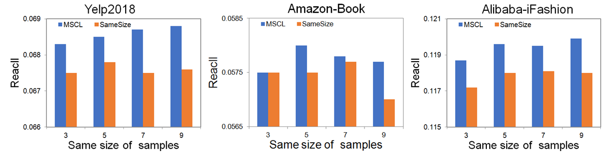
More comparisons in training tend to yield better results such as a large batch size. Our data augmentation approach of using multiple positive samples also increases the count of comparisons in each epoch. Therefore, one of the reasons for the good performance of multiple positive samples also involves more comparisons. However, we want to show that our proposed approach makes better use of positive samples, except for thecountof comparisons. Experiments with the same number of comparisons need to be done to exclude this factor. We expand the batch size of ICL to * because a user is compared with * items in MSCL, where is the training batch size.
The results are shown in Fig. 3. Our method consistently outperforms the latter on the three datasets. Overall, the performance of the same batch size peaks and falls back as batch size increases, especially on Amazon-Book. And they are significantly worse than the performances of multiple positive samples when =9. Yelp2018 and Alibaba-iFashion have the same trend of change in Fig. 3 which is different from that of Amazon-Book. This is consistent with the above observation in Table III that Yelp2018 and Alibaba-iFashion behave differently from Amazon-Book. In summary, the combination of multiple positive samples makes better use of the limited number of positive samples.


IV-G Discussion
IV-G1 Impact of the Weight
We adjust the weight and the results are shown in Fig. 4. The results show that both weighting methods achieve better results relative to unweighted when is 0.5. The first two datasets both obtain the best performance at 0.45, while Alibaba-iFashion reaches the best at 0.60. The main reason for this difference is that Alibaba-iFashion is the sparsest dataset and has few positive samples of users. Each user has 49.3, 56.7, and 6.4 positive items on average on the three datasets, respectively. For Yelp2018 and Amazon-Book, the imbalance problem is the main issue, and thus thousands of negative samples do require relatively more weights to learn better. Compared to the other two datasets, positive items of Alibaba-iFashion are so few that positive samples should be more important and given more weight. This illustrates that the first two datasets benefit mainly from solving the imbalance problem and the last dataset benefits mainly from increasing the importance of a limited number of positive samples. It also demonstrates that the weighting approach can solve these two both problems to balance the importance of positive and negative samples and can adapt to different datasets, despite its simplicity.
IV-G2 Impact of the number of positive samples
Both MSCL and MCL are able to illustrate the role of multiple positive samples and the results are shown in Fig. 5. All the results of MSCL and MCL with multiple positive samples are significantly better than those with only one positive sample on the left. So the proposed data augmentation method does make better use of the positive samples. MSCL and MCL have the same tend on the three datasets. As the number of positive samples increases, MSCL and MCL start with a significant improvement, and then change flatly. It can be seen from Fig. 5 that about 5 or 7 is appropriate, and more positive samples tend to be slightly better.
Besides, it is consistent with expectations that the results in the left bottom of each dataset in Fig. 5 are the worst which do not incorporate any improvements. It also shows that all results of MSCL are better than the MCL with the same number of positive samples, demonstrating the effectiveness of the importance-aware method.
V Advantages of MSCL
| Method | Yelp2018 | Amazon-Book | Alibaba-iFashion | |||
|---|---|---|---|---|---|---|
| Recall | NDCG | Recall | NDCG | Recall | NDCG | |
| MF_BPR | 0.0441 | 0.0353 | 0.0329 | 0.0249 | 0.1020 | 0.0474 |
| MF_MSCL | 0.0657(48.98%) | 0.0538(52.41%) | 0.0478(45.29%) | 0.0369(48.19%) | 0.1185(16.18%) | 0.0576(21.52%) |
| NGCF_BPR | 0.0579 | 0.0477 | 0.0344 | 0.0263 | 0.1043 | 0.0486 |
| NGCF_MSCL | 0.0655(13.13%) | 0.0538(12.79%) | 0.0481(39.83%) | 0.0375(42.59%) | 0.1152(10.45%) | 0.0565(16.26%) |
| LR-GCCF_BPR | 0.0591 | 0.0485 | 0.0378 | 0.0292 | 0.1072 | 0.0507 |
| LR-GCCF_MSCL | 0.0658(11.34%) | 0.0543(11.96%) | 0.0465(23.02%) | 0.0360(23.29%) | 0.1119(4.38%) | 0.0533(5.13%) |
| sLightGCN_BPR | 0.0649 | 0.0525 | 0.0469 | 0.0363 | 0.1160 | 0.0553 |
| sLightGCN_MSCL | 0.0691(6.47%) | 0.0568(8.19%) | 0.0580(23.67%) | 0.0466(28.37%) | 0.1201(3.53%) | 0.0578(4.52%) |

We have obtained optimal results of MSCL by the method sLightGCN_MSCL on top-k recommendation. We focus on the proposed loss function MSCL in this section. MSCL is simple and easy to implement, but it also has many other advantages, such as applicability, more suitable for the top-k recommendation, high training efficiency. In addition, MSCL improves the simplest and most basic model MF significantly making it more valuable for applications. Finally, as an extension, we verify that the problems and the improvements of this paper are also generalizable to multiple samples based BPR function.
V-A Applicability of MSCL
To show the applicability of MSCL, we apply it to many methods and compare it with the BPR loss, and methods with these two loss are named as “*-MSCL”, “*-BPR”.
The results are shown in Table IV, and the percentage of improvements relative to BPR are also presented. MSCL-based methods outperform the BPR-based methods on all results on the three datasets, and have significant improvements on MF, NGCF and LR-GCCF. sLightGCN_MSCL consistently obtains the best results on all datasets and has desirable improvements. In particular, the improvement on the Amazon-Book dataset is still about 25%.
Furthermore, MF is the most fundamental method just based on embeddings in the recommendation field, and many methods can be seen as developments of MF. Theoretically, MSCL is suitable for all embedding based methods. Thus, the effectiveness of MF shows that MSCL can be widely used in recommendation systems. The above experimental results and analysis show that our proposed MSCL is model-agnostic and widely adaptable.

V-B Suitable for the Top-k Recommendation
We think that MSCL is more suitable for the Top-k recommendation task. This can be illustrated by theoretical analysis and experimental results.
Theoretically, MSCL is compared with the loss function BPR. The common goal of both BPR and MSCL is to learn better feature representation by comparing between positive and negative samples. BPR uses a limited number of comparisons, usually one or several while MSCL employ thousands. Moreover, MSCL improves the quality of comparison by distinguishing the importance of positive and negative samples and makes better use of the few positive samples. MSCL makes the similarities between positive and negative samples more accurate through more and better comparisons. The top-k recommendation is a ranking task, and BPR is proposed specifically for ranking tasks. MSCL outperforms BPR in terms of theoretical and experimental results. Therefore, MSCL could get better ranking results and makes more sense for top-k recommendations.
Experimentally, the improvement of the evaluation metric NDCG is more obvious. NDCG is a ranking related metric which is more meaningful for ranking and top-k recommendation task compared to Recall. The following two observations support us well: (1) In Table IV, we found that the NDCG boost generally more than Recall. On average, the improvements are 19.98%, 32.95%, 8.64% on Recall while that are 21.34%, 35.61%, 11.86% on NDCG for the three datasets respectively. This shows the superiority of MSCL for top-k recommendation on different methods. (2) Fig. 6 shows the more significant improvement of MSCL over BPR on NDCG compared to Recall with different . This shows that the ranking performance of NDCG is consistently higher than Recall even as changes.
V-C The Improvement of MSCL on MF
The performance of MF_MSCL is particularly noteworthy in Table IV.
(1) MF_MSCL gains the most significant improvement, among all MSCL-based versus BPR-based methods. The results are even better than those of all BPR-based methods, sLightGCN_BPR included. It indicates MSCL with the most basic and simple method is significantly better than excellent methods recently proposed, even the state-of-the-art GCN methods. Thus, to some extent, a good loss function works better than new models.
(2) In addition, we find that the results MF_MSCL are also competitive. They are close to or better than that of NGCF_MSCL and LR-GCCF_MSCL on all datasets, and are close to sLightGCN_MSCL on the Alibaba-iFashion dataset. This indicates that MSCL is also effective in directly optimizing embeddings without a complex model, such as GCN.
These observations also indicate that MSCL can achieve competitive results in the simplest baseline, which is also consistent with the latest research Graph-MLP [48]. Graph-MLP indicates that it is sufficient for learning discriminative node representations only by MLP and graph based CL, without the complex GCN. Compared with Graph-MLP, MF_MSCL is more concise and simple. It is based only on embeddings and improved CL functions, which is still effective even without MLP. Graph-MLP does not optimize the CL loss function which is what we do, this shows the great potential of MSCL.
Three other points need to be highlighted. (1) As the most basic and simple method, MF_MSCL can be widely used in various tasks of recommendation systems, not only the top-k tasks. The applicability of MSCL is best illustrated by MF_MSCL. (2) MF_MSCL also has other advantages of MSCL presented in this section, such as being more suitable for top-k recommendation and fast convergence. (3) Importantly, it is valuable for applications with high space and time requirements or industrial applications at a large scale.
V-D Training Efficiency
| BPR | MSCL | MSCL | MSCL | MSCL | |
|---|---|---|---|---|---|
| M=1 | M=5 | M=10 | M=15 | ||
| Yelp2018 | 13 | 12 | 15 | 19 | 22 |
| Amazon-Book | 64 | 61 | 65 | 71 | 77 |
| Alibaba-iFashion | 17 | 16 | 19 | 22 | 25 |
The training efficiency of MSCL is also significantly improved as shown in Fig. 7. Because of the large difference in loss values, following LightGCN, SGL, the test performance on three datasets are used to show the convergence speed. In terms of the number of training epochs required to achieve optimal performance, more than 900 epochs are required for BPR, while MSCL achieves the best performance at 46, 3, and 90 epochs on the three datasets respectively. BPR requires too many epochs for convergence while MSCL converges earlier, so we adopt the same number of epoch as MACL for comparison.
For the first two datasets, MSCL converges directly to the high values approximating the final performance with slight fluctuations while BPR converges slowly at lower values. On the third dataset, it is slightly more difficult to converge due to the sparsity of the dataset. MSCL converges sharply by about 5 epochs to the value that approximates the final performance. This all shows that MSCL has a fast convergence capability. The training efficiency is improved at least tens of times on different datasets in terms of train epochs as mentioned before. The main reason for the high training efficiency is that multiple samples are learned at the same time as demonstrated in [38].
Moreover, in terms of actual training time, MSCL does not significantly increase the training time per epoch. Table V shows the average time consumption in each epoch in seconds. MSCL takes less time than BPR when one positive sample is used as shown in the first two columns of the table. Because BPR requires negative sampling while MSCL needs not and the computation with multiple negative samples is accelerated by the GPU. When the number of positive samples increases by 1, the average time increased on the three data sets is 0.8s. Such time consumption is completely negligible. When =5, MSCL and BPR consume the same time, but the performance is much better than BPR. Relative to the latest SGL [28] based on the contrastive learning framework, it takes about 3.7x larger than LightGCN while ours is about 1.5 times of LightGCN.
The above analyses demonstrate that MSCL has remarkable improvement in convergence speed and training efficiency than BPR. And there is no significant increase in time consumption per epoch, which is an advantage over SGL in terms of performance and time consumption.
V-E Multi-Sample based BPR Loss (MSBPR)
| BPR | MSBPR | MSCL | ||
|---|---|---|---|---|
| Yelp2018 | Recall | 0.0649 | 0.0670 | 0.0691 |
| NDCG | 0.0525 | 0.0552 | 0.0568 | |
| Amazon-Book | Recall | 0.0469 | 0.0458 | 0.058 |
| NDCG | 0.0363 | 0.0371 | 0.0466 | |
| Alibaba-iFashion | Recall | 0.1160 | 0.1172 | 0.1201 |
| NDCG | 0.0553 | 0.0564 | 0.0578 |
The proposed MSCL combines ICL and MCL aiming to solve the problem of different importance of positive and negative samples and insufficient use of positive samples. The problems and solutions are also fit for BPR. Therefore, we modify the loss function of the multi-sample based BPR in the same way and present the MSBPR function. In this case, the same sampling method of MSCL is used by MSBPR. The formula of MSBPR is as follows:
| (13) | ||||
where is the logistic sigmoid. We use instead of by drawing on comparative learning because the based approach doesn’t work.
The results are shown in Table VI, and the baseline is sLightGCN. With the only exception in all results that the recall of MSBPR is worse than BPR on Amazon-Book, the overall MSBPR-based methods are better than BPR. It shows that our proposed idea can be extended to BPR and other pair-wise based loss functions. In addition, we find that MSCL works better than MSBPR, especially on the Amazon-Book dataset, which shows the superiority of the CL function again and the correctness of improving CL in this paper. Therefore, MSCL is better than BPR and MSBPR in the field of recommendation systems.
VI Conclusion
In this paper, we propose MSCL function for the multi-sample based recommendation systems. We distinguish the different importance of positive and negative samples and propose a new data augmentation method to make better use of positive samples. MSCL is simple but obtains optimal results. More importantly, it has the advantages of wide applicability to various models, suitability for the top-k recommendation, and high training efficiency. MSCL makes simple and basic MF more valuable for industrial applications. These advantages make MSCL more competitive for top-k recommendation tasks.
This work represents an initial attempt to exploit improved CL for the recommendation. We believe that other improvements based on CL are an important direction. The two problems, the different importance of positive and negative samples, insufficient use of positive samples, are still valuable and deserve to be studied in depth. The proposed MSCL has the potential to be extended to graph-related fields as well as other fields.
References
- [1] Sanshi Yu, Zhuoxuan Jiang, Dongdong Chen, Shanshan Feng, Dongsheng Li, Qi Liu, and Jinfeng Yi. Leveraging tripartite interaction information from live stream e-commerce for improving product recommendation. In KDD, pages 3886–3894. ACM, 2021.
- [2] Wen Chen, Pipei Huang, Jiaming Xu, Xin Guo, Cheng Guo, Fei Sun, Chao Li, Andreas Pfadler, Huan Zhao, and Binqiang Zhao. POG: personalized outfit generation for fashion recommendation at alibaba ifashion. In KDD, pages 2662–2670. ACM, 2019.
- [3] Zhenxing Xu, Ling Chen, Yimeng Dai, and Gencai Chen. A dynamic topic model and matrix factorization-based travel recommendation method exploiting ubiquitous data. IEEE Transactions on Multimedia, 19(8):1933–1945, 2017.
- [4] Yuxia Wu, Ke Li, Guoshuai Zhao, and Xueming QIAN. Personalized long- and short-term preference learning for next poi recommendation. IEEE Transactions on Knowledge and Data Engineering, pages 1–1, 2020.
- [5] Shangrong Huang, Jian Zhang, Lei Wang, and Xian-Sheng Hua. Social friend recommendation based on multiple network correlation. IEEE Transactions on Multimedia, 18(2):287–299, 2016.
- [6] Guoshuai Zhao, Xiaojiang Lei, Xueming Qian, and Tao Mei. Exploring users’ internal influence from reviews for social recommendation. IEEE Transactions on Multimedia, 21(3):771–781, 2019.
- [7] Xusong Chen, Dong Liu, Zhiwei Xiong, and Zheng-Jun Zha. Learning and fusing multiple user interest representations for micro-video and movie recommendations. IEEE Transactions on Multimedia, 23:484–496, 2021.
- [8] Guoshuai Zhao, Zhidan Liu, Yulu Chao, and Xueming Qian. Caper: Context-aware personalized emoji recommendation. IEEE Transactions on Knowledge and Data Engineering, 33(9):3160–3172, 2021.
- [9] Xiangnan He, Lizi Liao, Hanwang Zhang, Liqiang Nie, Xia Hu, and Tat-Seng Chua. Neural collaborative filtering. In WWW, pages 173–182. ACM, 2017.
- [10] Xiangnan He, Xiaoyu Du, Xiang Wang, Feng Tian, Jinhui Tang, and Tat-Seng Chua. Outer product-based neural collaborative filtering. In IJCAI, pages 2227–2233. ijcai.org, 2018.
- [11] Tim Donkers, Benedikt Loepp, and Jürgen Ziegler. Sequential user-based recurrent neural network recommendations. In RecSys, pages 152–160. ACM, 2017.
- [12] Jun Xiao, Hao Ye, Xiangnan He, Hanwang Zhang, Fei Wu, and Tat-Seng Chua. Attentional factorization machines: Learning the weight of feature interactions via attention networks. In Carles Sierra, editor, IJCAI, pages 3119–3125. ijcai.org, 2017.
- [13] Junmei Hao, Yujie Dun, Guoshuai Zhao, Yuxia Wu, and Xueming Qian. Annular-graph attention model for personalized sequential recommendation. IEEE Transactions on Multimedia, pages 1–1, 2021.
- [14] Xiang Wang, Xiangnan He, Meng Wang, Fuli Feng, and Tat-Seng Chua. Neural graph collaborative filtering. In SIGIR, pages 165–174, 2019.
- [15] Lei Chen, Le Wu, Richang Hong, Kun Zhang, and Meng Wang. Revisiting graph based collaborative filtering: A linear residual graph convolutional network approach. In AAAI, pages 27–34. AAAI Press, 2020.
- [16] Xiangnan He, Kuan Deng, Xiang Wang, Yan Li, Yong-Dong Zhang, and Meng Wang. Lightgcn: Simplifying and powering graph convolution network for recommendation. In SIGIR, pages 639–648. ACM, 2020.
- [17] Xiang Wang, Hongye Jin, An Zhang, Xiangnan He, Tong Xu, and Tat-Seng Chua. Disentangled graph collaborative filtering. In SIGIR, pages 1001–1010, 2020.
- [18] Steffen Rendle, Christoph Freudenthaler, Zeno Gantner, and Lars Schmidt-Thieme. BPR: bayesian personalized ranking from implicit feedback. In UAI, pages 452–461, 2009.
- [19] Ting Chen, Simon Kornblith, Mohammad Norouzi, and Geoffrey E. Hinton. A simple framework for contrastive learning of visual representations. In ICML, volume 119, pages 1597–1607. PMLR, 2020.
- [20] Kaiming He, Haoqi Fan, Yuxin Wu, Saining Xie, and Ross B. Girshick. Momentum contrast for unsupervised visual representation learning. In CVPR, pages 9726–9735. IEEE, 2020.
- [21] Prannay Khosla, Piotr Teterwak, Chen Wang, Aaron Sarna, Yonglong Tian, Phillip Isola, Aaron Maschinot, Ce Liu, and Dilip Krishnan. Supervised contrastive learning. In NeurIPS, 2020.
- [22] Junnan Li, Pan Zhou, Caiming Xiong, and Steven C. H. Hoi. Prototypical contrastive learning of unsupervised representations. In ICLR. OpenReview.net, 2021.
- [23] Jean-Bastien Grill, Florian Strub, Florent Altché, Corentin Tallec, Pierre H. Richemond, Elena Buchatskaya, Carl Doersch, Bernardo Ávila Pires, Zhaohan Guo, Mohammad Gheshlaghi Azar, Bilal Piot, Koray Kavukcuoglu, Rémi Munos, and Michal Valko. Bootstrap your own latent - A new approach to self-supervised learning. In NeurIPS, 2020.
- [24] Yuning You, Tianlong Chen, Yongduo Sui, Ting Chen, Zhangyang Wang, and Yang Shen. Graph contrastive learning with augmentations. In NeurIPS, 2020.
- [25] Sumit Chopra, Raia Hadsell, and Yann LeCun. Learning a similarity metric discriminatively, with application to face verification. In CVPR, volume 1, pages 539–546. IEEE, 2005.
- [26] Raia Hadsell, Sumit Chopra, and Yann LeCun. Dimensionality reduction by learning an invariant mapping. In CVPR, pages 1735–1742. IEEE Computer Society, 2006.
- [27] Xulin Song and Zhong Jin. Robust label rectifying with consistent contrastive-learning for domain adaptive person re-identification. IEEE Transactions on Multimedia, pages 1–1, 2021.
- [28] Jiancan Wu, Xiang Wang, Fuli Feng, Xiangnan He, Liang Chen, Jianxun Lian, and Xing Xie. Self-supervised graph learning for recommendation. In SIGIR, pages 726–735. ACM, 2021.
- [29] Xu Xie, Fei Sun, Zhaoyang Liu, Jinyang Gao, Bolin Ding, and Bin Cui. Contrastive pre-training for sequential recommendation. CoRR, abs/2010.14395, 2020.
- [30] Florian Schroff, Dmitry Kalenichenko, and James Philbin. Facenet: A unified embedding for face recognition and clustering. In CVPR, pages 815–823, 2015.
- [31] Gal Chechik, Varun Sharma, Uri Shalit, and Samy Bengio. Large scale online learning of image similarity through ranking. J. Mach. Learn. Res., 11:1109–1135, 2010.
- [32] Kilian Q. Weinberger, John Blitzer, and Lawrence K. Saul. Distance metric learning for large margin nearest neighbor classification. In NeurIPS, pages 1473–1480, 2005.
- [33] Kihyuk Sohn. Improved deep metric learning with multi-class n-pair loss objective. In NeurIPS, pages 1857–1865, 2016.
- [34] Aäron van den Oord, Yazhe Li, and Oriol Vinyals. Representation learning with contrastive predictive coding. CoRR, abs/1807.03748, 2018.
- [35] R. Devon Hjelm, Alex Fedorov, Samuel Lavoie-Marchildon, Karan Grewal, Philip Bachman, Adam Trischler, and Yoshua Bengio. Learning deep representations by mutual information estimation and maximization. In ICLR. OpenReview.net, 2019.
- [36] Philip Bachman, R. Devon Hjelm, and William Buchwalter. Learning representations by maximizing mutual information across views. In NeurIPS, pages 15509–15519, 2019.
- [37] Zhirong Wu, Yuanjun Xiong, Stella X. Yu, and Dahua Lin. Unsupervised feature learning via non-parametric instance discrimination. In CVPR, pages 3733–3742. IEEE Computer Society, 2018.
- [38] Ting Chen, Yizhou Sun, Yue Shi, and Liangjie Hong. On sampling strategies for neural network-based collaborative filtering. In KDD, pages 767–776, 2017.
- [39] Jiezhong Qiu, Qibin Chen, Yuxiao Dong, Jing Zhang, Hongxia Yang, Ming Ding, Kuansan Wang, and Jie Tang. GCC: graph contrastive coding for graph neural network pre-training. In KDD, pages 1150–1160. ACM, 2020.
- [40] Kaveh Hassani and Amir Hosein Khas Ahmadi. Contrastive multi-view representation learning on graphs. In ICML, volume 119, pages 4116–4126. PMLR, 2020.
- [41] Yanqiao Zhu, Yichen Xu, Feng Yu, Qiang Liu, Shu Wu, and Liang Wang. Graph contrastive learning with adaptive augmentation. In WWW, pages 2069–2080. ACM / IW3C2, 2021.
- [42] Tong Zhao, Yozen Liu, Leonardo Neves, Oliver J. Woodford, Meng Jiang, and Neil Shah. Data augmentation for graph neural networks. In IAAI, pages 11015–11023. AAAI Press, 2021.
- [43] Janine Thoma, Danda Pani Paudel, and Luc Van Gool. Soft contrastive learning for visual localization. In NeurIPS, 2020.
- [44] Ching-Yao Chuang, Joshua Robinson, Yen-Chen Lin, Antonio Torralba, and Stefanie Jegelka. Debiased contrastive learning. In NeurIPS, 2020.
- [45] Rianne van den Berg, Thomas N. Kipf, and Max Welling. Graph convolutional matrix completion. CoRR, abs/1706.02263, 2017.
- [46] Rex Ying, Ruining He, Kaifeng Chen, Pong Eksombatchai, William L. Hamilton, and Jure Leskovec. Graph convolutional neural networks for web-scale recommender systems. In KDD, pages 974–983, 2018.
- [47] Dawen Liang, Rahul G. Krishnan, Matthew D. Hoffman, and Tony Jebara. Variational autoencoders for collaborative filtering. In WWW, pages 689–698. ACM, 2018.
- [48] Yang Hu, Haoxuan You, Zhecan Wang, Zhicheng Wang, Erjin Zhou, and Yue Gao. Graph-mlp: Node classification without message passing in graph. CoRR, abs/2106.04051, 2021.