Multi-physics Simulation Guided Generative Diffusion Models with Applications in Fluid and Heat Dynamics
Abstract
In this paper, we present a generic physics-informed generative model called MPDM that integrates multi-fidelity physics simulations with diffusion models. MPDM categorizes multi-fidelity physics simulations into inexpensive and expensive simulations, depending on computational costs. The inexpensive simulations, which can be obtained with low latency, directly inject contextual information into DDMs. Furthermore, when results from expensive simulations are available, MPDM refines the quality of generated samples via a guided diffusion process. This design separates the training of a denoising diffusion model from physics-informed conditional probability models, thus lending flexibility to practitioners. MPDM builds on Bayesian probabilistic models and is equipped with a theoretical guarantee that provides upper bounds on the Wasserstein distance between the sample and underlying true distribution. The probabilistic nature of MPDM also provides a convenient approach for uncertainty quantification in prediction. Our models excel in cases where physics simulations are imperfect and sometimes inaccessible. We use a numerical simulation in fluid dynamics and a case study in heat dynamics within laser-based metal powder deposition additive manufacturing to demonstrate how MPDM seamlessly integrates multi-fidelity physics simulations and observations to obtain surrogates with superior predictive performance.
1 Introduction
The era of generative AI is unfolding. Denoising diffusion process-based deep generative models, such as SORA (OpenAI, 2024), Midjourney (Midjourney, 2024), and Stable diffusion (Stability AI, 2024), can generate photorealistic and aesthetically pleasing images and videos with vivid details. At the heart of these generative models are score-based denoising diffusion models (DDMs) designed to learn complex statistical patterns from high-dimensional training data (Ho et al., 2020). The flexible sampling procedure of DDMs allows for integrating prompts into the denoising process to generate controllable and customized samples (Chen et al., 2023).
Despite the success of DDMs in photo and video synthesis, two challenges hinder their application in engineering fields. First, the predictions generated by standard DDMs may not consistently align with the laws of physics. For example, even state-of-the-art DDMs like SORA can misinterpret physical interactions in the real world, generating videos that contain artifacts and lack long-term consistency. Second, DDMs are often data-hungry. To understand the detailed patterns in images, modern DDMs may need more than thousands of millions of training samples (Ramesh et al., 2022). This demand for large data limits the applicability of generative models in environments where acquiring high-quality and large-scale datasets is challenging or prohibitively expensive.
Alternative solutions to pure data-driven statistical modeling exist. In the field of science and engineering, researchers and practitioners often possess domain expertise in physical knowledge that reflects underlying laws governing dynamic systems of interest. Thus, a natural strategy is to embed such physical knowledge into generative models. Indeed, in natural language processing (Liu et al., 2023) and retrieval-augmented generation (Lewis et al., 2020), a similar technique that combines factual knowledge with language generation, is prevalently applied (Lewis et al., 2020).
In the literature, two types of research areas are proposed to integrate physical knowledge into deep learning models. 1) Physics-Informed Neural Networks (PINNs): PINNs learn the solution of a set of ordinary differential equations (ODEs) or partial differential equations (PDEs) by using neural networks (NNs), ensuring that the network’s predictions are consistent with known physical principles. This approach typically involves incorporating differential equations that describe physical systems into the loss function of the NN (Cuomo et al., 2022). Along this line of research, neural operators are designed to learn the nonlinear operators dictated by physical principles (Lu et al., 2021; Li et al., 2020; Kovachki et al., 2023). However, typical PINNs assume that the physical law is an accurate representation of the underlying system (Raissi et al., 2017, 2019). 2) Physics-Constrained Neural Networks (PCNNs): PCNNs focus on enforcing physical or other knowledge constraints during the training process (Zhu et al., 2019; Sun & Wang, 2020; Zhang et al., 2020). This can be achieved by adding regularization terms to the loss function, which penalizes deviations from known physical behaviors. Such constraints guide the learning process, ensuring that the resulting model adheres to physical principles. Along this line, there has been work on extending the constraints to Bayesian NNs to model and infer uncertainty in the data (Yang et al., 2020; Huang et al., 2023). PCNNs are particularly useful when dealing with limited or noisy data, as the physical constraints help to regularize the learning process and prevent overfitting. However, the penalty approach also requires careful selection of the tuning parameters and assumes that the PDEs that characterize the evolution of the dynamic system are accurate to some degree.
Despite the popularity of the models above, their outputs are vulnerable to model misspecifications because we rarely can easily model the exact underlying physics accurately or within a reasonable timeframe, especially for very complex processes commonly observed in engineering systems (see Section 6). Instead, in many practical applications, physical knowledge is often implemented by computer simulators. Indeed, in recent decades, there has been remarkable progress in computer simulators for diverse systems, such as computational biology (Thieme, 2018), material science (Fonseca Guerra et al., 1998), and quantum systems (Karsch, 2002).
In this paper, we specifically focus on the outputs of such simulators. Our overarching goal is to effectively fuse these outputs with real observations using DDMs to obtain improved surrogates capable of quantifying uncertainty. A straightforward strategy is to use simulation outputs as additional inputs to the denoising neural network (DeNN) employed in the reverse diffusion process in DDMs. During the training stage, DeNNs are trained to gradually denoise corrupted samples under the guidance of physics simulations. The trained DeNNs then generate samples with the help of physics simulations in the inference stage.
Though intuitive and easy to implement, this approach has a critical caveat regarding computational costs. High-fidelity simulations require significant computing resources, such as modern numerical weather prediction programs, which use up to floating-point operations per second (Benjamin et al., 2019). Simulators with lower computational demands can be available but often at the cost of worse performance (Lam et al., 2023). This trade-off between resources and performance is common across fields. A relevant example is that for PDE solvers, higher resolution grids improve accuracy but increase storage and computation costs (Gramacy, 2020). Consequently, depending on the computational demands and resources available, results from expensive simulation programs may not be accessible in large scales.
Therefore, training data-hungry DeNNs on these results may not be feasible. We thus propose an alternative approach to leverage the information from the potentially sparse simulation results. The method is inspired by conditional DDMs (Song et al., 2021b): instead of using expensive simulations as input, we use them to refine the sampling trajectory at the inference stage of the DDM. This strategy builds on Bayesian inference, which effectively borrows information from expensive simulations without retraining DeNNs.
Namely, we develop a general-purpose multi-physics guided diffusion model (MPDM), a framework that integrates multiple computer simulation models into DDMs. In MPDM, we categorize physical simulators into two classes: inexpensive simulators, whose results are easily obtainable with low latency, and expensive simulators, which output results with higher fidelity but consume larger computational resources. We design separate knowledge integration techniques for different simulators. More specifically, we use inexpensive computer simulations as additional inputs to the DeNN, which is trained to generate predictions with insights from simulations. For the expensive computer simulations, we construct a separate conditional probability model and use a conditional diffusion process to further improve the sampling quality. The design of MPDM decouples the training of probabilistic models for different physics simulators, facilitating its implementation in practice, especially when some simulation results are not always available.
The proposed MPDM is a hybrid of physics-based computer simulations and data-driven DDMs, thus reaping advantages from both worlds. The model becomes a physics-informed surrogate (Gramacy, 2020) that inherits physics knowledge from simulations while learning statistical patterns from data. As a result, the generated predictions can abide by the principles of physics while remaining consistent with the observations.
We highlight several benefits of MPDM in the following,
-
•
Generality: MPDM operates on the outputs of simulators rather than specific forms of ODEs or PDEs. Thus, MPDM can work with a wide range of physics simulators, even if the simulators are black-box functions for practitioners.
-
•
Flexibility: The conditional probability models for different physics simulators can be trained separately. Such a decoupled design provides an interface that allows for easy plug-ins of the results from different simulators.
-
•
Computational efficiency: Unlike physics surrogates implemented by Gaussian processes (GPs) (Gramacy, 2020), whose computation complexity often scales quadratically or even cubically with the training dataset size (Williams & Rasmussen, 2006), the inference time complexity of MPDM is independent of the training dataset size. Additionally, the DeNN in MPDM shows strong performance in modeling high-dimensional data.
-
•
Uncertainty quantification: By initializing the reverse diffusion from different Gaussian random vectors, MPDM can naturally construct confidence intervals that characterize predictive uncertainties.
-
•
Theory: MPDM is inspired by Bayes law and stochastic dynamics of reverse diffusion processes. We prove that, in the continuous limit, the Wasserstein distance between the sample distribution and the ground-truth conditional distribution is upper bounded by statistical errors.
We demonstrate the capability of MPDM on two exemplary applications: a fluid system and a thermal process from additive manufacturing, each representing different types of physics simulations. In the fluid system, we leverage outputs from existing computational fluid dynamics (CFD) programs with varying levels of fidelity to predict the future evolution of the buoyancy of fumes. Additionally, in a real case study of an additive manufacturing thermal process, we implement ad-hoc PDE simulators. Both applications illustrate how MPDM integrates statistical knowledge from real observations with physics knowledge from simulations to better predict the evolution of physical systems. The code to reproduce numerical results in this paper is available in the repository https://github.com/UMDataScienceLab/MGDM.
2 Related work
This section delves into recent advancements and applications of DDMs, particularly in the context of video generation and integration of physics simulations. We introduce the basics of DDMs, their conditional and constrained counterparts, the use of physics surrogates to enhance performance, and the embedding of physics knowledge into the diffusion process to highlight our framework’s methodology and benefits.
Diffusion and video generation
DDMs (Ho et al., 2020) introduce a flexible and expressive framework for generative models. The connections between DDMs, score matching, and stochastic differential equations are explored in a series of works (Song et al., 2020; Song & Ermon, 2019; Song et al., 2021a). As discussed, DDMs form the backbone of multiple modern large-scale generative models (OpenAI, 2024; Midjourney, 2024; Stability AI, 2024).
In the temporal data generation domain, DDM and its variants can effectively model temporal interactions in multivariate time series (Li et al., 2022; Kollovieh et al., 2024) and video frames (Ho et al., 2022a, b). Our work also predicts temporal evolutions of dynamic systems, but under the guidance of physics simulations.
Conditional diffusion
Recent methods have been proposed to leverage the information from external conditions to guide diffusion processes (Chung et al., 2023; Yang et al., 2023; Chung et al., 2024). A well-known example of this practice is the use of spectral signals in the frequency domain to inform Magnetic Resonance Imaging (MRI) reconstruction (Jalal et al., 2021; Song et al., 2021b). In video generation, motion vectors can also guide the spatial and temporal evolution of frames (Wang et al., 2024). Modern video generative models often condition on input texts as well (Chen et al., 2023; OpenAI, 2024). With a similar rationale, we condition on physics simulators to guide DDMs.
Physics-informed surrogates
Research that aims to combine statistical models with physics knowledge has a long history. One prominent method, proposed by Kennedy and O’Hagan (KOH) (Kennedy & O’Hagan, 2001, 2000), predicts the discrepancy between physics simulations and real-life observations by using GPs and employs a Bayesian calibration approach to optimize the parameters. In the literature of experimental design, such statistical models that emulate physics observations or computer simulations are often called surrogate models (Gramacy, 2020). Many surrogate models build on GPs (Mak et al., 2018; Ji et al., 2023; Swiler et al., 2020; Spitieris & Steinsland, 2023). However, the application of GPs in large-scale and high-dimensional datasets is limited as computation costs increase with training dataset size (Williams & Rasmussen, 2006). Our proposed model MPDM circumvents the issue by using DDMs.
Physics-driven diffusion
A few recent works propose to bring physics knowledge into DDMs (Shu et al., 2023; Jacobsen et al., 2023). Among them, CoCoGen (Jacobsen et al., 2023) enforces PDE constraints onto the reverse diffusion process, which improves the performance of Darcy flow modeling. However, in broader applications, imposing PDE constraints can be too restrictive and exacerbate modeling bias (Gramacy, 2020). (Shu et al., 2023) uses residuals of the PDE as additional inputs to the denoising network and achieves remarkable performance in fluid field super-resolution. Despite the success, it is uneasy to apply the method in (Shu et al., 2023) to applications where the physics cannot be described by a single PDE. Unlike these approaches, our method MPDM does not require the knowledge of the underlying PDE. As long as practitioners have access to the outputs of physics simulators, they can use the outputs to guide their DDMs. Hence, the requirement for domain knowledge is minimized. Additionally, since the MPDM is trained on real observations, the statistical knowledge from data can be leveraged to improve the results from potentially biased physics simulations. The two applications in this paper demonstrate the bias-mitigation effect.
Constrained diffusion
Constrained DDMs have been extensively studied to understand how physical constraints influence the training process of DDMs. These studies reveal that incorporating physical constraints, such as boundaries or barriers, significantly alters diffusion dynamics compared to unrestricted environments. Recent advancements include DDMs on Riemannian manifolds (De Bortoli et al., 2022; Huang et al., 2022), investigating the diffusion dynamics on Riemannian manifolds, and DDMs on constrained domains (Fishman et al., 2023), introducing the logarithmic barrier metric and reflected Brownian motion, demonstrating practical utility in fields like robotics and protein design. Constrained DDMs have found applications in robotics (Urain et al., 2023) and crystal structure prediction (Jiao et al., 2024). However, these methods often assume that the constrained domain for the DDMs is known, which is challenging to determine in complex real-world systems.
3 Model
In this section, we progressively construct models that fuse knowledge from multiple physics simulators into DDMs. The overreaching goal is to predict the evolution of dynamical systems to high fidelity and verisimilitude with historical observations and access to physics simulations. We use a vector to represent the state of the system at time , where the subscript denotes the real-life observed data.
As discussed, we group multi-fidelity physical simulators into two categories: inexpensive and expensive simulations. We assume practitioners can call inexpensive simulators at each time step at low latency. The result is denoted as a vector . Expensive physics simulations are more time-consuming and may not be accessible at all time. We use a vector to denote the result of expensive simulation at time , if available. and can incorporate a broad range of computer simulations or statistical surrogates (Gramacy, 2020).
In the rest of this section, we will first review the DDM framework with a focus on denoising diffusion implicit models (DDIMs) (Song et al., 2020), an instance of DDMs popular in the field of image and video generation (Rombach et al., 2022; Yang et al., 2023). We will then develop techniques to incorporate the results from both inexpensive and expensive computer simulations. Finally, we will present the pseudocode for our training and sampling algorithms.
3.1 Standard diffusion model
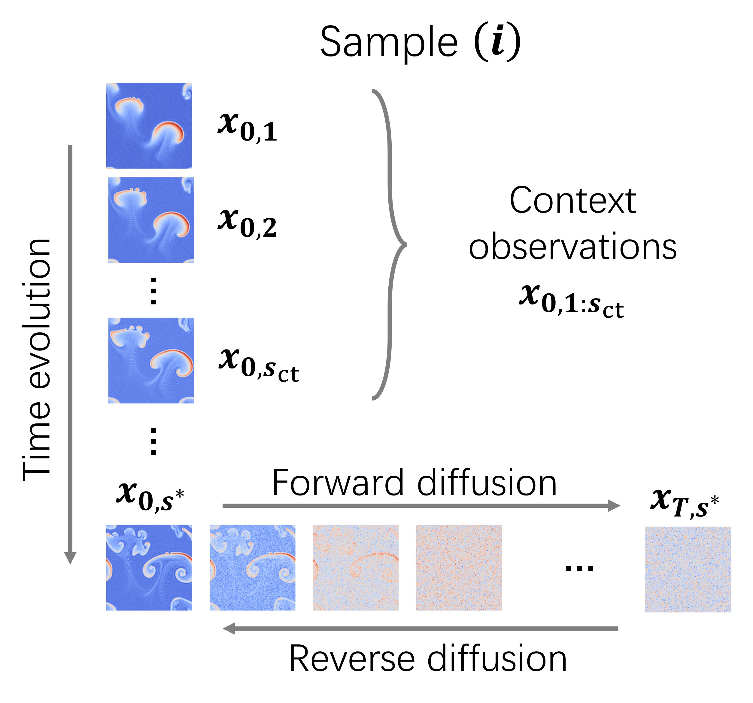
Denoising Diffusion Implicit Models (DDIMs) use a series of Gaussian noise with increasing variance to corrupt the data, then train DeNNs to gradually reconstruct clean data from corrupted ones. The DDIM consists of multiple steps (Ho et al., 2020), each one of which corresponds to a specific level of variance in the Gaussian noise. For clarity, we use to denote the step- diffusion of the state vector observed at time . It is important to note that signifies the diffusion step, whereas indicates the actual time within the dynamic system. Fig. 1 provides a pictorial depiction of this process, illustrating both the diffusion mechanism and the temporal evolution of data.
In DDIM, the forward diffusion process is given as,
| (1) |
where are i.i.d. Gaussian noise vectors and is a predefined constant that determines the noise variances. Similar to Ho et al. (2020), we introduce notation and .
In the continuous limit, the forward diffusion process (1) reduces to a stochastic differential equation (SDE) (Song & Ermon, 2019),
| (2) |
where is the standard Brownian motion or Weiner process. With a slight abuse of notation, the subscript denotes a continuous variable in (2) and a discrete variable in (1). In literature, (2) is often called a variance-preserving SDE (Song & Ermon, 2019).
In the task of future physics state prediction, historic observations are often available to practitioners. We use to denote the number of context (already observed) observations, and as a shorthand notation for the concatenated observed vector (see Time evolution in Fig. 1). Mathematically, the task can be formulated as predicting/sampling the state vector at a time of interest from the predictive distribution , where . The target distribution is a conditional distribution of future state vector given the observed state vectors .
It is important to note that for predictions at multiple future time points, or multiple values of , practitioners can efficiently apply the DDM framework by simply stacking these state vectors and sampling from the the distribution of stacked vectors. Hence, for simplicity and without any loss of generality, we use to signify the state vector at any given target time . Typically in autoregressive tasks, is set to .
To generate high-quality samples, DDMs exploit an existing dataset to learn the target conditional distribution, where the superscript is the observation index. Different denotes different collected evolution trajectories of state vectors. is the total number of trajectories in the training set.
We briefly describe the training objective of DDIM. By iteratively applying (1), one can show that has the same distribution as where is a vector whose elements are i.i.d. standard Gaussians. DDIM leverages such fact to train an iterative DeNN that predicts the noise from the corrupted sample . More specifically, the training objective of DDIM is,
| (3) |
In (3.1), the diffusion and denoising only happen at the target time . The objective is to minimize the difference between the noise added to the sample and the noise predicted by the denoising network. It is worth noting that theoretically, the denoising objective (3.1) is related to the score function in statistics: roughly speaking, if the sample size goes to infinity and (3.1) is exactly minimized, the optimal becomes (Song & Ermon, 2019),
| (4) |
where is the p.d.f. of the random vector , and the score function is the gradient of the logarithm of the p.d.f.
In the inference stage, DDIM (Song et al., 2020) generates high-quality samples from the approximated score functions. More precisely, DDIM samples from the standard normal distribution, then applies the denoising network to iteratively denoise :
| (5) |
for from to . The coefficient will converge to when is small. We obtain eventually.
From the perspective of SDEs, if the denoising network is properly trained as in (3.1), the sampling rule (5) is a discretized version of the reverse process ODE (2),
| (6) |
Under the dynamics specified by (6), the random vector will follow the desired predictive distribution if properly initialized. Such connection justifies (5) theoretically (Song et al., 2020).
3.2 Inexpensive physics-conditioned diffusion
As discussed, the training objective (3.1) and sampling scheme (5) (or the continuous version (6)) only focus on the statistical patterns in the data and can overlook the physics mechanisms, especially when the size of the training dataset is not extremely large. Physics simulations can help alleviate the issue. We assume that simulations can make predictions about the future evolution of the system. The output at time is . We further assume here that the physics simulations are inexpensive, allowing simulation predictions to be obtained for each sample in the training and sampling stages with low latency.
With the physics simulator, we can build an augmented training dataset by combining the training data and inexpensive simulation data at target time , . The augmented dataset enables us to train a conditional diffusion network that takes not only the initial frames but also the simulation prediction as its contextual input.
The training objective of the inexpensive physics-conditioned diffusion model thus becomes
| (7) |
Similar to DDIM, we use Monte Carlo approximation to minimize the objective. The pseudocode is presented in Algorithm 2.
Intuitively, the physics context can bring additional physics knowledge to the model, thus augmenting the authenticity of the prediction. The denoising network is then trained to absorb such physics knowledge. Such intuition is corroborated by our theoretical analysis in Theorem 4.1 (see Section 4).
Accordingly, the iterative sampling rule becomes,
| (8) |
for from to , starting from .
The sampling rule (3.2) is analogous to that in (5). The only difference is that we augment the input to the DeNN with the predictions from the physics simulations. We also provide a pseudocode of the sampling rule as the choice of Algorithm 3. Our experiments show that the augmented information can significantly improve the sampling performance.
3.3 Expensive physics-conditioned diffusion
Clearly, the approach above is simple since simulations are cheap, but what if we have simulations that are expensive? Often, practitioners can obtain physics predictions from more expensive but potentially more accurate physics models. We denote the results from an expensive simulator at time as . Then, an augmented dataset of trajectories and simulations is . However, due to high computation costs or latency, we assume that may only be available for a subset of . Thus, we cannot directly feed into the DeNN. This section employs a different strategy to handle the case where is available. Here, we leverage conditional DDMs to guide the diffusion process by both inexpensive and expensive simulators, namely, . Notably, our method exploits the sparsely available , decoupled from the training procedure in Section 3.2, ensuring that the unavailability of does not affect the training of the denoising network .
We motivate our derivation from the reverse diffusion ODE,
| (9) |
One can see that the conditional score function replaces its counterpart in (6) and plays the central role in the reverse diffusion process. Therefore, it suffices to derive an estimate of the conditional score function.
From the Bayes’s rule, we know for any ,
The first term can be approximated by the denoising network trained by Algorithm 2. We use to denote an estimate of the second term,
| (10) |
In literature, there are multiple ways to construct estimates for . When the conditional probability is known, we introduce a conceptually simple and computationally tractable procedure inspired by (Chung et al., 2023). The pseudocode is presented in Algorithm 1.
In Algorithm 1, step 2 uses the Tweedie’s formula (Chung et al., 2023) to produce a point estimate of the sample given a noisy sample . It essentially removes the noise from the noisy sample with the noise estimated by the DeNN . Then, step 3 and 4 use the (scaled) gradient over the clean sample to approximate . Such a procedure is easy to implement and works well in practice. We will defer detailed derivations to supplementary materials.
It is the practitioner’s discretion to choose the instantiation of in Algorithm 1. In principle, the conditional probability model should reflect how the expensive simulation is related to the observations . We will demonstrate two choices of conditional probability models in the numerical experiments about fumes (5.1) and thermal processes (6.2). In section 3.4, we also present some guidelines for designing the conditional model.
Combining Algorithm 1 with the DDIM discretization of (3.3), a discrete update rule for sampling/inference is,
| (Term 1) | ||||
| (Term 2) | ||||
| (Term 3) |
for from to . In (LABEL:eqn:expensivediffusionsample), (Term 1) corresponds to the component in (3.3), which is essential in the variance-preserving SDE. (Term 2) approximates the score function that drives the sample to high-probability regions predicted by the inexpensive physics simulation . The coefficients are consistent with those in DDIM. Furthermore, (Term 3) represents the conditioning of the expensive physics simulation that furnishes additional guidance to . (Term 3) is the major difference between (LABEL:eqn:expensivediffusionsample) and (3.2). The collective effects of three forces encourage the sample to enter regions where statistical patterns and physics knowledge are congruent.
By initializing from multiple independent samples from the standard normal distribution and iteratively applying (LABEL:eqn:expensivediffusionsample), one can obtain multiple instances of . The sample variances estimated from these instances provide a straightforward characterization for uncertainty quantification.
To summarize, the pseudocodes of the training and sampling algorithms are presented in Algorithm 2 and Algorithm 3.
3.4 Insights for designing the conditional probability
Leveraging domain-specific knowledge is crucial for determining the exact form of the conditional probability model. In literature, numerous successful examples of such models exist (Jacobsen et al., 2023; Song et al., 2021b).
In scenarios where different physics simulations are independent, it is reasonable to simplify the conditional probability as . Our studies demonstrate that this probability can be effectively represented by energy-based models: , where denotes a differentiable energy function and the partition function is neglected as after taking the logarithm, the partition function contributes only a constant term, which becomes zero if we take gradient on . This energy function attains lower values for consistent pairs of simulation and sample and higher values for inconsistent pairs. For instance, if is a coarse-grained prediction for , one could define as . serves as a temperature parameter that modulates the strength of the conditional probability. This model framework promotes consistency between the sample and the corresponding expensive physical simulation. We will explore two applications of the energy-based approach in Sections 5 and 6.
4 Theoretical Analysis
Now, we provide theoretical guarantees for the sampling algorithms in the continuous regime. Remember that the raison d’etre for Algorithm 3 is to obtain samples from and . A natural performance metric for the sampler is thus the distance between the ground truth and sampling distribution.
In this section, we use to denote the distribution of samples generated by Algorithm 3 with choice 1, and to denote the sample distributions from Algorithm 3 with choice 2, where we omit the dependence on , and for brevity. Then a well-behaving algorithm should satisfy and . Similar to (Kwon et al., 2022), we use the Wasserstain distance to quantify the difference between the sampling and ground truth distributions. The Wasserstein distance (Santambrogio, 2015) between two p.d.f. and is denoted as .
Intuitively, the differences between the two distributions result from two sources. The first is the inaccurate denoising network: if cannot learn the score function to high precisions, the sampling distribution can be inaccurate. Mathematically, we define the expected -error between the denoising network prediction and the ground truth score as,
| (12) |
The second source of error originates from inaccurate functions: if does not accurately represent the gradient of the log conditional probability, the sampling algorithm can also be problematic.
| (13) |
The following theorem provides an upper bound on the Wasserstein distance between the sampling and the ground truth distribution.
Theorem 4.1.
Under regularity conditions, if we use Algorithm 3 with choice 1 to sample , in the continuous limit, the sample distribution satisfies,
| (14) |
Similarly, if we use Algorithm 3 with choice 2 to sample , in the continuous limit, the sampling distribution would satisfy,
| (15) |
It is worth noting that in practice, the forward diffusion processes are often designed carefully such that and are extremely close to standard normal distributions (Ho et al., 2020). As such, their Wasserstein distance is often insignificant, and the right-hand side of (4.1) and (4.1) are dominated by and .
There are a few implications from Theorem 4.1. First, (4.1) indicates that if we use choice 1 from Algorithm 3, the sampling distribution error is determined by the prediction error of the denoising network . This is consistent with our intuition that a more accurate denoising network will lead to higher-quality samples. Second, (4.1) suggests that the sampling error for choice 2 is related to the estimation error in both denoising network and the gradient of the log conditional probability model . Accurate and estimates would bring the distribution close to the ground truth .
5 Fluid system
We first investigate the numerical performance of the proposed MPDM on a fluid system. The dynamics of viscous fluids are described by Navier-Stokes equations, which are nonlinear partial differential equations. In practice, Navier-Stokes equations are often solved by computational fluid dynamics (CFD) programs. Numerous CFD programs have been developed in recent decades, and many of them rely on finite difference methods that solve fluid fields on the grids (Anderson & Wendt, 1995). Like many physics simulators, finite difference CFD methods face tradeoffs between grid resolution and simulation fidelity, which renders MPDM a useful tool to integrate the predictions from CFD simulations with different resolutions and leverage the combined knowledge to make predictions.
5.1 Experiment setup
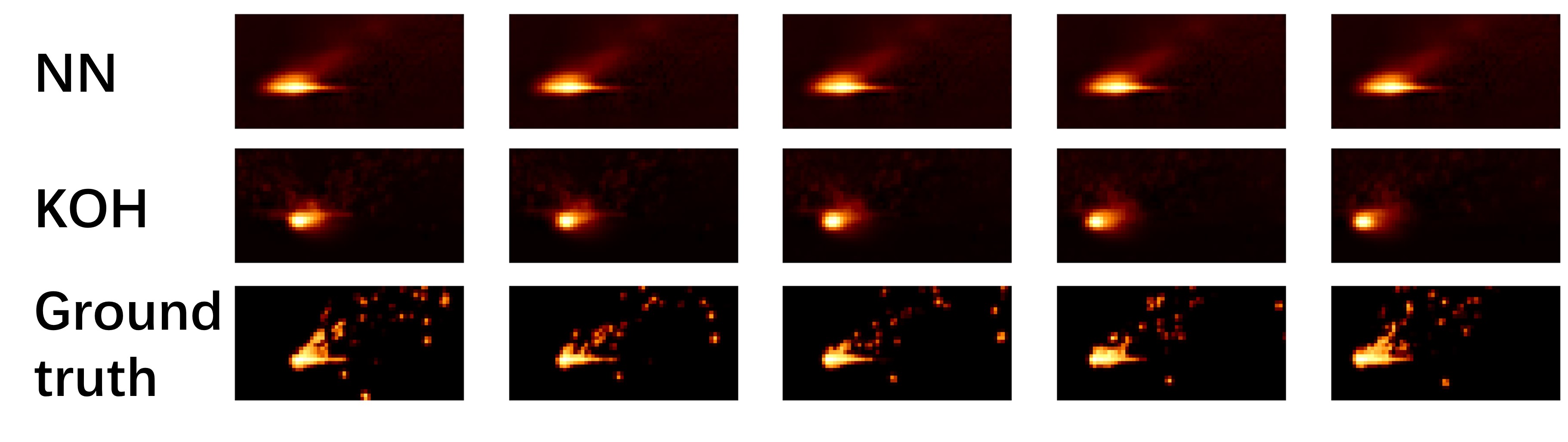
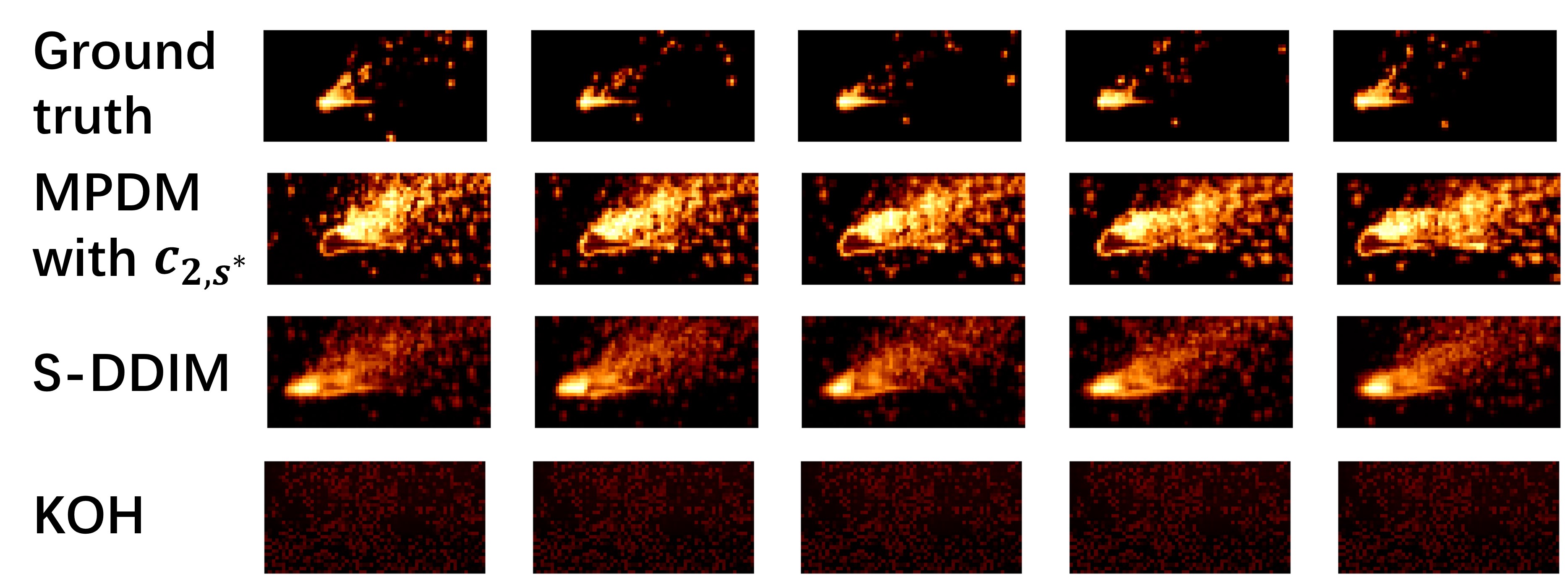
In the numerical study, we analyze the movement of 2D fumes driven by buoyancy and gravity, with the goal of predicting buoyancy fields. We use Boussinesq approximation (Spiegel & Veronis, 1960) to analyze the evolution of the fume system. The ground truth data are generated by running multiple simulations of the fumes with existing high-performance CFD simulators (Mohanan et al., 2019b, a) on fine-grained grids. More specifically, we randomly initialize the buoyancy and vorticity at time and run the simulator from to . We use the buoyancy field at time steps as the context vectors, and predict the target state at . Results of simulations from different random initializations are accumulated and then randomly separated into 90% training set and 10% test set. We train the DeNN on the training set. On the test set, we try to predict with the information , , and possible . The buoyancy at for four samples from the test set is plotted in the last column of Fig. 2.
To apply MPDM, inexpensive physics predictions and expensive physics predictions are needed. We generate these predictions using the same Navier-Stokes-Boussinesq simulator but on coarser grids. More specifically, for each simulation, we run the fluid simulator from the same initialization as the ground truth but with a grid resolution of . The buoyancy and vorticity fields at are the inexpensive physics prediction . Similarly, we run the fluid simulator with a grid resolution of and use the buoyancy as .
Four samples of are plotted in the first column of Fig. 2. One can observe that the inexpensive simulation can capture the low-frequency patterns of the ground truth while details of fume swirls are blurred. This disparity demonstrates the inherent simulation bias.
In this study, we choose the conditional probability model as,
| (16) |
where is an average pooling operation (He et al., 2016) for the patch size of by . More precisely, it divides the buoyancy field into patches of size , then calculates the average buoyancy in each patch. Similarly, is a pooling operation. The model (5.1) encourages the low-frequency information of the simulated buoyancy and predicted buoyancy to be matched. is a coefficient that measures the confidence of the result from the simulated buoyancy. We simply set it to be throughout our experiments. is a normalization constant that will become zero after differentiation. Additionally, we find removing the coefficient in (Term 3) of (LABEL:eqn:expensivediffusionsample) and directly using in the sampling update is more numerically stable. Therefore, we implement this modified version of the sampling update.
5.2 Benchmarks and visual results
With access to physics simulations, we can implement MPDM to predict the ground-truth buoyancy. We use a U-Net (Ronneberger et al., 2015) implemented in (Wang, 2024) as the DeNN. The U-Net structure comprises eight 2D convolutional layers connected via skip connections. The diffusion step input first undergoes transformations through a sequence of sinusoidal functions with varying frequencies, followed by a nonlinear network to output temporal embeddings. These embeddings are then integrated into the intermediate layers of the U-Net through multiplication and addition operations. We use Adam to optimize the U-Net in Algorithm 2.
For comparisons, we also implement benchmark algorithms popular in the literature.
-
•
KOH (Kennedy & O’Hagan, 2000): The Bayesian calibration algorithm (KOH) uses a GP to model the residuals between the physics simulation output and the ground truth. We implement KOH to predict the difference between the ground truth buoyancy and the buoyancy from simulation using a batch-independent multi-output GP model provided by GPytorch (Gardner et al., 2018).
- •
-
•
Standard diffusion (S-DDIM): We implement the method described in Section 3.1 to sample target state vectors without the information from physics simulations.
The predictions of KOH, NN, the S-DDIM in Section 3.1, MPDM with inexpensive physics described in Section 3.2, and MPDM with expensive physics described in Section 3.3 are plotted in Fig. 2.
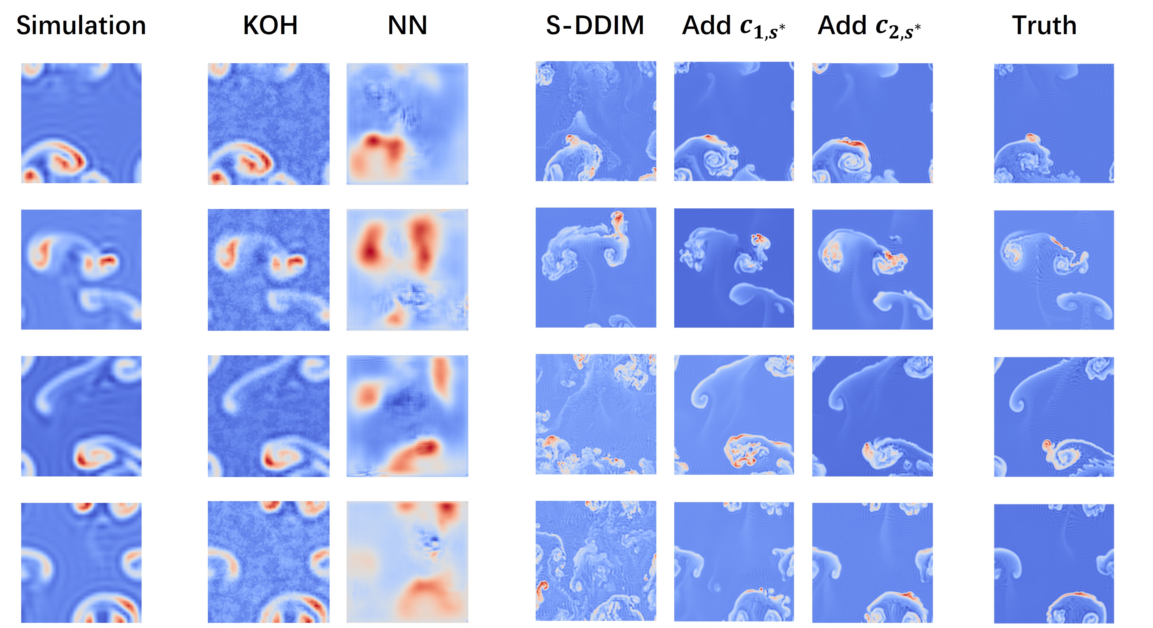
From Fig. 2, we can clearly see that S-DDIM predictions exhibit sharp and vivid details on the small-scale swirling structures of the fume. However, locations of large-scale swirl patterns are not accurate. This indicates that the DeNN learns the localized buoyancy patterns effectively but struggles to understand the long-range physical knowledge. The limitation is addressed when we use inexpensive physics prediction as an additional input to the denoising network. Conditioned on the inexpensive physics prediction, samples from MPDM align more closely with the ground truth in terms of large-scale structures. The results imply that the physics knowledge is integrated in MPDM, which reaps benefits from the simulation while mitigating its bias. Furthermore, when is available and used in choice 2 of Algorithm 3, the fidelity of the buoyancy prediction further improves, indicating that the more refined physics simulations can boost the quality of prediction.
On the contrary, the KOH model does not add meaningful information to the physics simulation, probably because the GP is known to have expressiveness limitations in the high-dimension regime (Wang et al., 2020). As our prediction is a dimensional vector, predicting it using a Gaussian process is uneasy. The NN approach does not give accurate predictions either. This is understandable as NN completely relies on the training set to learn the physical evolution of the fume system. Such a purely statistical approach may not produce decent performance when the training set is not extremely large.
5.3 Numerical performance
For numerical comparisons, we also evaluate the quality of the prediction on four standard evaluation metrics: mean squared error (MSE), peak signal-to-noise ratio (PSNR), structural similarity index (SSIM), and learned perceptual image patch similarity (LPIPS) (Zhang et al., 2018). In general, a lower MSE, a higher PSNR, a higher SSIM, and a lower LPIPS indicate a better sample quality. Amongst these metrics, MSE and PSNR measure the low-level pixel-wise difference between the sample and the ground truth, while SSIM is more aligned with human perception of the images. LPIPS leverages a deep neural network (VGG) to capture high-level visual similarities. The mean and standard deviation on the test set are reported in Table 1. In each column, the best result is highlighted in bold, while the second-best result is emphasized with an underline.
| MSE (0.01) | PSNR | SSIM | LPIPS | |
| KOH | 19.0(0.3) | 99.86(0.01) | 0.582(0.004) | |
| NN | 1.8(0.1) | 18.2(0.2) | 99.83(0.01) | 0.634(0.006) |
| S-DDIM | 5.6(0.2) | 13.2(0.2) | 99.48(0.02) | 0.555(0.003) |
| With | 3.6(0.1) | 15.4(0.2) | 99.69(0.01) | 0.406(0.006) |
| With | 1.6(0.1) | 19.2(0.3) | 99.89(0.01) | 0.345(0.006) |
Results presented in Table 1 corroborate visual observations depicted in Fig. 2. S-DDIM is capable of generating samples that visually resemble the ground truth, as evidenced by its low LPIPS scores when compared with those from KOH and NN methods. However, the model’s high MSE and low PSNR indicate a poorer alignment with the ground truth at pixel levels.
With inexpensive physics predictions , MPDM enhances the sample quality as the LPIPS decreases. Furthermore, there are noticeable improvements in MSE, PSNR, and SSIM relative to the standard DDMs. Incorporation of the expensive physics simulation into the reverse diffusion process (LABEL:eqn:expensivediffusionsample) leads to even greater improvements. The LPIPS scores decrease further, and the MSE, PSNR, and SSIM reach the highest values compared to all other evaluated algorithms. These improvements substantiate the benefits of utilizing multiple simulations in Algorithm 3.
In comparison, the benchmark KOH and NN incur high LPIPS, corroborating our observations that these samples do not show consistent visual patterns as the ground truth. The comparisons highlight the advantages of the proposed MPDM in producing high-quality results.
6 Thermal process in 3D printing
We further apply MPDM on a real-life process of laser-based metal additive manufacturing (LBMAM). LBMAM uses a laser beam to heat and melt metal powders deposited on the printbed to print 3D objects layer by layer (Grasso & Colosimo, 2019; Shi et al., 2024). To monitor the manufacturing process, a thermal camera is installed to capture in-situ temperature distribution on the printing surface. The thermography provides rich information for characterizing the process and potentially identifying defects (Scime & Beuth, 2019; Guo et al., 2023). From a statistics perspective, we aim to predict a future frame of the thermal video, given some observed frames and the information about the movement of the laser that can be recovered from the G-code of the printer.
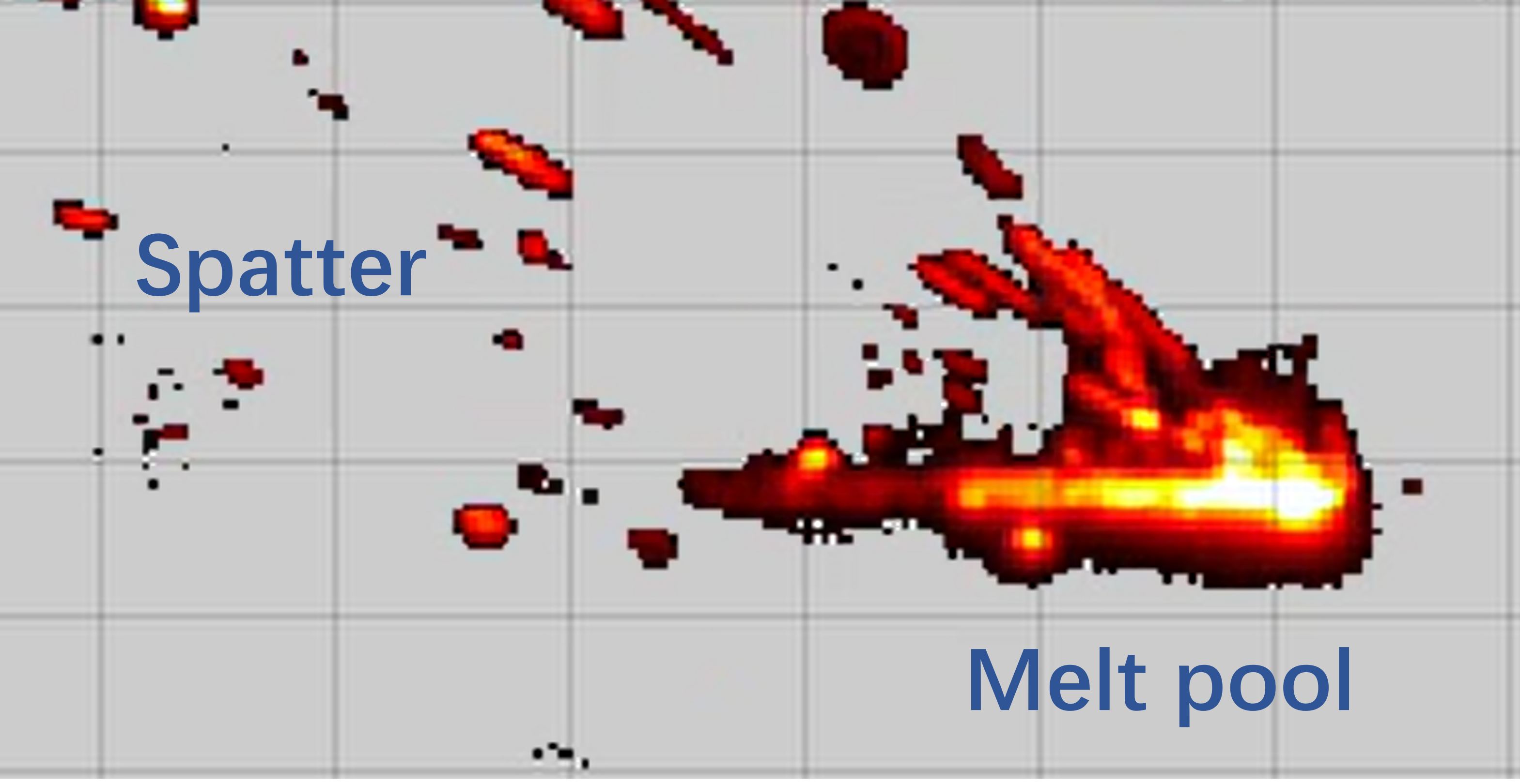
A typical thermal frame from an LBMAM process is plotted in Fig. 3, where the underlying physics in the thermal process can roughly be divided into the melt pool’s heat dissipation and the spatters’ movement (Guo et al., 2022; Grasso et al., 2018). We use two ad-hoc physics models to simulate them. The melt pool is the connected high-temperature region around the laser beam. Its dynamics are described by a 2D heat equation, which has a simple closed-form solution in the ideal case. The solution is easy to calculate; hence we model it as . The spatters are more volatile and irregular. We use a flow model to describe its movement. Compared to the heat pool PDE, the flow model incurs a higher computational cost. Thus, we model the flow velocity field as . We will describe the details of the two models in this section. It is worth noting that both physics models are oversimplified and thus biased, yet our goal is to fuse data with inaccurate physics simulations to get superior predictions.
For notational consistency, we use to denote the pixeled vectorized frame in a thermal video. If the frame has resolution , then is a vector . With a slight abuse of notation, we use to denote the continuous spatial coordinate on the 2D plane. We sometimes use the abbreviated notation . Furthermore, we use to denote a time-varying temperature field on 2D: . We use subscripts and to represent the temperature field of the melt pool and spatters. A thermal video frame naturally corresponds to the temperature at by grid locations.
6.1 Dynamics of the melt pool
The melt pool often displays comet-like shapes, which is a result of heat dissipation and laser movement. In this section, we will construct a computationally amenable model to simulate the morphology and dynamics of the melt pool.
6.1.1 Heat equation
We use to denote the melt pool temperature at point at time .
A natural way to model the physics of is the 2D heat equation,
| (17) |
where the term represents heat dissipation. is the thermal diffusivity matrix,
| (18) |
Term represents the loss of heat from the printing surface into the air, and represents the energy injected by the laser beam at .
6.1.2 Solution in the ideal case
Exactly solving (17) is uneasy as the diffusivity can be anisotropic and temperature-dependent and location-dependent, and the same for the parameter . The boundary condition can also be complicated. Conventional physics simulators are often based on discrete element analysis (Lee & Zhang, 2015) or SPH (Russell et al., 2018).
To obtain a conceptually simple and computationally tractable physical solution, we can make a few simplifying assumptions. We assume and are temperature-independent constants. The initial condition is . And the 2D plane extends to infinity.
Then the solution to (17) is given by,
| (19) |
where is the Green’s function,
| (20) |
and denotes the system parameters.
In (6.1.2), is given by the Gcode of 3D printers. Therefore, the evolution of temperature is controlled by only parameters , , , and . We calibrate these four parameters from data using nonlinear least squares. More specifically, on a dataset of observed temperature on grid , we optimize parameter to fit the observations by empirical error minimization , where denotes the temperature evaluated at grid points. Since the empirical loss is differentiable, the minimization is implemented by Adam. Though is fixed in theoretical derivation (6.1.2), we still calibrate it from data to adapt to the different scalings of and .
6.2 Dynamics of the spatters
The interaction between high-energy laser beams and metal powders generates high-temperature particles that scatter from the metal surface. These particles can also be captured by the thermal camera. However, the 2D heat dissipation PDE can hardly describe the movement of particles. As a result, an alternative physics model is needed.
As the high-temperature particles are heated by the energy from the laser, it is natural to model them to be created at the center of the meltpool. After generation, these particles will move toward the edge of the receptive field of the thermal camera. The optical flow model (Horn & Schunck, 1981) provides a suitable characterization for such an emanating movement pattern.
More specifically, we define a velocity field denoting the velocity of the particle at position and time . The velocity field is the expensive physics simulation . We use to denote the velocity along the -axis and to denote the velocity at the -axis. For a small time interval , the temperature of the scattering particles should remain approximately constant. As a result, should satisfy,
This equation is widely employed in the literature of optical flows (Horn & Schunck, 1981).
In practice, the optical flow may not be perfectly accurate because of the modeling, measurement, optimization, and statistical errors. We thus use the following probability model to characterize the inaccuracy,
| (21) |
where are i.i.d. standard Gaussians noise. The parameter represents our prior belief about the model accuracy: a larger implies a higher confidence in the flow model. Therefore, given the optical flow , the conditional probability is,
Since we predict the temperature only on discrete pixels rather than the continuous 2D plane, the discrete counterpart of the equation above is,
| (22) |
where plays the role of the expensive simulation .
In (6.2), denotes the warping operator, which employs a semi-Lagrangian method to infer from and . A more detailed definition of will be provided in the supplementary material. denotes the projection into the spatter region, , defined as follows,
Intuitively, applies a mask that selects the spatter temperature distribution from the entire temperature field. In our implementation, we define as the complement of the melt pool region, which we estimate from the PDE solution (6.1.2).
6.3 Case study
We use a subset of the 2018 AM Benchmark Test Series from NIST (Heigel et al., 2020) as a testbed of the LBMAM thermal video prediction model. The dataset is collected in an alloy LBMAM process of a bridge structure manufactured in layers. An infrared camera with a frame rate of frames per second is installed for in-situ thermography.
We select the thermal videos captured when printing the first layers and slice them into video clips, each of which contains frames. The clips where the laser beam moves outside the camera receptive field are discarded since they are not informative. Each clip is a trajectory of the thermal process of LBMAM. On each clip, we use the beginning frames as the context frames and predict the last frames. We also perform an 80%-20% train-test splitting and present the results on the test set.
As discussed, the solution (6.1.2) at is modeled as inexpensive physics predictions , which is plotted as the first row of Fig. 4. PDE solutions precisely identify the location of the melt pool. However, compared to the real thermal frames, the PDE solutions are excessively smooth, failing to capture the complex geometries of the melt pool and the spatters.
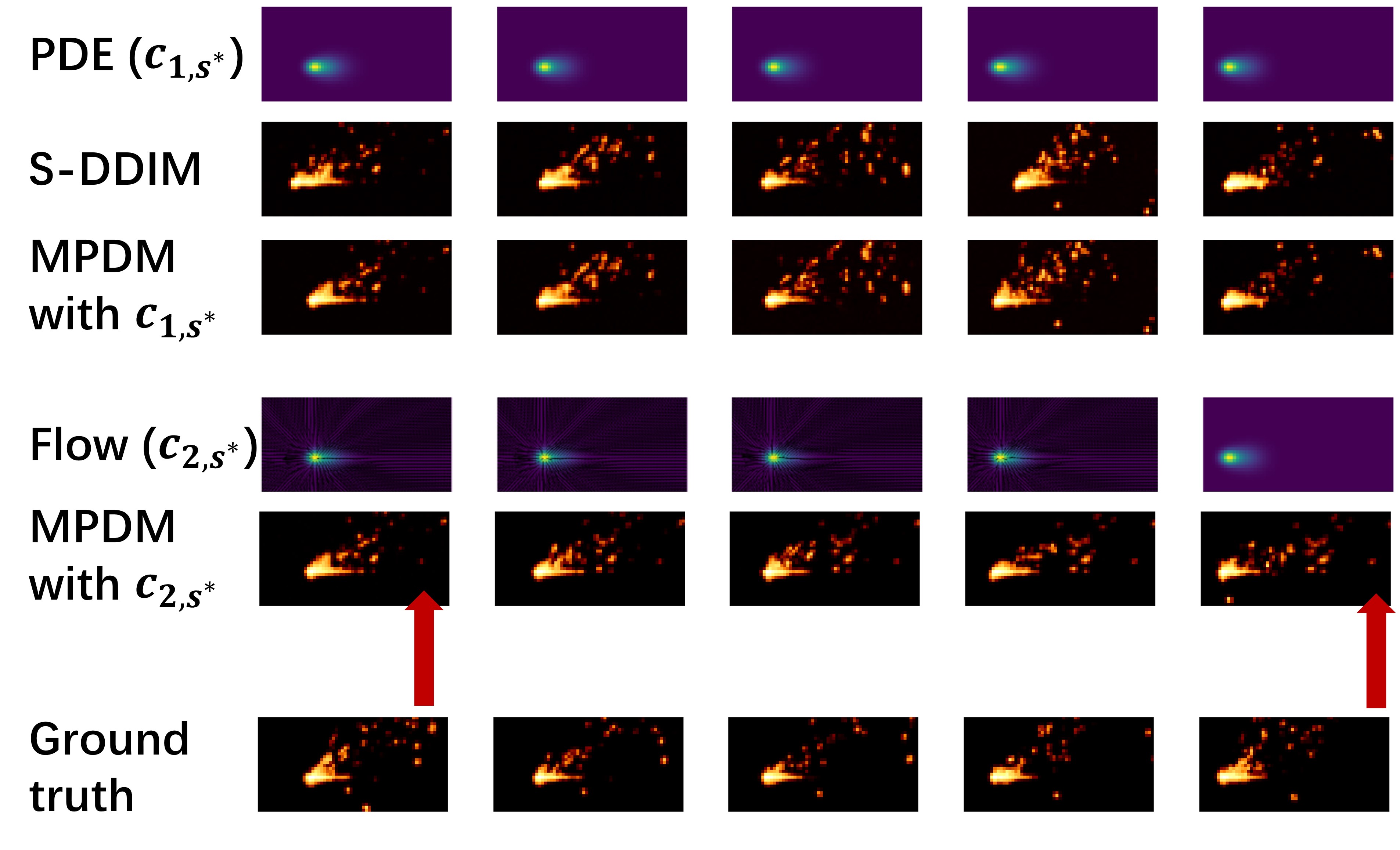
Conversely, S-DDIM generates more realistic and intricate temperature distributions. As illustrated in the second row of Fig. 4, the irregular contours of the melt pool and the spatial arrangement of spatters bear a closer resemblance to those observed in ground truth data. Nevertheless, the positioning of the melt pool, as predicted by S-DDIM, is inaccurate, indicating deficiencies in the model’s capability to track the dynamics of melt pool movement.
MPDM integrates the strengths of both PDE-based solutions and the diffusion model. Using the available , we train the DeNN by Algorithm 2, as elaborated in Section 3.2. The results are shown in the third row of Fig. 4. These results vividly illustrate how DDMs can enhance the fine geometric details of the melt pool on top of PDE solutions. Our approach improves the accuracy of predicting the locations of the melt pool while simultaneously preserving the detailed realism of the temperature field.
Though the single-frame prediction of inexpensive physics-informed diffusion demonstrates verisimilitude, the spatter patterns across frames are not consistent in Fig. 4. Therefore, we add flow information to model the evolution of spatters as described in Section 6.2. The estimated flow fields on the test frames are plotted as small black arrows in the fourth row of Fig. 4. Then, we use the flow field as the expensive physics simulation and sample thermal frames with Algorithm 3 with choice 2. Results are plotted in the fifth row of Fig. 4. As highlighted by the red arrows, the flow information makes spatter movement patterns more consistent.
For comparisons, we also implement KOH and NN as benchmarks. Detailed implementation procedures conform to the specifications described in Section 5.2. The resulting predictions are illustrated in Fig. 5.
In Fig. 5, results from NN and KOH are visually distinct from the ground truth. Specifically, the temperature distributions produced by NN appear over-dispersed. Similarly, the predictions by KOH lack meaningful spatter patterns observed in the ground truth data. When compared to the results depicted in Fig. 4, it is evident that both PINN and KOH yield predictions with geometric patterns that are less consistent with those of the ground truth.
6.4 Numerical evaluation
To thoroughly assess the performance of different approaches, we also calculate the PSNR, SSIM, and LPIPS between the predictions and the ground truth. The detailed settings are similar to Section 5.3. Additionally, to evaluate the cross-frame consistency, we leverage the flow model to evaluate the consistency score between frames. The consistency score is defined as
where is the flow prediction at time . The consistency score measures how well the movement of spatters in samples complies with the flow model. Apparently, a lower consistency score signifies a higher level of cross-frame realism. The mean and standard deviation of different metrics evaluated on the test set are reported in Table 2.
| PSNR | SSIM | LPIPS | CS | |
|---|---|---|---|---|
| KOH | 25.1(0.4) | 99.976(0.003) | 0.27(0.01) | 0.22(0.03) |
| NN | 24.0(0.2) | 99.960(0.002) | 0.24(0.01) | 0.064(0.008) |
| S-DDIM | 21.3(0.2) | 99.924(0.004) | 0.166(0.002) | 1.43(0.03) |
| With | 24.3(0.2) | 99.977(0.006) | 0.140(0.002) | 1.41(0.02) |
| With | 24.2(0.2) | 99.976(0.007) | 0.136(0.005) | 0.064(0.005) |
Table 2 shows that the PDE solution significantly improves the sample quality for the diffusion model, as suggested by increases in PSNR and SSIM and a decrease in LPIPS. Such results are consistent with the visual observations in Fig. 4. Additionally, the use of flow fields further improves the sample quality and drastically decreases the consistency score, which validates the observation in Fig. 4 that the spatter patterns move more consistently.
For benchmark methods, though KOH attains a high PSNR value, its LPIPS score is high, suggesting that while KOH’s predictions are accurate at a pixel level, they do not align well with human perceptual judgments. This observation is supported by Fig. 5, which shows that the modifications introduced by the KOH model to the PDE solutions are minor and barely perceptible. Therefore, similar to PDE solutions, KOH predictions lack spatters. Such results differ significantly from the ground truths in geometric patterns, thus incurring high LPIPS values. Results for the NN model suggest that its sample quality is not satisfactory either compared to MPDM with choice 2.
6.5 Uncertainty quantification
The probabilistic nature of MPDM provides a straightforward approach to uncertainty quantification. In this case study, we independently sample samples according to standard DDMs and Algorithm 3 with choice 2, and calculate pixel-wise standard deviations of the samples. The results are shown in Fig. 6.
Among benchmark algorithms, only KOH is capable of uncertainty quantification. We thus also plot the standard deviation of the learned GP in KOH in Fig. 6.
Fig. 6 illustrates that the predictive variance of MPDM is high in spatter regions and low within the melt pool area. This pattern aligns with expectations, as spatters display irregular and dynamic behaviors in thermal videos, whereas the melt pool movement is more predictable. In contrast, S-DDIM without physics simulation information predicts high variance in the meltpool area, suggesting that the model is unsure about the location of the meltpool. The comparison highlights the advantage of Algorithm (3) in predictive variance reduction. The predictive uncertainty derived from KOH does not provide meaningful insights. The contrast further illustrates MPDM’s ability to accurately characterize the distribution of the evolution of physical systems.
7 Conclusion and future research directions
This paper introduces MPDM, a generative framework based on multi-fidelity physics simulations and diffusion processes. MPDM is proved theoretically well-grounded and exhibits decent performance on the buoyancy and thermal video prediction tasks. We envision that the flexibility of MPDM would engender broader applications in manufacturing and beyond.
In the case studies presented in this paper, the parameters within the physics models are assumed known a priori or are calibrated (by nonlinear least square fitting) prior to deploying the MPDM model. Consequently, an intriguing avenue for future research would be to integrate parameter calibration directly within the probabilistic diffusion model framework. Additionally, the implications of MPDM on experimental design also merit future explorations.
8 Supplementary Material
References
- Anderson & Wendt (1995) Anderson, J. D. and Wendt, J. Computational fluid dynamics, volume 206. Springer, 1995.
- Benjamin et al. (2019) Benjamin, S. G., Brown, J. M., Brunet, G., Lynch, P., Saito, K., and Schlatter, T. W. 100 years of progress in forecasting and nwp applications. Meteorological Monographs, 59:13–1, 2019.
- Chen et al. (2023) Chen, W., Wu, J., Xie, P., Wu, H., Li, J., Xia, X., Xiao, X., and Lin, L. Control-a-video: Controllable text-to-video generation with diffusion models. arXiv preprint arXiv:2305.13840, 2023.
- Chung et al. (2023) Chung, H., Kim, J., Mccann, M. T., Klasky, M. L., and Ye, J. C. Diffusion posterior sampling for general noisy inverse problems. In The Eleventh International Conference on Learning Representations, 2023. URL https://openreview.net/forum?id=OnD9zGAGT0k.
- Chung et al. (2024) Chung, H., Lee, S., and Ye, J. C. Decomposed diffusion sampler for accelerating large-scale inverse problems. In The Twelfth International Conference on Learning Representations, 2024. URL https://openreview.net/forum?id=DsEhqQtfAG.
- Cuomo et al. (2022) Cuomo, S., Di Cola, V. S., Giampaolo, F., Rozza, G., Raissi, M., and Piccialli, F. Scientific machine learning through physics–informed neural networks: Where we are and what’s next. Journal of Scientific Computing, 92(3):88, 2022.
- De Bortoli et al. (2022) De Bortoli, V., Mathieu, E., Hutchinson, M., Thornton, J., Teh, Y. W., and Doucet, A. Riemannian score-based generative modelling. Advances in Neural Information Processing Systems, 35:2406–2422, 2022.
- Fishman et al. (2023) Fishman, N., Klarner, L., De Bortoli, V., Mathieu, E., and Hutchinson, M. Diffusion models for constrained domains. arXiv preprint arXiv:2304.05364, 2023.
- Fonseca Guerra et al. (1998) Fonseca Guerra, C., Snijders, J., Te Velde, G. t., and Baerends, E. J. Towards an order-n dft method. Theoretical Chemistry Accounts, 99:391–403, 1998.
- Gardner et al. (2018) Gardner, J., Pleiss, G., Weinberger, K. Q., Bindel, D., and Wilson, A. G. Gpytorch: Blackbox matrix-matrix gaussian process inference with gpu acceleration. Advances in neural information processing systems, 31, 2018.
- Gramacy (2020) Gramacy, R. B. Surrogates: Gaussian process modeling, design, and optimization for the applied sciences. Chapman and Hall/CRC, 2020.
- Grasso & Colosimo (2019) Grasso, M. and Colosimo, B. A statistical learning method for image-based monitoring of the plume signature in laser powder bed fusion. Robotics and Computer-Integrated Manufacturing, 57:103–115, 2019. ISSN 0736-5845. doi: https://doi.org/10.1016/j.rcim.2018.11.007. URL https://www.sciencedirect.com/science/article/pii/S073658451830139X.
- Grasso et al. (2018) Grasso, M., Demir, A., Previtali, B., and Colosimo, B. In situ monitoring of selective laser melting of zinc powder via infrared imaging of the process plume. Robotics and Computer-Integrated Manufacturing, 49:229–239, 2018. ISSN 0736-5845. doi: https://doi.org/10.1016/j.rcim.2017.07.001. URL https://www.sciencedirect.com/science/article/pii/S0736584517300583.
- Guo et al. (2022) Guo, S., Agarwal, M., Cooper, C., Tian, Q., Gao, R. X., Guo, W., and Guo, Y. Machine learning for metal additive manufacturing: Towards a physics-informed data-driven paradigm. Journal of Manufacturing Systems, 62:145–163, 2022. ISSN 0278-6125. doi: https://doi.org/10.1016/j.jmsy.2021.11.003.
- Guo et al. (2023) Guo, S., Guo, W., Bian, L., and Guo, Y. B. A deep-learning-based surrogate model for thermal signature prediction in laser metal deposition. IEEE Transactions on Automation Science and Engineering, 20(1):482–494, 2023. doi: 10.1109/TASE.2022.3158204.
- He et al. (2016) He, K., Zhang, X., Ren, S., and Sun, J. Deep residual learning for image recognition. In Proceedings of the IEEE Conference on Computer Vision and Pattern Recognition (CVPR), June 2016.
- Heigel et al. (2020) Heigel, J. C., Lane, B., Levine, L., Phan, T., and Whiting, J. In situ thermography of the metal bridge structures fabricated for the 2018 additive manufacturing benchmark test series (am-bench 2018). Journal of Research of the National Institute of Standards and Technology, 125, 2020.
- Ho et al. (2020) Ho, J., Jain, A., and Abbeel, P. Denoising diffusion probabilistic models. Advances in neural information processing systems, 33:6840–6851, 2020.
- Ho et al. (2022a) Ho, J., Chan, W., Saharia, C., Whang, J., Gao, R., Gritsenko, A., Kingma, D. P., Poole, B., Norouzi, M., Fleet, D. J., et al. Imagen video: High definition video generation with diffusion models. arXiv preprint arXiv:2210.02303, 2022a.
- Ho et al. (2022b) Ho, J., Salimans, T., Gritsenko, A., Chan, W., Norouzi, M., and Fleet, D. J. Video diffusion models. arXiv:2204.03458, 2022b.
- Horn & Schunck (1981) Horn, B. K. and Schunck, B. G. Determining optical flow. Artificial intelligence, 17(1-3):185–203, 1981.
- Huang et al. (2022) Huang, C.-W., Aghajohari, M., Bose, J., Panangaden, P., and Courville, A. C. Riemannian diffusion models. Advances in Neural Information Processing Systems, 35:2750–2761, 2022.
- Huang et al. (2023) Huang, J., Pang, Y., Liu, Y., and Yan, H. Posterior regularized bayesian neural network incorporating soft and hard knowledge constraints. Knowledge-Based Systems, 259:110043, 2023.
- Iyer (2011) Iyer, G. Kolmogorov forward equation. Lecture notes for Advanced Stochastic Calculus, 2011. URL https://www.math.cmu.edu/~gautam/teaching/2011-12/880-advanced-scalc/pdfs/kolmogorov-forward.pdf.
- Jacobsen et al. (2023) Jacobsen, C., Zhuang, Y., and Duraisamy, K. Cocogen: Physically-consistent and conditioned score-based generative models for forward and inverse problems. arXiv preprint arXiv:2312.10527, 2023.
- Jalal et al. (2021) Jalal, A., Arvinte, M., Daras, G., Price, E., Dimakis, A. G., and Tamir, J. Robust compressed sensing mri with deep generative priors. Advances in Neural Information Processing Systems, 34:14938–14954, 2021.
- Ji et al. (2023) Ji, Y., Mak, S., Soeder, D., Paquet, J., and Bass, S. A. A graphical multi-fidelity gaussian process model, with application to emulation of heavy-ion collisions. Technometrics, pp. 1–15, 2023.
- Jiao et al. (2024) Jiao, R., Huang, W., Lin, P., Han, J., Chen, P., Lu, Y., and Liu, Y. Crystal structure prediction by joint equivariant diffusion. Advances in Neural Information Processing Systems, 36, 2024.
- Karsch (2002) Karsch, F. Lattice qcd at high temperature and density. In Lectures on quark matter, pp. 209–249. Springer, 2002.
- Kennedy & O’Hagan (2000) Kennedy, M. C. and O’Hagan, A. Predicting the output from a complex computer code when fast approximations are available. Biometrika, 87(1):1–13, 2000.
- Kennedy & O’Hagan (2001) Kennedy, M. C. and O’Hagan, A. Bayesian calibration of computer models. Journal of the Royal Statistical Society: Series B (Statistical Methodology), 63(3):425–464, 2001.
- Kollovieh et al. (2024) Kollovieh, M., Ansari, A. F., Bohlke-Schneider, M., Zschiegner, J., Wang, H., and Wang, Y. B. Predict, refine, synthesize: Self-guiding diffusion models for probabilistic time series forecasting. Advances in Neural Information Processing Systems, 36, 2024.
- Kovachki et al. (2023) Kovachki, N., Li, Z., Liu, B., Azizzadenesheli, K., Bhattacharya, K., Stuart, A., and Anandkumar, A. Neural operator: Learning maps between function spaces with applications to pdes. Journal of Machine Learning Research, 24(89):1–97, 2023.
- Kwon et al. (2022) Kwon, D., Fan, Y., and Lee, K. Score-based generative modeling secretly minimizes the wasserstein distance. Advances in Neural Information Processing Systems, 35:20205–20217, 2022.
- Lam et al. (2023) Lam, R., Sanchez-Gonzalez, A., Willson, M., Wirnsberger, P., Fortunato, M., Alet, F., Ravuri, S., Ewalds, T., Eaton-Rosen, Z., Hu, W., et al. Learning skillful medium-range global weather forecasting. Science, 382(6677):1416–1421, 2023.
- Lee & Zhang (2015) Lee, Y. and Zhang, W. Mesoscopic simulation of heat transfer and fluid flow in laser powder bed additive manufacturing. 2015 International Solid Freeform Fabrication Symposium, 2015.
- Lewis et al. (2020) Lewis, P., Perez, E., Piktus, A., Petroni, F., Karpukhin, V., Goyal, N., Küttler, H., Lewis, M., Yih, W.-t., Rocktäschel, T., et al. Retrieval-augmented generation for knowledge-intensive nlp tasks. Advances in Neural Information Processing Systems, 33:9459–9474, 2020.
- Li et al. (2022) Li, Y., Lu, X., Wang, Y., and Dou, D. Generative time series forecasting with diffusion, denoise, and disentanglement. In Koyejo, S., Mohamed, S., Agarwal, A., Belgrave, D., Cho, K., and Oh, A. (eds.), Advances in Neural Information Processing Systems, volume 35, pp. 23009–23022. Curran Associates, Inc., 2022. URL https://proceedings.neurips.cc/paper_files/paper/2022/file/91a85f3fb8f570e6be52b333b5ab017a-Paper-Conference.pdf.
- Li et al. (2020) Li, Z., Kovachki, N., Azizzadenesheli, K., Liu, B., Bhattacharya, K., Stuart, A., and Anandkumar, A. Fourier neural operator for parametric partial differential equations. arXiv preprint arXiv:2010.08895, 2020.
- Liu et al. (2023) Liu, P., Yuan, W., Fu, J., Jiang, Z., Hayashi, H., and Neubig, G. Pre-train, prompt, and predict: A systematic survey of prompting methods in natural language processing. ACM Computing Surveys, 55(9):1–35, 2023.
- Lu et al. (2021) Lu, L., Jin, P., Pang, G., Zhang, Z., and Karniadakis, G. E. Learning nonlinear operators via deeponet based on the universal approximation theorem of operators. Nature machine intelligence, 3(3):218–229, 2021.
- Mak et al. (2018) Mak, S., Sung, C.-L., Wang, X., Yeh, S.-T., Chang, Y.-H., Joseph, V. R., Yang, V., and Wu, C. J. An efficient surrogate model for emulation and physics extraction of large eddy simulations. Journal of the American Statistical Association, 113(524):1443–1456, 2018.
- Midjourney (2024) Midjourney. Midjourney showcase, 2024. URL https://www.midjourney.com/showcase.
- Mohanan et al. (2019a) Mohanan, A. V., Bonamy, C., and Augier, P. FluidFFT: Common API (c and python) for fast fourier transform HPC libraries. Journal of Open Research Software, 7, 2019a. doi: 10.5334/jors.238.
- Mohanan et al. (2019b) Mohanan, A. V., Bonamy, C., Linares, M. C., and Augier, P. FluidSim: Modular, Object-Oriented Python Package for High-Performance CFD Simulations. Journal of Open Research Software, 7, 2019b. doi: 10.5334/jors.239.
- OpenAI (2024) OpenAI. Video generation models as world simulators, 2024. URL https://openai.com/research/video-generation-models-as-world-simulators.
- Raissi et al. (2017) Raissi, M., Perdikaris, P., and Karniadakis, G. E. Physics informed deep learning (part i): Data-driven solutions of nonlinear partial differential equations. arXiv preprint arXiv:1711.10561, 2017.
- Raissi et al. (2019) Raissi, M., Perdikaris, P., and Karniadakis, G. Physics-informed neural networks: A deep learning framework for solving forward and inverse problems involving nonlinear partial differential equations. Journal of Computational Physics, 378:686–707, 2019. ISSN 0021-9991. doi: https://doi.org/10.1016/j.jcp.2018.10.045. URL https://www.sciencedirect.com/science/article/pii/S0021999118307125.
- Ramesh et al. (2022) Ramesh, A., Dhariwal, P., Nichol, A., Chu, C., and Chen, M. Hierarchical text-conditional image generation with clip latents. arXiv preprint arXiv:2204.06125, 1(2):3, 2022.
- Rombach et al. (2022) Rombach, R., Blattmann, A., Lorenz, D., Esser, P., and Ommer, B. High-resolution image synthesis with latent diffusion models. In Proceedings of the IEEE/CVF conference on computer vision and pattern recognition, pp. 10684–10695, 2022.
- Ronneberger et al. (2015) Ronneberger, O., Fischer, P., and Brox, T. U-net: Convolutional networks for biomedical image segmentation. In Medical image computing and computer-assisted intervention–MICCAI 2015: 18th international conference, Munich, Germany, October 5-9, 2015, proceedings, part III 18, pp. 234–241. Springer, 2015.
- Russell et al. (2018) Russell, M., Souto-Iglesias, A., and Zohdi, T. Numerical simulation of laser fusion additive manufacturing processes using the sph method. Computer Methods in Applied Mechanics and Engineering, 341:163–187, 2018.
- Santambrogio (2015) Santambrogio, F. Optimal transport for applied mathematicians. Birkäuser, NY, 55(58-63):94, 2015.
- Scime & Beuth (2019) Scime, L. and Beuth, J. Using machine learning to identify in-situ melt pool signatures indicative of flaw formation in a laser powder bed fusion additive manufacturing process. Additive Manufacturing, 25:151–165, 2019. ISSN 2214-8604. doi: https://doi.org/10.1016/j.addma.2018.11.010.
- Shi et al. (2024) Shi, N., Guo, S., and Al Kontar, R. Personalized feature extraction for manufacturing process signature characterization and anomaly detection. Journal of Manufacturing Systems, 74:435–448, 2024.
- Shu et al. (2023) Shu, D., Li, Z., and Barati Farimani, A. A physics-informed diffusion model for high-fidelity flow field reconstruction. Journal of Computational Physics, 478:111972, 2023. ISSN 0021-9991. doi: https://doi.org/10.1016/j.jcp.2023.111972. URL https://www.sciencedirect.com/science/article/pii/S0021999123000670.
- Song et al. (2020) Song, J., Meng, C., and Ermon, S. Denoising diffusion implicit models. arXiv preprint arXiv:2010.02502, 2020.
- Song & Ermon (2019) Song, Y. and Ermon, S. Generative modeling by estimating gradients of the data distribution. Advances in neural information processing systems, 32, 2019.
- Song et al. (2021a) Song, Y., Durkan, C., Murray, I., and Ermon, S. Maximum likelihood training of score-based diffusion models. Advances in neural information processing systems, 34:1415–1428, 2021a.
- Song et al. (2021b) Song, Y., Shen, L., Xing, L., and Ermon, S. Solving inverse problems in medical imaging with score-based generative models. arXiv preprint arXiv:2111.08005, 2021b.
- Spiegel & Veronis (1960) Spiegel, E. A. and Veronis, G. On the boussinesq approximation for a compressible fluid. Astrophysical Journal, vol. 131, p. 442, 131:442, 1960.
- Spitieris & Steinsland (2023) Spitieris, M. and Steinsland, I. Bayesian calibration of imperfect computer models using physics-informed priors. Journal of Machine Learning Research, 24(108):1–39, 2023.
- Stability AI (2024) Stability AI. Stable diffusion 3, 2024. URL https://stability.ai/stable-image.
- Sun & Wang (2020) Sun, L. and Wang, J.-X. Physics-constrained bayesian neural network for fluid flow reconstruction with sparse and noisy data. Theoretical and Applied Mechanics Letters, 10(3):161–169, 2020.
- Swiler et al. (2020) Swiler, L. P., Gulian, M., Frankel, A. L., Safta, C., and Jakeman, J. D. A survey of constrained gaussian process regression: Approaches and implementation challenges. Journal of Machine Learning for Modeling and Computing, 1(2), 2020.
- Thieme (2018) Thieme, H. R. Mathematics in population biology, volume 1. Princeton University Press, 2018.
- Urain et al. (2023) Urain, J., Funk, N., Peters, J., and Chalvatzaki, G. Se (3)-diffusionfields: Learning smooth cost functions for joint grasp and motion optimization through diffusion. In 2023 IEEE International Conference on Robotics and Automation (ICRA), pp. 5923–5930. IEEE, 2023.
- Wang (2024) Wang, P. denoising-diffusion-pytorch. https://github.com/lucidrains/denoising-diffusion-pytorch/tree/main, 2024.
- Wang et al. (2020) Wang, W., Tuo, R., and Jeff Wu, C. On prediction properties of kriging: Uniform error bounds and robustness. Journal of the American Statistical Association, 115(530):920–930, 2020.
- Wang et al. (2024) Wang, X., Yuan, H., Zhang, S., Chen, D., Wang, J., Zhang, Y., Shen, Y., Zhao, D., and Zhou, J. Videocomposer: Compositional video synthesis with motion controllability. Advances in Neural Information Processing Systems, 36, 2024.
- Williams & Rasmussen (2006) Williams, C. K. and Rasmussen, C. E. Gaussian processes for machine learning, volume 2. MIT press Cambridge, MA, 2006.
- Yang et al. (2023) Yang, L., Zhang, Z., Song, Y., Hong, S., Xu, R., Zhao, Y., Zhang, W., Cui, B., and Yang, M.-H. Diffusion models: A comprehensive survey of methods and applications. ACM Computing Surveys, 56(4):1–39, 2023.
- Yang et al. (2020) Yang, W., Lorch, L., Graule, M., Lakkaraju, H., and Doshi-Velez, F. Incorporating interpretable output constraints in bayesian neural networks. Advances in Neural Information Processing Systems, 33:12721–12731, 2020.
- Zhang et al. (2018) Zhang, R., Isola, P., Efros, A. A., Shechtman, E., and Wang, O. The unreasonable effectiveness of deep features as a perceptual metric. In Proceedings of the IEEE conference on computer vision and pattern recognition, pp. 586–595, 2018.
- Zhang et al. (2020) Zhang, R., Liu, Y., and Sun, H. Physics-guided convolutional neural network (phycnn) for data-driven seismic response modeling. Engineering Structures, 215:110704, 2020.
- Zhu et al. (2019) Zhu, Y., Zabaras, N., Koutsourelakis, P.-S., and Perdikaris, P. Physics-constrained deep learning for high-dimensional surrogate modeling and uncertainty quantification without labeled data. Journal of Computational Physics, 394:56–81, 2019.
Appendix A Derivations in Algorithm 1
In this section, we will discuss the intuitions for Algorithm 1 in the main paper. The goal is to derive an estimate for . The derivation is inspired by Chung et al. (2023).
We first use the Bayes law to rewrite as,
where is a constant independent of .
As the integral can be difficult to calculate analytically, we resort to approximations. There are a few feasible approximations, among which we will use the most conceptually simple and computationally tractable one. Since we have trained a denoising network , we can approximate by Tweedie’s formula (Chung et al., 2023),
where is the Dirichlet-delta function and is defined as,
| (23) |
With the approximation, we can calculate the gradient as,
We can use the Leibniz rule to further expand the gradient as,
The exact calculation of requires taking the gradient of a high dimensional variable through a neural network, which can be memory-consuming. To save memory, we thus employ another approximation by ignoring the gradient contributed by the denoising network, . Combing these two approximations, we have,
Appendix B Derivations of the solution to the heat equation
The Green’s function solves the following equation
| (24) |
where is the Dirichelet delta function.
We can use the Fourier transform to solve the equation. Due to translational invariance, the Fourier series of is given by,
| (25) |
When , the solution to (26) is simply,
Therefore, the original Green’s function is
It consists of a exponential decaying component , a Gaussian component , and a constant .
Appendix C Optical flow and wrapping
As discussed, represents the vecterized temperature at time evaluated on the grids. We also use to denote the velocity on the same grids. The wrapping operator uses and to predict , which is the temperature at time defined on the grids.
We implement the wrapping operator via a semi-Lagrangian approach. An illustration of the numerical advection is shown in Fig. 7.
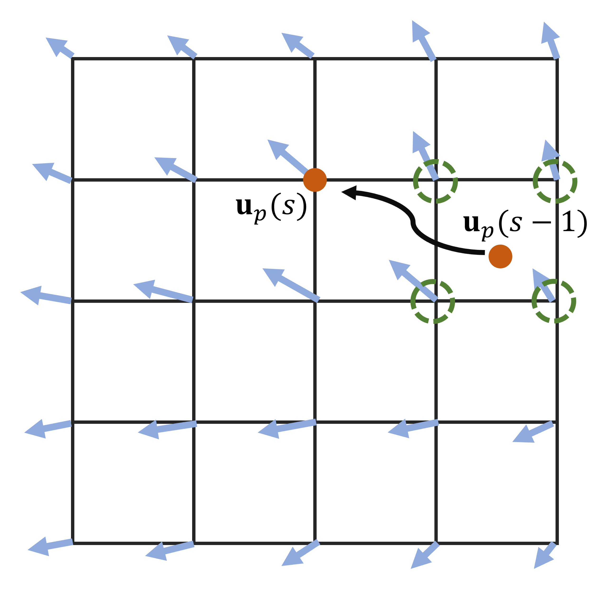
More specifically, for any grid location , the algorithm estimates its location at time as is , then predict as . However, as shown in Fig. 7, the orange dot representing may not sit exactly on the grid point. Thus, is not readily known. To resolve the issue, we use bilinear interpolation to interpolate the velocity based on the grid velocity on the closest grids, which are shown as the green circles in Fig. 7.
We provide a pseudo-code for the wrapping operator as,
In Algorithm 4, interpolate is the standard bilinear interpolation from the closest grid points. The entire operation is differentiable.
Appendix D Proof for Theorem 4.1
In this section, we present the proof for Theorem 4.1 in the main paper. In literature, the Wasserstein distance is defined as,
| (27) |
where is the set of all joint distributions of whose marginal distributions are and .
We will begin by introducing a useful inequality that provides an upper bound of the Wasserstein distance between the distributions given by two PDEs. Similar versions of this inequality have already been derived in literature (Kwon et al., 2022).
Lemma D.1.
Consider two p.d.f. and in that satisfy the following PDEs respectively,
| (PDE1) | |||
| (PDE2) |
where are drift terms that satisfy the regularity conditions in (Kwon et al., 2022). If additionally, there exists a finite function , such that for each , , then, the Wasserstain distance satisfies
We outline the proof of Lemma D.1 for completeness.
Proof.
The proof follows (Kwon et al., 2022).
Corollary 5.25 in (Santambrogio, 2015) provides an important relation that describes the evolution of the Wasserstain distance between and ,
| (28) |
under refularity conditions, where is the optimal transport map from to .
The right hand side of (28) can be expanded as,
For the first term, Cauchy-Schwartz inequality indicates,
The second term can be lower bounded by the assumption of Lipschitz continuity,
Combining them, we know that
This implies,
| (29) |
By integrating both sides for from to , we complete the proof. ∎
With Lemma D.1, we can prove Theorem 4.1 in the main paper. We assume the regularity conditions in (Kwon et al., 2022) are satisfied. Additionally, we assume that there are constants , such that for all possible tuple , the following holds,
| (30) |
Proof.
We first consider the sampling algorithm with choice . In the continuous regime, the forward diffusion process is characterized by
The forward Kolmogorov equation (Iyer, 2011) shows that the p.d.f. follows a PDE,
As discussed, the sampling algorithm with choice 1 reduces to an ODE in the continuous regime,
| (31) |
and initalizes from the standard normal distribution . By forward Kolmogorov equation, the p.d.f. of , , satisfy,
It is straightforward to set , , and apply Lemma D.1. We first provide an upper bound of the Lipshitz constant from the assumptions. For any , we have,
where we used the inequality and .
Therefore, Lemma D.1 implies,
where we used Cauchy-Schwartz inequality in the last inequality and is defined as,
Then, we proceed to analyze the sampling algorithm with choice 2. The ideal reverse process conditioned on and is given by,
| (32) |
The corresponding Kolmogorov equation is given by,
Similarly, the continuous form of the approximate reverse process employed by choice 2 of the sampling algorithm is
| (33) |
Its corresponding Kolmogorov equation is,
Similarly, if we set and , we can calculate . As a result, Lemma D.1 indicates
From the inequality , we have,
Combining them, we know
where is defined as,
This completes our proof. ∎