Multi-messenger Detection Rates and distributions of Binary Neutron Star Mergers and Their Cosmological Implications

The observations of GW170817/GRB 170817A suggest it has a Gaussian-shaped jet profile (Zhang & Mészáros, 2002; Troja et al., 2018; Alexander et al., 2018; Mooley et al., 2018; Lazzati et al., 2018; Ghirlanda et al., 2019)

for $\iota\leq\iota_{w}$, where $E_{0}$ is the on-axis equivalent isotropic energy, $\iota_{c}$ is the characteristic angle of the core, $\iota_{w}$ is the truncating angle of the jet. Troja et al. (2018) give the constraints on the jet with $\iota_{c}=0.057^{+0.025}_{-0.023}$, $\log_{10}E_{0}=52.73^{+1.3}_{-0.75}$, $\iota_{w}=0.62^{+0.65}_{-0.37}$. We assume all BNS mergers in our simulation has a relativistic jet with this profile. In order to convent this energy profile to the luminosity profile, we assume the burst duration $T_{90}\sim 2$ s (Abbott et al., 2017d) and the spectrum is flat with time during the burst, where $T_{90}$ is defined as the duration of the period which 90% of the burst’s energy is emitted. So, the $\gamma$-ray flux of each BNS mergers can be written as

where $\eta_{\gamma}$ is the radiative efficiency and we adopt it as 0.1 for the bolometric energy flux in the 1 - 10⁴ keV band. We assume the spectrum for all BNS-associated-GRBs follow the Band function

Here $N(E)$ is in units of photons cm^-2 s^-1 keV^-1 and $E_{p}$ corresponds to the peak energy in the $\nu F_{\nu}$ spectra. We adopt the photon indices $\alpha$ and $\beta$ as, -1 and -2.3 (Preece et al., 2000) below and above the peak energy $E_{p}$ respectively. However, the bolometric isotropic luminosity $L$ and the peak energy for GRB 170817A do not follow the $E_{p}-L$ relation for short $\gamma$-ray bursts (Zhang & Wang, 2018) and long $\gamma$-ray bursts (Yonetoku et al., 2004), which can be written as

There is a profile proposed by Ioka & Nakamura (2019) that the peak energy $E_{p}$ changes with $\iota$ with following relationship

within the Gaussian structure jet framework, where $E_{p,0}$ is the peak energy that satisfies the Yonetoku relation. This profile makes the GRB170817a observations consistent with previous GRB observation.

With the peak energy and the Band function, we can get the effective sensitivity limit for various $\gamma$-ray detectors. Here we adopt the same setting as Song et al. (2019), the sensitivity for Fermi-GBM is adopted as $\sim 2\times 10^{-7}\ \mathrm{erg}\ \mathrm{s}^{-1}\ \mathrm{cm}^{-2}$ in 50 keV to 300 keV (Meegan et al., 2009), the sensitivity for GECAM is adopted as $\sim 1\times 10^{-7}\ \mathrm{erg}\ \mathrm{s}^{-1}\ \mathrm{cm}^{-2}$ in 50 keV to 300 keV (Zhang et al., 2018), the sensitivity for Swift-BAT and SVOM-ECLAIRS is adopted as $\sim 1.2\times 10^{-8}\ \mathrm{erg}\ \mathrm{s}^{-1}\ \mathrm{cm}^{-2}$ in 15 keV to 150 keV (Gehrels et al., 2004; Götz et al., 2014), and the sensitivity for Einstein Probe (EP) is adopted as $\sim 3\times 10^{-9}\ \mathrm{erg}\ \mathrm{s}^{-1}\ \mathrm{cm}^{-2}$ in 0.5 keV to 4 keV (Yuan et al., 2018). Another important factor affecting the detection ability of the $\gamma$-ray detector is the size of its field of view. For Fermi-GBM, its field of view (FOV) covers about 3/4 of the whole sky and for GECAM, the field of view is about 4$\pi$. For other three detectors, their fields of view are much smaller. The factors are $\sim$ 1/9 for Swift-BAT, $\sim$ 1/5 for SVOM-ECLAIRS (Chu et al., 2016) and $\sim$ 1/11 for EP compared with the whole sky. Note that, these $\gamma$-ray detectors might have no overlapped observational time with future 3G GW detector networks. However, we expect the similar or more powerful detectors in 3G era. So, for simplification, throughout this paper we only consider these $\gamma$-ray detectors for illustration.

The measurements of GRBs’ redshift relies on the identification of their host galaxies and further optical observations. And the afterglow usually plays a crucial role in the host galaxy identification. In this paper, we use the standard afterglow models (Sari et al., 1998) to estimate the afterglows on $R$ band. The spectra and light curve are determined by the inclination angle $\iota$, the half-opening angle $\theta_{j}$, the total kinetic energy $E_{j}=(1-\cos\theta_{j})E_{0}$, the number density of the interstellar medium (ISM) $n_{0}$, the magnetic field energy fraction $\epsilon_{B}$, the accelerated electron energy fraction $\epsilon_{e}$, the power-law index of shock-accelerated $p$, the luminosity distance $d_{L}$ and the time after merger in unit of days $t_{j}$.

With adopting the convention notion $Q=10^{x}Q_{,x}$, for a adiabatic jet, the Lorentz factor is given by (Sari et al., 1998)

For an on-axis observer, a phenomenon named jet break is expected when $\gamma$ drops below $\theta_{j}$ and the jet’s material begin to spread sideways (Sari et al., 1998; Mészáros & Rees, 1999). At the jet break time, there will be a break in the afterglow’s light curve. From Eq. (12), the jet break time $t_{j}$ is given by

At the jet-break time, there are two cases for flux density, $F_{\nu,j}$, the slow-cooling case ($\nu_{m}<\nu<\nu_{c}$) and the fasting cooling cases ($\nu_{c}<\nu$), where $\nu_{m}$ is the typical synchrotron frequency of the accelerated electrons with the minimum Lorentz and $\nu_{c}$ is the cooling frequency. In the slow-cooling case, $F_{\nu,j}\propto\nu^{-(p-1)/2}$, where we adopt $p=2.2$ in this paper (the same as Nakar et al. (2002) and Zou et al. (2007)). While in the fast-cooling case, $F_{\nu,j}\propto\nu^{-p/2}$ (Sari et al., 1998).

For an on-axis observer, the light curve is divided into two power-law segments by the jet break time (Sari et al., 1998). We denote the temporal decay index of the flux density $F_{\nu,0}(t)$ in the time as $\alpha_{1}$ and $\alpha_{2}$, which represent the time before and after $t_{j}$, respectively. The index $\alpha_{1}$ is $-(2-3p)/4$ in the fast cooling case and $-3(1-p)/4$ in the slow cooling case. When $t>t_{j}$, the on-axis observer can only observe $\sim\theta_{j}^{2}\gamma^{2}$ of the flux density in the isotropic fireball case. Since $\gamma(t)\propto t^{-3/8}$, we have $\alpha_{2}=\alpha_{1}+3/4$.

For a point source moving at angle $\iota$, the observed flux is (Granot et al., 2002)

where $d_{A}$ is the angular distance, $L^{\prime}_{\nu^{\prime}}$ and $\nu^{\prime}$ are the jet comoving frame spectral luminosity and frequency. For an off-axis observer $(t,\nu)$ at the angle $\iota$ and an on-axis observer $(t_{0},\nu_{0})$ at the angle 0, there are $t_{0}/t\approx\nu/\nu_{0}=(1-\beta)/(1-\beta\cos\iota)\equiv a$, where $\beta=\sqrt{1-1/\gamma^{2}}$. And we obtain

Here we consider both fast and slow cooling cases, which are $\nu_{c}<\nu$ and $\nu_{m}<\nu<\nu_{c}$, respectively.

Since we find $z=3$ has exceeded the detection limit of the GRB detectors in the simulations, we set it as the upper redshift limit and sampled $10^{7}$ BNS mergers. However, this upper limit is too high for the 2G interferometers that the simulation became very inefficient with them. The upper detection limit with LHVIK A+ is about $z\sim 0.2$, so for the 2G interferometers, we resample them with $z\in(0,0.3]$.

There are $\sim 3.4\times 10^{5}$ BNS samples detected by ET and $5.1\times 10^{6}$ detected by CE. For 2G GW detector networks LHV, LHVIK, LHV A+ and LHVIK A+, the numbers are $2.7\times 10^{4}$, $5.7\times 10^{4}$, $1.6\times 10^{5}$ and $3.3\times 10^{5}$, respectively, with samples’ $z\in(0,0.3]$. The observation ability of A+ type network will improve several times even with less detectors. About 10-12% BNS mergers’ GW signal observed by 2G GW detector networks could be triggered by $\gamma$-ray detector. For 3G detectors, the fractions are much lower because more events have high redshift.

We convert these numbers into rates per year, after multiplying the total rate of BNS mergers. Integrating Eq. (1), in $z\in(0,0.3]$, the total rate is 1159-11736 yr^-1 and in $z\in(0-3]$, the total rate is $6.9\times 10^{4}-7.0\times 10^{5}$ yr^-1. Due to the limited observation area of the $\gamma$-ray detectors, not all GRB events whose flux reaches the threshold count be observed. So the multi-messenger observation rates require a discount, FOV/$\Omega_{0}$, where $\Omega_{0}$ is the solid angle of whole sky. Table 1 lists the observation rates per year with this discount. For LHV, the rate is 0.042-0.425 per year with Swift-BAT and 0.072-0.731 per year with SVOM-ECLAIRS. For GECAM and Fermi-GBM, the rates are a few times larger due to their much larger observation areas. The result of EP is slightly worse than Swift-BAT due to its smaller observation area, although it has better sensitivity. After adding two LIGO-type detectors, the rates of LHVIK are about twice as large as LHV. The future upgrade of aLIGO, A+ would increase these numbers by about five times. For 3G interferometers ET, their will be about $100\sim 800$ multi-messenger observation rate with different $\gamma$-ray detectors if we adopt 810 Gpc^-3yr^-1 as the local merger rate. The rates are much larger even only with one single interferometer. For another 3G interferometer CE, the rates are a few times larger compared with ET, since it has a further observation range. It is worth noting that we assume the GW and GRB detections are independent. However, in the real situation, with a triggered GRB, one can search weaker GW signals. So the numbers in Table 1 might be slightly smaller compared to the actual situation.

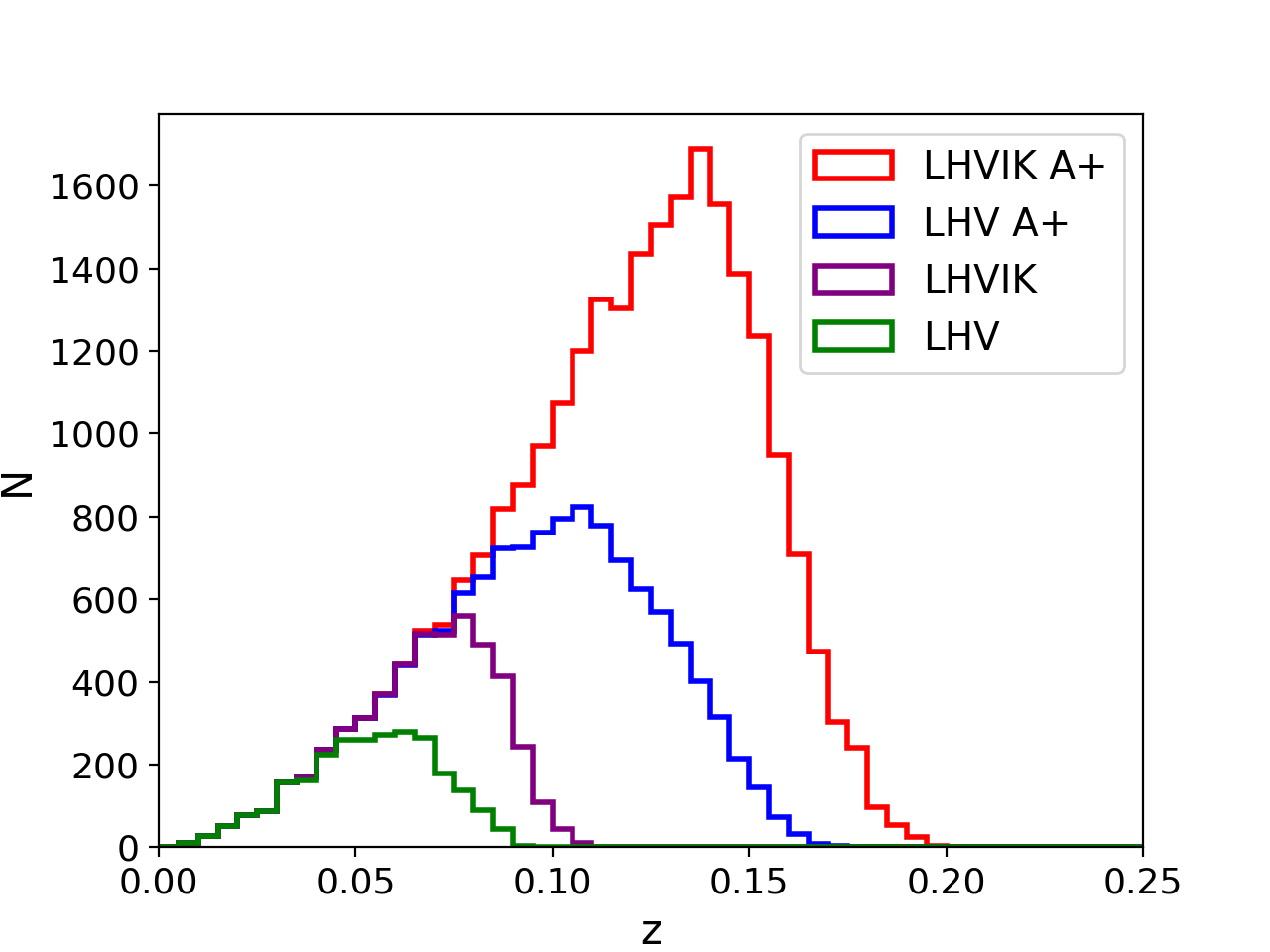
We select the BNS samples that can be triggered by both GW interferometers and $\gamma$-ray detectors. We choose the result of GECAM as a representative and show their redshift distribution in Fig. 1. The redshift limits of LHV and LHVIK are around $z\sim 0.1$ and the the detection limit of LHVIK A+ can reach $\sim 0.2$ due to more sensitive detection capabilities. For 3G interferometers ET and CE, the redshift limits are $z\sim 1.0$ and $z\sim 2.5$, respectively.

As an important method for measuring redshift information, we also calculate the magnitude of GRB afterglows with the method mentioned in Subsection 4.2. We adopt $n_{0}=1\ \mathrm{cm}^{-3}$, $p=2.2$, $\epsilon_{e}=0.1$, $\epsilon_{B}=0.01$, $p=2.2$, where they are the same as Nakar et al. (2002) and Zou et al. (2007). For the half opening angle, we consider three cases, $\theta_{j}=5^{\circ},\ 10^{\circ},\ 15^{\circ}$. For off-axis samples, we calculate the afterglows’ maximum $R$ band magnitude $M_{R}$ with different opening angles respectively. However, for on-axis GRB samples, their afterglows power-low decay with time and we cannot get their maximum $M_{R}$ from their light curve, as showed in Fig. 2, so we denote the $R$ band flux in the jet break time as $M_{R}$ in this case, as a comparison with the off-axis samples.

Using the case of GECAM and $\theta_{j}=10^{\circ}$ as an example, we show the distributions of standard sirens’ redshift, inclination angle and the flux of afterglows in Fig. 3. From these figures, we can intuitively see the $\iota$ limit of multi-messenger observation. In very low redshift, there is a BNS sample with $\iota\sim 22^{\circ}$. This sample’s inclination angle and redshift are very similar with GW170817. For samples with $z=1$, the $\iota$ limit becomes to about $15^{\circ}$. Zhao et al. (2011) and Sathyaprakash et al. (2010) have roughly estimated the distribution of GW sources on the order of magnitude, which is about 1000 per year with inclination angle $\iota<20^{\circ}$. These predictions are based on the $\sim$ several $\times 10^{5}$ BNS rate per year within the horizon of ET, and $\sim 10^{-3}$ of them will have GRBs toward us. These estimates meet well with our result. We use the improved measurement of BNS merger rate from GW observations and give stronger constraints on the multi-messenger event rates. In the next subsection, we will use their methods, combined with our results of simulations, to show the potential of determination of dark energy by the 3G GW interferometers ET and CE. The design specification of LSST for $5\sigma$ depths for point sources in the $r$ band is $\sim 24.7$ (Ivezić et al., 2019), which correspond to point sources and fiducial zenith observations. Due to the small inclination angles, all standard sirens have $M_{R}$ brighter it. For 2.5-meter Wide Field Survey Telescope (WFST), the sigle-visit depth with a 30 s exposure time is $r\sim 22.8$. A small fraction of samples in the case of SVOM fainter than $r\sim 22.8$. If we consider a 300 s exposure time, the sigle-visit depth of WFST will reach $r\sim 24.1$ and all samples have $M_{R}$ brighter than it. In other two choices of $\theta_{j}$, their afterglows all reach the design depth of LSST and WFST. Therefore, we have assume all multi-messenger BNS events in our simulation have a detectable afterglow and we can measure their redshift from their afterglows.

In Fig. 4, we set the number density of ISM as $n_{0}=0.1\ \mathrm{cm}^{-3}$ and $n_{0}=0.01\ \mathrm{cm}^{-3}$ as a comparison, respectively. GRB surrounded by thinner ISM usually has a weaker afterglow. In the case of $n_{0}=0.01\ \mathrm{cm}^{-3}$, a small fraction of afterglows are fainter than the design depth of LSST and WFST. In that case, the measurement of GRBs’ redshift seems difficult and further discussion is needed.

In the last two decades, the accelerated expansion of the universe has been confirmed by a series of observations (Kowalski et al., 2008; Hicken et al., 2009; Komatsu et al., 2009; Eisenstein et al., 2005; Percival et al., 2007, 2010; Schrabback et al., 2010; Kilbinger et al., 2009). Various models of dark energy have been proposed to explain it (see Copeland et al. (2006) for a review). In order to understand the physical properties of dark energy, it is important to measure its equation of state (EOS). In Sathyaprakash et al. (2010) and Zhao et al. (2011), the new method of measuring the dark energy EOS using GW standard sirens was proposed. Zhao & Wen (2018) compared the results of GW detector networks with 1000 face-on BNS sources, with baryon acoustic oscillations (BAO) method, and Type Ia supernovas (SNIa) method, and found that by the 3G GW detector networks, the constraints of dark energy parameters are similar with the SNIa and BAO methods. In this subsection, we will discuss these constraints with a quantitatively distributed BNS sample.

Similar to Zhao et al. (2011), we adopt a phenomenological form for EOS parameter $w$ as a function of redshift (Chevallier & Polarski, 2001)

where $p_{\mathrm{de}}$ is the pressure of dark energy and $\rho_{\mathrm{de}}$ is the energy density. The parameter $w_{0}$ represent the present EOS and $w_{a}$ represent the evolution with redshift. In the $\Lambda$CDM model, the relation of $d_{L}-z$, is determined by $(H_{0},\ \Omega_{m},\ \Omega_{k},\ w_{0},\ w_{a})$ together (Weinberg, 2008). So if the $d_{L}-z$ relation can be measured from a series of multi-messenger observations, the set of these 5 parameters would have chance to be constrain. However, due to the strong degeneracy between the background parameters $(H_{0},\ \Omega_{m},\ \Omega_{k})$ and the dark energy parameter $(w_{0},\ w_{a})$, the constraints of full parameters set seems unrealistic (Zhao et al., 2011). The same problem also happens in other methods for dark energy detection (e.g., SNIa and BAO methods) (Albrecht et al., 2006; Zhao et al., 2011). A general way to break this degeneracy is to combine the result with the CMB data, which are sensitive to the background parameters $(H_{0},\ \Omega_{m},\ \Omega_{k})$, and provide the necessary complement to the GW data. It has also been discovered in (Zhao et al., 2011) that taking the Planck CMB observation as a prior is nearly equivalent to treating the parameters $(H_{0},\ \Omega_{m},\ \Omega_{k})$ as known in the data analysis. Thus, similar to Zhao & Wen (2018), Zhao et al. (2018) and Yan et al. (2020), in this article we use the GW data to constrain the dark energy parameters $(w_{0},\ w_{a})$ only.

To estimate the errors of $(w_{0},\ w_{a})$, we consider a Fisher matrix $F_{ij}$ for a collection of $N$ BNS mergers that follows our sample distribution, which is given by (Zhao et al., 2011)

where $i$ and $j$ run from 1 to 2, denoting the free parameter $w_{0}$ and $w_{a}$, and $\hat{\gamma}$ represents the angle $(\alpha,\ \delta,\ \iota,\ \psi)$. The distance error $\delta d_{L}/d_{L}$ have two components: the instrument error $\Delta d_{L}/d_{L}$, and the error caused by the effects of weak lensing. We denote this error as $\tilde{\Delta}d_{L}/d_{L}$ and assume it satisfies $\tilde{\Delta}d_{L}/d_{L}=0.05z$ (Sathyaprakash et al., 2010; Zhao et al., 2011; Zhao & Wen, 2018; Wang & Wang, 2019). So the total distance error could be estimated from $\delta d_{L}/d_{L}=\sqrt{\left(\Delta d_{L}/d_{L}\right)^{2}+\left(\tilde{\Delta}d_{L}/d_{L}\right)^{2}}$. Similar to Gupta et al. (2019) and Zhao & Santos (2019), in order to evaluate $\Delta d_{L}$ for each event, we assume the parameters $(\alpha,\ \delta,\ \iota)$ are constrained well by $\gamma$-ray observation and consider a Fisher matrix of six parameters, $(\psi,\ M,\ \eta,\ t_{c},\ \phi_{c},\ \log d_{L})$. This scenario is possible as we have already have seen in the case of GW170817. The sky position of GW170817 was constrained by finding the host galaxy NGC 4993 (LSC et al., 2017) whereas the inclination angle was constrained from the X-ray and ultraviolet observations (Evans et al., 2017). In Fig. 5 we use the case of GECAM as a representative case and show the distribution of samples instrument errors with two single 3G GW detectors, ET and CE. There is an obvious cutoff around $\Delta\log\ d_{L}\sim 0.08$, since the instrument errors have a strong correlation with SNR and we choose SNR$=12$ as the threshold.

The uncertainties of cosmological parameters are given by $\Delta w_{0}=(F^{-1})_{11}$ and $\Delta w_{a}=(F^{-1})_{22}$. If the statistical errors are dominant, the uncertainties of $w_{0}$ and $w_{a}$ are proportional to $1/\sqrt{N}$. In Table 2, we list the 68.3% (1-$\sigma$) uncertainties of $w_{0}$ and $w_{a}$ marginalized over other parameter with one year’s multi-messenger observation. Also, to estimate the goodness of parameter constraints, we list the figure of merit (FoM) (Albrecht et al., 2006) in Table 2, which is written as

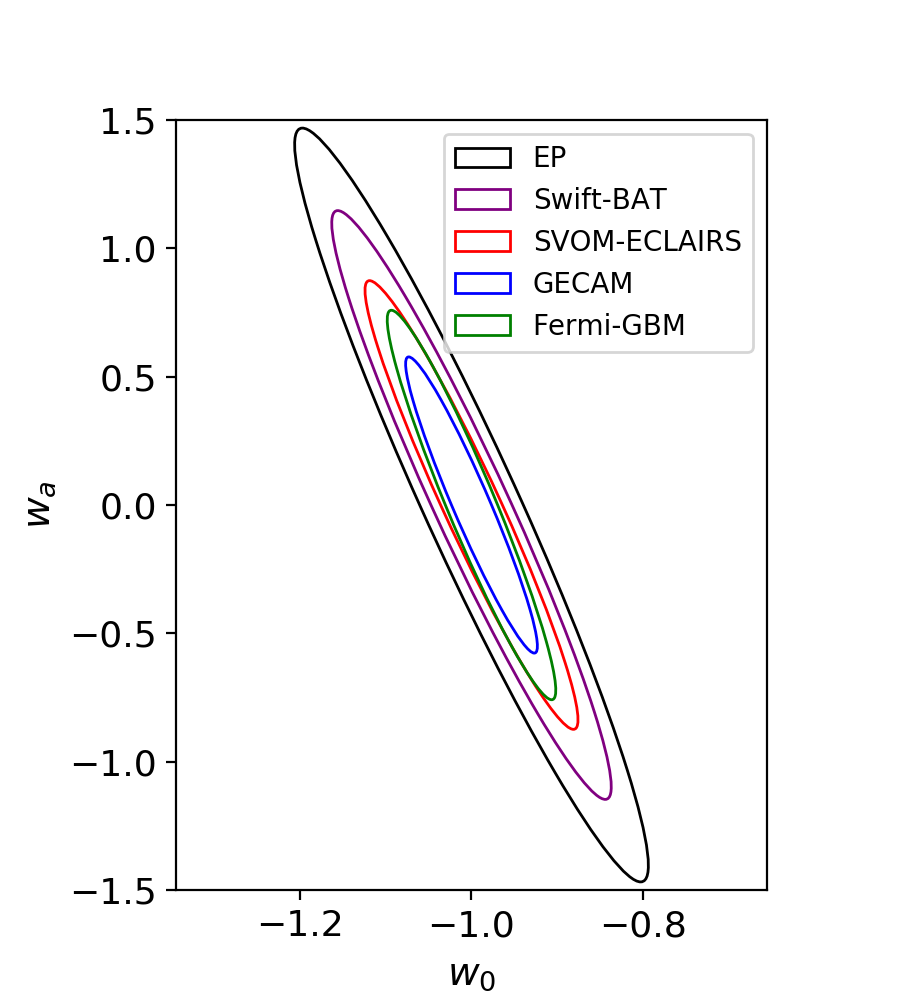
where $C(w_{0},w_{a})$ is the covariance matrix of $w_{0}$ and $w_{a}$. With the large observation area, the results of GECAM and Fermi-GBM are much better than other $\gamma$-ray detectors. For GECAM and CE, we obtain $\Delta w_{0}=0.016-0.051$, $\Delta w_{a}=0.119-0.380$ and $\mathrm{FoM}=171-1732$, for Fermi-GBM, the results are $\Delta w_{0}=0.020-0.065$, $\Delta w_{a}=0.157-0.499$ and $\mathrm{FoM}=100-1009$. These results are comparable with the detection abilities of SNIa and BAO methods in the long-term (Stage IV) projects, which are $\mathrm{FoM}\sim 300$ for SNIa method and $\mathrm{FoM}\sim 100$ for BAO method (Albrecht et al., 2006; Zhao et al., 2011). We can also see that the ET has poor ability of constraining $w_{0}$ and $w_{a}$ due to its low observation limit. In Fig. 6, the corresponding two-dimensional 1-$\sigma$ uncertainty contours of these multi-messenger observations with ET and CE are plotted, and in each figure, we compare the results with four different $\gamma$-ray detectors. For the case of GECAM, the constraints of dark energy parameters are significantly more stringent than other three $\gamma$-ray detectors due to its large observation areas. The results of CEET and CE2ET are not showed here because their shapes are very similar with the results with CE. Our results roughly match the results of Zhao & Wen (2018), but using a much more quantitative BNS sample.

References

- Abbott et al. (2016a) Abbott, B. P., Abbott, R., Abbott, T. D., et al. 2016, Phys. Rev. Lett., 116, 061102
- Abbott et al. (2016b) Abbott, B. P., Abbott, R., Abbott, T. D., et al. 2016, Phys. Rev. Lett., 116, 241103
- Abbott et al. (2016c) Abbott, B. P., Abbott, R., Abbott, T. D., et al. 2016, Phys. Rev. D, 93, 122003
- Abbott et al. (2016d) Abbott, B. P., Abbott, R., Abbott, T. D., et al. 2016, Phys. Rev. X, 6, 041015
- Abbott et al. (2017a) Abbott, B. P., Abbott, R., Abbott, T. D., et al. 2017, Phys. Rev. Lett., 118, 221101
- Abbott et al. (2017b) Abbott, B. P., Abbott, R., Abbott, T. D., et al. 2017, Phys. Rev. Lett., 119, 141101
- Abbott et al. (2017c) Abbott, B. P., Abbott, R., Abbott, T. D., et al. 2017, Phys. Rev. Lett., 119, 161101
- Abbott et al. (2017d) Abbott, B. P., Abbott, R., Abbott, T. D., et al. 2017, Astrophys. J. Lett., 848, L12
- Abbott et al. (2017e) Abbott, B. P., Abbott, R., Abbott, T. D., et al. 2017, Astrophys. J. Lett., 848, L13
- Abbott et al. (2017f) Abbott, B. P., Abbott, R., Abbott, T. D., et al. 2017, Class. Quant. Grav., 34, 044001
- Abbott et al. (2018) Abbott, B. P., Abbott, R., Abbott, T. D., et al. 2018, Living Reviews in Relativity, 21, 3
- Abbott et al. (2019) Abbott, B. P., Abbott, R., Abbott, T. D., et al. 2019, Phys. Rev. X, 9, 031040
- Abbott et al. (2020a) Abbott, B. P., Abbott, R., Abbott, T. D., et al. 2020, Astrophys. J. Lett., 892, L3
- Abbott et al. (2020b) Abbott, R., Abbott, T. D., Abraham, S., et al. 2020, Astrophys. J. Lett., 896, L44
- Abbott et al. (2020c) Abbott, R., Abbott, T. D., Abraham, S., et al. 2020, Phys. Rev. Lett., 125, 101102
- Abbott et al. (2020d) Abbott, R., Abbott, T. D., Abraham, S., et al. 2020, arXiv preprint arXiv:2010.14527
- Abbott et al. (2020e) Abbott, R., Abbott, T. D., Abraham, S., et al. 2020, arXiv preprint arXiv:2010.14533
- Abernathy et al. (2011) Abernathy, M., Acernese, F., Ajith, P., et al. Einstein gravitational wave Telescope conceptual design study[J]. 2011.
- Albrecht et al. (2006) Albrecht, A., Bernstein, G., Cahn, R. et al., Report of the Dark Energy Task Force, arXiv:astro-ph/0609591.
- Alexander et al. (2018) Alexander, K. D., Margutti, R., Blanchard, P. K., et al. 2018, Astrophys. J., 863, L18
- Arcavi (2017) Arcavi, I. 2017, Nature, 551, 64
- Belgacem et al. (2019) Belgacem, E., Dirian, Y., Foffa, S., et al. 2019, JCAP, 08, 015
- Berger (2014) Berger, E. 2014, Annu. Rev. Astron. Astrophys., 52, 43
- Blair et al. (2015) Blair, D., Ju, L., Zhao, C. N., et al. 2015, Science China Physics, Mechanics & Astronomy, 58, 120402
- Blanchet (2002) Blanchet, L. 2002, Living Reviews in Relativity, 5, 3
- Blanchet et al. (2002) Blanchet, L., Faye, G., Iyer, B. R. & Joguet, B. 2002, Phys. Rev. D, 65, 061501
- Blanchet et al. (2004a) Blanchet, L., Damour, T. & Esposito-Farese, G. 2004, Phys. Rev. D, 69, 124007
- Blanchet et al. (2004b) Blanchet, L., Damour, T., Esposito-Farese, G. & Iyer, B. R. 2004, Phys. Rev. Lett.. 93, 091101
- Blanchet & Iyer (2005) Blanchet, L., & Iyer B. R. 2005, Phys. Rev. D71, 024004
- Chen et al. (2018) Chen, H. Y., Fishbach, M., & Holz, D. E. 2018, Nature, 526, 545
- Chen (2020) Chen, H. Y. 2020, Phys. Rev. Lett., 125, 201301
- Chevallier & Polarski (2001) Chevallier, M., & Polarski, D. 2001, Int. J. Mod. Phys. D, 10, 213
- Chu et al. (2016) Chu, Q., Howell, E. J., Rowlinson, A., et al. 2016, Mon. Not. Roy. Astron. Soc., 459, 121
- Copeland et al. (2006) Copeland, E. J., Sami M. & Tsujikawa, S., 2006, Int. J. Mod. Phys. D, 15, 11
- Coulter et al. (2017) Coulter, D. A., Foley, R. J., Kilpatrick, C. D., et al. 2017, Science, 358, 1556
- Cutler et al. (1993) Cutler, C., Apostolatos, T. A., Bildsten, L., et al. 1993, Phys. Rev. Lett., 70, 2984.
- Damour et al. (2001) Damour, T., Jaranowski, P. & Schäfer, G. 2001, Phys. Lett. B, 513, 147
- Dwyer et al. (2015) Dwyer, S., Sigg, D., Ballmer, S. W., et al. 2015, Phys. Rev. D, 91, 082001
- Eichler et al. (1989) Eichler, D., Livio, M., Piran, T. & Schramm, D. N. 1989, Nature, 349, 126
- Eisenstein et al. (2005) Eisenstein, D. J., Zehavi, I., Hogg, D. W., et al. 2005, Astrophys. J., 633, 560
- Erratum (2005) Erratum ibid. D, 71, 129902 (2005)
- Essick et al. (2017) Essick, R., Vitale, S. & Evans, M. 2017, Phys. Rev. D, 96, 084004
- Evans et al. (2017) Evans, P. A., Cenko, S. B., Kennea, J. A., et al., 2017, Science, 358, 1565
- Fishbach et al. (2019) Fishbach, M., Gray, R., Hernandez, I. M., et al. 2019, Astrophys. J. Lett., 871, L13
- Granot et al. (2002) Granot, J., Panaitescu, A., Kumar, O., & Woosley, S. E. 2002, Astrophys. J., 570, L61
- Gehrels et al. (2004) Gehrels, N., Chincarini, G., Giommi, P., et al. 2004, Astrophys. J., 611, 1005
- Ghirlanda et al. (2019) Ghirlanda, G., Salafia, O. S., Paragi, Z., et al. 2019, Science, 363, 968
- Goldstein et al. (2017) Goldstein, A., Veres, P., Burns, E., et al. 2017, Astrophys. J. Lett., 848, L14
- Götz et al. (2014) Götz, D., Osborne, J., Cordier, B., et al. 2014, Proc. SPIE, 9144, 914423
- Gray et al. (2020) Gray, R., Hernandez, I. M., Qi, H., et al. 2020, Phys. Rev. D, 101, 122001
- Gupta et al. (2019) Gupta, A., Fox, D., Sathyaprakash, B. S. & Schutz, B. F., 2019, Astrophys. J., 886, 71
- Hicken et al. (2009) Hicken, M., Wood-Vasey, W. M., Blondin, S., et al. 2009, Astrophys. J., 700, 1097
- Holz & Hughes (2005) Holz, D. E., & Hughes, S. A. 2005, Astrophys. J., 629, 15
- Ioka & Nakamura (2019) Ioka, K., & Nakamura, T. 2019, Mon. Not. Roy. Astron. Soc., 487, 4884
- Itoh et al. (2001) Itoh, Y., Futamase T., & Asada, H. 2001, Phys. Rev. D, 63, 064038
- Itoh & Futamase (2003) Itoh, Y. & Futamase, T. 2003, Phys. Rev. D, 68, 121501
- Itoh (2004a) Itoh, Y. 2004, Phys. Rev. D, 69, 064018
- Itoh (2004b) Itoh, Y. 2004, Class. Quant. Grav.21, S529
- Ivezić et al. (2019) Ivezić, Ž., Kahn, S. M., Tyson, J. A., et al. 2019, Astrophys. J., 873, 111
- Jaranowski et al. (1998) Jaranowski, P., Krolak, A. & Schutz, B. F. 1998, Phys. Rev. D, 58, 063001
- Kilbinger et al. (2009) Kilbinger, M., Benabed, K., Guy, J., et al. 2009, A&A, 497, 677
- Kiziltan et al. (2013) Kiziltan, B., Kottas, A., De Yoreo, M., & Thorsett, S. E. 2013, Astrophys. J., 778, 66
- Komatsu et al. (2009) Komatsu, E., Dunkley, J., Nolta, M. R., et al. 2009, Astrophys. J. Suppl. Ser., 180, 330
- Kowalski et al. (2008) Kowalski, M., Rubin, D., Aldering, G., et al. 2008, Astrophys. J., 686, 749
- Lazzati et al. (2017) Lazzati, D., Deich, A., Morsony, B. J., & Miller, M. C. 2017, Mon. Not. Roy. Astron. Soc., 471, 1652
- Lazzati et al. (2018) Lazzati, D., Perna, R., Morsony, B. J., et al. 2018, Phys. Rev. Lett., 120,241103
- LIGO Scientific Collaboration (2016) LIGO Scientific Collaboration 2016, The LSC-Virgo White Paper on Instrument Science (2016-2017 edition)
- LIGO Collaboration et al. (2017) LIGO Scientific Collaboration, Virgo Collaboration, 1M2H Collaboration, et al. 2017, Nature, 551, 85
- LSC et al. (2017) LIGO Scientific, Virgo, Fermi GBM, INTEGRAL, IceCube, IPN, Insight-Hxmt, et al. 2017, Astrophys. J. Lett., 848, L12
- Li & Paczyński (1998) Li, L. X., & Paczyński, B. 1998, Astrophys. J. Lett., 507, L59
- Meegan et al. (2009) Meegan, C., Lichti, G., Bhat, P. N., et al. 2009, Astrophys. J., 702, 791
- Metzger (2017) Metzger, B. D. 2017, Living reviews in relativity, 20, 3
- Mészáros & Rees (1999) Mészáros, P., & Martin J. R. 1999, Mon. Not. Roy. Astron. Soc., 306, L39
- Mooley et al. (2018) Mooley, K. P., Nakar, E., Hotokezaka, K., et al. 2018, Nature, 554, 207
- Mortlock et al. (2019) Mortlock, D. J., Feeney, S. M., Peiris, H. V., et al. 2019, Phys. Rev. D, 10, 103523
- Nakar et al. (2002) Nakar, E., Piran, T., & Granot, J. 2002, Astrophys. J., 579, 699
- Narayan et al. (1992) Narayan, R., Paczynski B. & Piran T. 1992, Astrophys. J. Lett., 395, L83
- Paczynski (1986) Paczynski, B. 1986, Astrophys. J. Lett., 308, L43
- Percival et al. (2007) Percival, W. J., Cole, S., Eisenstein, D. J., et al. 2007, Mon. Not. Roy. Astron. Soc., 381, 1053
- Percival et al. (2010) Percival, W. J., Reid, B. A., Eisenstein, D. J., et al. 2010, Mon. Not. Roy. Astron. Soc., 401, 2148
- Planck Collaboration XIII (2016) Planck Collaboration, Ade, P. A. R., Aghanim, N., et al. 2016, A&A, 594, A13
- Preece et al. (2000) Preece, R. D., Briggs, M. S., Mallozzi, R. S., et al. 2000, Astrophys. J. Suppl. Ser., 126, 19
- Punturo et al. (2010) Punturo, M., Abernathy, M., Acernese, F., et al. 2010, Class. Quant. Grav., 27, 194002
- Rosswog (2005) Rosswog, S., 2005, Astrophys. J.. 634, 1202
- Rosswog (2013) Rosswog, S., 2013, Nature, 500, 535
- Sari et al. (1998) Sari, R., Piran, T. & Narayan, J. P. 1998, Astrophys. J., 497, L17
- Sathyaprakash & Schutz (2009) Sathyaprakash, B. S. & Schutz, B. F. 2009, Living Rev. Relativity, 12, 2
- Sathyaprakash et al. (2010) Sathyaprakash, B. S., Schutz, B. F., & Van Den Broeck, C. 2010, Class. Quant. Grav., 27, 215006
- Savchenko et al. (2017) Savchenko, V., Ferrigno, C., Kuulkers, E., et al. 2017, Astrophys. J. Lett., 848, L15
- Schrabback et al. (2010) Schrabback, T., Hartlap, J., Joachimi, B., et al. 2010, A&A, 516, A63
- Schutz (1986) Schutz, B. F., 1986, Nature, 323, 310
- Song et al. (2019) Song H. R., Ai S. K., Wang M. H., et al. 2019, Astrophys. J. Lett., 881, L40
- Soares-Santos et al. (2017) Soares-Santos, M., Holz, D. E., Annis, J., et al. 2017, Astrophys. J. Lett., 848, L16
- Soares-Santos et al. (2019) Soares-Santos, M., Palmese, A., Hartley, W., et al. 2019, Astrophys. J. Lett., 876, L7
- Sun et al. (2015) Sun, H., Zhang, B., & Li, Z. 2015, Astrophys. J., 812, 33
- Tanvir et al. (2017) Tanvir, N. R., Levan, Astron. J., Gonzalez-Fernandez, C., et al. 2017, Astrophys. J. Lett., 848, L27
- Tan & Yu (2018) Tan, W. W. & Yu, Y. W. 2018, Astrophys. J., 902, 83
- Tanvir et al. (2013) Tanvir, N. R., Levan, A. J., Fruchter, A. S., et al. 2013, Nature, 500, 547-549
- Troja et al. (2018) Troja, E., Piro, L., Ryan, G., et al. 2018, Mon. Not. Roy. Astron. Soc., 487, L18
- Unnikrishnan (2013) Unnikrishnan, C. S. 2013, Int. J. Mod. Phys. D, 22, 1341010
- Virgili et al. (2011) Virgili, F. J., Zhang, B., O’Brien, P.& Troja, E., 2011, Astrophys. J., 727,109
- Valenti et al. (2017) Valenti, S., David, J., Yang, S., et al. 2017, Astrophys. J. Lett., 848, L24
- Vitale & Evans (2017) Vitale, S. & Evans, M. 2017, Phys. Rev. D, 95, 064052
- Wanderman & Piran (2015) Wanderman, D. & Piran, T. 2015, Mon. Not. Roy. Astron. Soc., 448,3026
- Wang et al. (2020) Wang, B., Zhu, Z. Y., Li, A. & Zhao, W., 2020, Astrophys. J. Suppl. Ser., 250, 6
- Wang & Wang (2019) Wang, Y. Y. & Wang, F. Y. 2019, Astrophys. J., 873,39
- Wen & Chen (2010) Wen, L. & Chen, Y. 2010, Phys. Rev. D, 81, 082001
- Weinberg (2008) Weinberg, S. 2008, Cosmology, Oxford University Press
- Yan et al. (2020) Yan, C. S., Zhao, W., & Lu, Y. J., 2020, Astrophys. J., 889, 79
- Yonetoku et al. (2004) Yonetoku, D., Murakami, T., Nakamura, T., et al. 2004, Astrophys. J., 609, 935
- Yu et al. (2020) Yu, J. M., Wang, Y., Zhao, W. & Lu, Y. J. 2020, Mon. Not. Roy. Astron. Soc., 498, 1786
- Yuan et al. (2018) Yuan, W., Zhang, C., Chen, Y., et al. 2018, Scientia Sinica Physica, Mechanica & Astronomica, 48, 039502
- Yuksel et al. (2008) Yuksel, H., Kistler, M. D., Beacom, J. F., et al. 2008, Astrophys. J., 683,L5
- Zhao et al. (2018) Zhao, W., Wright, B. S. & Li, B., 2018, JCAP, 10, 052
- Zhao et al. (2011) Zhao, W., van den Broeck, C., Baskaran, D., & Li, T. G. F. 2011, Phys. Rev. D, 83, 023005
- Zhao & Santos (2019) Zhao, W. & Santos, L. 2019, JCAP, 11, 009
- Zhao & Wen (2018) Zhao, W. & Wen, L. 2018, Phys. Rev. D, 97, 064031
- Zhang & Mészáros (2002) Zhang, B. & Mészáros, P. 2002, Astrophys. J., 571, 876
- Zhang et al. (2017) Zhang, X., Yu, J., Liu, T., Zhao, W. & Wang, A. Z. 2017, Phys. Rev. D, 95, 124008
- Zhang et al. (2018) Zhang, D. L., Li, X. Q., Xiong, S. L., et al. 2018, arXiv preprint arXiv:1804.04499
- Zhang & Wang (2018) Zhang, G. Q. & Wang, F. Y. 2018, Astrophys. J., 852,1
- Zou et al. (2007) Zou, Y. C., We, X. F. & Dai, Z. G. 2007, Astron. Astrophys., 461, 115