Multi-facet Contextual Bandits: A Neural Network Perspective

Yikun Ban University of Illinois at Urbana-Champaign [email protected] , Jingrui He University of Illinois at Urbana-Champaign [email protected] and Curtiss B. Cook Mayo Clinic Arizona [email protected]

(2021)

Abstract.

Contextual multi-armed bandit has shown to be an effective tool in recommender systems. In this paper, we study a novel problem of multi-facet bandits involving a group of bandits, each characterizing the users’ needs from one unique aspect. In each round, for the given user, we need to select one arm from each bandit, such that the combination of all arms maximizes the final reward. This problem can find immediate applications in E-commerce, healthcare, etc. To address this problem, we propose a novel algorithm, named MuFasa, which utilizes an assembled neural network to jointly learn the underlying reward functions of multiple bandits. It estimates an Upper Confidence Bound (UCB) linked with the expected reward to balance between exploitation and exploration. Under mild assumptions, we provide the regret analysis of MuFasa. It can achieve the near-optimal $\widetilde{\mathcal{O}}((K+1)\sqrt{T})$ regret bound where $K$ is the number of bandits and $T$ is the number of played rounds. Furthermore, we conduct extensive experiments to show that MuFasa outperforms strong baselines on real-world data sets.

Contextual Bandits; Neural Network; Regret Analysis

^†^†ccs: Information systems Personalization^†^†ccs: Information systems Display advertising^†^†ccs: Theory of computation Online learning algorithms^†^†journalyear: 2021^†^†copyright: acmcopyright^†^†conference: Proceedings of the 27th ACM SIGKDD Conference on Knowledge Discovery and Data Mining; August 14–18, 2021; Virtual Event, Singapore^†^†booktitle: Proceedings of the 27th ACM SIGKDD Conference on Knowledge Discovery and Data Mining (KDD ’21), August 14–18, 2021, Virtual Event, Singapore^†^†price: 15.00^†^†doi: 10.1145/3447548.3467299^†^†isbn: 978-1-4503-8332-5/21/08

1. introduction

The personalized recommendation is ubiquitous in web applications. Conventional approaches that rely on sufficient historical records, e.g., collaborative filtering (Su and Khoshgoftaar, 2009; Zhou et al., 2020b), have proven successful both theoretically and empirically. However, with the cold-start problem and the rapid change of the recommendation content, these methods might render sub-optimal performance (Li et al., 2010; Gentile et al., 2014). To solve the dilemma between the exploitation of historical data and the exploration of new information, Multi-Armed Bandit (MAB) (Langford and Zhang, 2008; Auer et al., 2002a; Abbasi-Yadkori et al., 2011; Auer et al., 2002b; Ban and He, 2020) turns out to be an effective tool, which has been adapted to personalized recommendation (Li et al., 2010; Gentile et al., 2014), online advertising (Wu et al., 2016), clinical trials (Durand et al., 2018; Bastani and Bayati, 2020), etc.

In the conventional contextual bandit problem setting (Li et al., 2010), i.e., single MAB, the learner is presented with a set of arms in each round, where each arm is represented by a feature vector. Then the learner needs to select and play one arm to receive the corresponding reward that is drawn from an unknown distribution with an unknown mean. To achieve the goal of maximizing the accumulated rewards, the learner needs to consider the arms with the best historical feedback as well as the new arms for potential gains. The single MAB problem has been well studied in various settings. With respect to the reward function, one research direction (Li et al., 2010; Abbasi-Yadkori et al., 2011; Dimakopoulou et al., 2019; Gentile et al., 2014; Li et al., 2016a) assumes that the expected reward is linear with respect to the arm’s feature vector. However, in many real applications, this assumption fails to hold. Thus many exiting works turn to focus on the nonlinear or nonparametric bandits (Srinivas et al., 2009; Bubeck et al., 2011) with mild assumptions such as the Lipschitz continuous property (Bubeck et al., 2011) or embedding in Reproducing Kernel Hilbert Space (Valko et al., 2013; Deshmukh et al., 2017). Furthermore, the single MAB problem has been extended to best arm identification (Auer et al., 2002a; Audibert and Bubeck, 2010), outlier arm identification (Gentile et al., 2017; Ban and He, 2020), Top-K arm problems (Buccapatnam et al., 2013), and so on.

In this paper, we define and study a novel problem of multi-facet contextual bandits. In this problem, the users’ needs are characterized from multiple aspects, each associated with one bandit. Consider a task consisting of $K$ bandits, where each bandit presents a set of arms separately and the learner needs to choose and play one arm from each bandit. Therefore, a total of $K$ arms are played in one round. In accordance with the standard bandit problem, the learner can observe a reward after playing one arm from the bandit, which we call "sub-reward", and thus $K$ sub-rewards are received in total. In addition, a reward that is a function with respect to these $K$ sub-rewards, called "final reward", is observed to represent the overall feedback with respect to the $K$ selected arms. Note that the functions of final reward and $K$ sub-rewards are allowed to be either linear or non-linear. The goal of the learner in the multi-facet bandit problem is to maximize the final rewards of all the played rounds.

This problem finds many applications in real-world problems. For instance, in the recommender system, instead of the single item recommendation, an E-commerce company launches a promotion campaign, which sells collections of multiple types of products such as snacks, toiletries, and beverages. Each type of item can be formulated as a multi-armed bandit and the learner aims to select the best combination of snack, toiletry, and beverage. As a result, the final reward is the review of this combined recommendation, while the sub-reward is the review for a particular product . This problem also exists in healthcare. For a diabetes patient, the doctor usually provides a comprehensive recommendation including medication, daily diet, and exercise, where each type has several options. Here, the final reward can be set as the change of key biomarkers for diabetes (e.g., HbA1c) and the sub-reward can be the direct impact of each type of recommendation (e.g., blood pressure change for a medicine).

A major challenge of the proposed multi-facet bandit problem is the partial availability of sub-rewards, as not every sub-reward is easy to observe. For example, regarding the combined recommendation of E-commerce, the user may rate the combination but not individual items; regarding the comprehensive recommendation for a diabetes patient, some sub-rewards can be difficult to measure (e.g., the impact of low-calorie diets on the patient’s overall health conditions). Therefore, in our work, we allow only a subset of all sub-rewards to be observed in each round, which increases the flexibility of our proposed framework.

To address these challenges, we aim to learn the mappings from the selected $K$ arms (one from each bandit) to the final rewards, incorporating two crucial factors: (1) the collaborative relations exist among these bandits as they formulate the aspects from one same user; (2) the bandits contribute to the task with various weights because some aspects (bandits) are decisive while some maybe not. Hence, we propose a novel algorithm, MuFasa, to learn $K$ bandits jointly. It utilizes an assembled neural networks to learn the final reward function combined with $K$ bandits. Although the neural networks have been adapted to the bandit problem (Riquelme et al., 2018; Zahavy and Mannor, 2019; Zhou et al., 2020a), they are designed for the single bandit with one selected arm and one reward in each round. To balance the exploitation and exploration of arm sets, we provide a comprehensive upper confidence bound based on the assembled network linking the predicted reward with the expected reward. When the sub-rewards are partially available, we introduce a new approach to leverage them to train bandits jointly. Furthermore, we carry out the theoretical analysis of MuFasa and prove a near-optimal regret bound under mild assumptions. Our major contributions can be summarized as follows:

(1) Problem. We introduce the problem of multi-facet contextual bandits to characterize the users’ needs from multiple aspects, which can find immediate applications in E-commerce, healthcare, etc.

(2) Algorithm. We propose a novel algorithm, MuFasa, which exploits the final reward and up to $K$ sub-rewards to train the assembled neural networks and explores potential arm sets with a UCB-based strategy.

(3) Theoretical analysis. Under mild assumptions, we provide the upper confidence bounds for a neural network and the assembled neural networks. Then, we prove that MuFasa can achieve the $\widetilde{\mathcal{O}}((K+1)\sqrt{T})$ regret bound, which is near-optimal compared to a single contextual bandit.

(4) Empirical performance. We conduct extensive experiments to show the effectiveness of MuFasa, which outperforms strong baselines on real-world data sets even with partial sub-rewards.

2. related work

Multi-armed bandit. The multi-armed bandit was first introduced by (Thompson, 1933) and then further studied by many works that succeeded in both theory and practice such as $\epsilon$ -greedy (Langford and Zhang, 2008), Thompson sampling(Agrawal and Goyal, 2013), and upper confidence bound (Auer et al., 2002a). In the contrast with traditional bandits (Auer et al., 2002a; Ban and He, 2020), the contextual bandit (Li et al., 2010; Abbasi-Yadkori et al., 2011; Wu et al., 2016) has the better representation capacity where each arm is represented by a context vector instead of a scalar to infer the reward. Among them, the linear contextual bandits are extensively studied and many of them use the UCB strategy, achieving $\widetilde{\mathcal{O}}(\sqrt{T})$ regret bound (Abbasi-Yadkori et al., 2011; Gentile et al., 2014; Ban and He, 2021). To further generalize the reward function, many works use a nonlinear regression model drawn from the reproducing kernel Hilbert space to learn the mapping from contexts to rewards such as the kernel-based methods (Deshmukh et al., 2017; Valko et al., 2013).

Neural bandits. The authors of (Allesiardo et al., 2014) use a neural work to model an arm and then applied $\epsilon$ -greedy strategy to select an arm. In contrast, MuFasa utilizes a UCB-based strategy working on $K$ bandits instead of one set of arms. In addition, the Thompson sampling has been combined with deep neural networks (Lipton et al., 2018; Azizzadenesheli et al., 2018; Riquelme et al., 2018; Zahavy and Mannor, 2019). For instance, (Riquelme et al., 2018; Zahavy and Mannor, 2019) regard the last layer of the neural network as the embeddings of contexts and then apply the Thompson sampling to play an arm in each round. NeuUCB (Zhou et al., 2020a) first uses the UCB-based approach constructed on a fully-connected neural network, while it only fits on the single bandit with one set of arms. On the contrary, MuFasa constructs an assembled neural networks to learn $K$ bandits jointly. Deep neural network in multi-view learning has been well-studied (Zhou et al., 2015, 2020c; Fu et al., 2020; Zheng et al., 2021; Jing et al., 2021), to extract useful information among multiple sources, which inspires one of the core ideas of MuFasa.

Other variant bandit setting. In the non-contextual bandit, a number of works (Chen et al., 2013, 2016; Liu et al., 2011) study playing $K$ arms at the same time in a single bandit, while these approaches have limited representation power in the recommender system. The most similar setting is the contextual combinatorial MAB problem(Qin et al., 2014; Li et al., 2016b), where the learner tends to choose the optimal subset of arms with certain constraints like the $K$ -size. One key difference is that all the arms are from the same single bandit where only one reward function exists. On the contrary, in the multi-faced bandits, the selected $K$ arms come from $K$ different bandits with $K$ different reward functions and the sub-rewards are allowed to be partially available. There is another line of works (Gentile et al., 2014; Li et al., 2016a; Ban and He, 2021) for bandit clustering, where a bandit is constructed for each user. They try to leverage the dependency among users to improve the recommendation performance. However, in these works, they still play one arm in each round and the reward function is required to be linear.

3. Problem Definition

In this section, we formulate the problem of multi-facet bandits, with a total of $K$ bandits, where the learner aims to select the optimal set of $K$ arms in each round, in order to maximize the final accumulated rewards.

Suppose there are $T$ rounds altogether. In each round $t\in[T]$ ( $[T]=\{1,\dots,T\}$ ), the learner is faced with $K$ bandits, and each bandit $k\in[K]$ has a set of arms $\mathbf{X}^{k}_{t}=\{\mathbf{x}^{k}_{t,1},\dots,\mathbf{x}^{k}_{t,n_{k}}\}$ , where $|\mathbf{X}^{k}_{t}|=n_{k}$ is the number of arms in this bandit. In the bandit $k$ , for each arm $\mathbf{x}^{k}_{t,i}\in\mathbf{X}^{k}_{t}$ , it is represented by a $d_{k}$ -dimensional feature vector and we assume $\|\mathbf{x}^{k}_{t,i}\|_{2}\leq 1$ . Subsequently, in each round $t$ , the learner will observe $K$ arm sets $\{\mathbf{X}^{k}_{t}\}_{k=1}^{K}$ and thus a total of $\sum_{k=1}^{K}n_{k}$ arms. As only one arm can be played within each bandit, the learner needs to select and play $K$ arms denoted as $\mathbf{X}_{t}=\{\mathbf{x}^{1}_{t},\dots,\mathbf{x}^{k}_{t},\dots,\mathbf{x}^{K}_{t}\}$ in which $\mathbf{x}_{t}^{k}\in\mathbf{X}_{t}$ represents the selected arm from $\mathbf{X}^{k}_{t}$ .

Once the selected arm $\mathbf{x}^{k}_{t}$ is played for bandit $k$ , a sub-reward $r^{k}_{t}$ will be received to represent the feedback of this play for bandit $k$ separately. The sub-reward is assumed to be governed by an unknown reward function:

r^{k}_{t}(\mathbf{x}^{k}_{t})=h_{k}(\mathbf{x}^{k}_{t}).

where $h_{k}$ can be either a linear (Li et al., 2010; Abbasi-Yadkori et al., 2011) or non-linear reward function (Deshmukh et al., 2017; Valko et al., 2013). As a result, in each round $t$ , the learner needs to play $K$ arms in $\mathbf{X}_{t}$ and then receive $K$ sub-rewards denoted by $\mathbf{r}_{t}=\{r^{1}_{t},\dots,r^{k}_{t},\dots,r^{K}_{t}\}$ .

As the $K$ bandits characterize the users’ needs from various aspects, after playing $K$ arms in each round $t$ , a final reward $R_{t}$ will be received to represent the overall feedback of the group of $K$ bandits. The final reward $R_{t}$ is considered to be governed by an unknown function with respect to $\mathbf{r}_{t}$ :

R_{t}(\mathbf{r}_{t})=H\left(\left(h_{1}(\mathbf{x}_{t}^{1}),\dots,h_{k}(\mathbf{x}_{t}^{k})\dots,h_{K}(\mathbf{x}_{t}^{K})\right)\right)+\epsilon_{t}.

where $\epsilon_{t}$ is a noise drawn from a Gaussian distribution with zero mean. In our analysis, we make the following assumptions regarding $h_{k}$ and $H(\text{vec}(\mathbf{r}_{t}))$ :

(1)

If $\mathbf{x}_{t}^{k}=\mathbf{0}$ , then $h(\mathbf{x}_{t}^{k})=0$ ; If $\text{vec}(\mathbf{r}_{t})=(0,\dots,0)$ , then $H(\text{vec}(\mathbf{r}_{t}))=0$ .

(2)

$\bar{C}$ -Lipschitz continuity. $H(\text{vec}(\mathbf{r}_{t}))$ is assumed to be $\bar{C}$ -Lipschitz continuous with respect to the $\mathbf{r}_{t}$ . Formally, there exists a constant $\bar{C}>0$ such that

|H(\text{vec}(\mathbf{r}_{t}))-H(\text{vec}(\mathbf{r}_{t}^{\prime}))|\leq\bar{C}\sqrt{\sum_{k\in K}[r_{t}^{k}-{r_{t}^{k}}^{\prime}]^{2}}.

Both assumptions are mild. For (1), if the input is zero, then the reward should also be zero. For (2), the Lipschitz continuity can be applied to many real-world applications. For the convenience of presentation, given any set of selected $K$ arms $\mathbf{X}_{t}$ , we denote the expectation of $R_{t}$ by:

(1)

\mathcal{H}(\mathbf{X}_{t})=\mathbb{E}[R_{t}|\mathbf{X}_{t}]=H\left(\left(h_{1}(\mathbf{x}_{t}^{1}),\dots,h_{k}(\mathbf{x}_{t}^{k})\dots,h_{K}(\mathbf{x}_{t}^{K})\right)\right).

Recall that in multi-facet bandits, the learner aims to select the optimal $K$ arms with the maximal final reward $R_{t}^{\ast}$ in each round. First, we need to identify all possible combinations of $K$ arms, denoted by

(2)

\mathbf{S}_{t}=\{(\mathbf{x}^{1}_{t},\dots,\mathbf{x}^{k}_{t},\dots,\mathbf{x}^{K}_{t})\ |\ \mathbf{x}^{k}_{t}\in\mathbf{X}^{k}_{t},k\in[K]\},

where $|\mathbf{S}_{t}|=\prod_{k=1}^{K}n_{k}$ because bandit $k$ has $n_{k}$ arms for each $k\in[K]$ . Thus, the regret of multi-facet bandit problem is defined as

	Reg	$\displaystyle=\mathbb{E}[\sum_{t=1}^{T}(R_{t}^{\ast}-R_{t})]$
		$\displaystyle=\sum_{t=1}^{T}\left(\mathcal{H}(\mathbf{X}_{t}^{\ast})-\mathcal{H}(\mathbf{X}_{t})\right),$

where $\mathbf{X}_{t}^{\ast}=\arg\max_{\mathbf{X}_{t}\in\mathbf{S}_{t}}\mathcal{H}(\mathbf{X}_{t})$ . Therefore, our goal is to design a bandit algorithm to select $K$ arms every round in order to minimize the regret. We use the standard $\mathcal{O}$ to hide constants and $\widetilde{\mathcal{O}}$ to hide logarithm.

Availability of sub-rewards. In this framework, the final $R_{t}$ is required to be known, while the sub-rewards $\mathbf{r}_{t}$ are allowed to be partially available. Because the feedback of some bandits cannot be directly measured or is simply not available in a real problem. This increases the flexibility of our proposed framework.

More specifically, in each round $t$ , ideally, the learner is able to receive $K+1$ rewards including $K$ sub-rewards $\{r^{1}_{t},\dots,r^{K}_{t}\}$ and a final reward $R_{t}$ . As the final reward is the integral feedback of the entire group of bandits and reflects how the bandits affect each other, $R_{t}$ is required to be known. However, the $K$ sub-rewards are allowed to be partially available, because not every sub-reward is easy to obtain or can be measured accurately.

This is a new challenge in the multi-facet bandit problem. Thus, to learn $\mathcal{H}$ , the designed bandit algorithm is required to handle the partial availability of sub-rewards.

4. Proposed Algorithm

In this section, we introduce the proposed algorithm, MuFasa. The presentation of MuFasa is divided into three parts. First, we present the neural network model used in MuFasa; Second, we detail how to collect training samples to train the model in each round; In the end, we describe the UCB-based arm selection criterion and summarize the workflow of MuFasa.

4.1. Neural network model

To learn the reward function $\mathcal{H}$ , we use $K+1$ fully-connected neural networks to learn $K$ bandits jointly, where a neural network $f_{k}$ is built for each bandit $k\in[K]$ to learn its reward function $h_{k}$ , and a shared neural network $F$ is constructed to learn the mapping from the $K$ neural networks $(f_{1},\dots,f_{K})$ to the final reward $R_{t}$ .

First, in round $t$ , for each bandit $k\in[K]$ , given any context vector $\mathbf{x}^{k}_{t}\in\mathbb{R}^{d_{k}}$ , we use a $L_{1}$ -layer fully-connected network to learn $h_{k}$ , denoted by $f_{k}$ :

f_{k}(\mathbf{x}^{k}_{t};\bm{\theta}^{k})=\sqrt{m_{1}}\mathbf{W}_{L_{1}}\sigma(\mathbf{W}_{L_{1}-1}\sigma(\dots\sigma(\mathbf{W}_{1}\mathbf{x}^{k}_{t}))),

where $\sigma(x)$ is the rectified linear unit (ReLU) activation function. Without loss of generality, we assume each layer has the same width $m_{1}$ for the sake of analysis. Therefore, $\bm{\theta}^{k}=\big{(}\text{vec}(\mathbf{W}_{L_{1}})^{\intercal},\dots,$ $\text{vec}(\mathbf{W}_{1})^{\intercal}\big{)}^{\intercal}$ $\in\mathbb{R}^{P_{1}}$ , where $\mathbf{W}_{1}\in\mathbb{R}^{m_{1}\times d_{k}}$ , $\mathbf{W}_{i}\in\mathbb{R}^{m_{1}\times m_{1}},\forall i\in[1\mathrel{\mathop{\mathchar 58\relax}}L_{1}-1]$ , and $\mathbf{W}_{L_{1}}\in\mathbb{R}^{\widehat{m}\times m_{1}}$ . Note that $f_{k}(\mathbf{x}^{k}_{t};\bm{\theta}^{k})\in\mathbb{R}^{\widehat{m}}$ , where $\widehat{m}$ is set as a tuneable parameter to connect with the following network $F$ . Denote the gradient $\triangledown_{\bm{\theta}^{k}}f_{k}(\mathbf{x}^{k}_{t};\bm{\theta}^{k})$ by $g(\mathbf{x}_{t}^{k};\bm{\theta}^{k})$ .

Next, to learn the final reward function $H$ , we use a $L_{2}$ -layer fully-connected network to combine the outputs of the above $K$ neural networks, denoted by $F$ :

F\left(\mathbf{f}_{t};\bm{\theta}^{\Sigma}\right)=\sqrt{m_{2}}\mathbf{W}_{L_{2}}\sigma(\dots\sigma(\mathbf{W}_{1}(\mathbf{f}_{t})))

where $\mathbf{f}_{t}=\left(f_{1}(\mathbf{x}_{t}^{1};\bm{\theta}^{1})^{\intercal},\dots,f_{K}(\mathbf{x}_{t}^{K};\bm{\theta}^{K})^{\intercal}\right)^{\intercal}\in\mathbb{R}^{\widehat{m}K}$ . Also, we assume that each layer has the same width $m_{2}$ . Therefore, $\bm{\theta}^{\Sigma}=(\text{vec}(\mathbf{W}_{L_{2}})^{\intercal}$ $,\dots,\text{vec}(\mathbf{W}_{1})^{\intercal})^{\intercal}\in\mathbb{R}^{P_{2}}$ , where $\mathbf{W}_{1}\in\mathbb{R}^{m_{2}\times\widehat{m}K}$ , $\mathbf{W}_{i}\in\mathbb{R}^{m_{2}\times m_{2}},\forall i\in[L_{2}-1]$ and $\mathbf{W}_{L_{2}}\in\mathbb{R}^{1\times m_{2}}$ , Denote the gradient $\triangledown_{\bm{\theta}^{\Sigma}}F\left(\mathbf{f}_{t};\bm{\theta}^{\Sigma}\right)$ by $G(\mathbf{f}_{t};\bm{\theta}^{\Sigma})$ .

Therefore, for the convenience of presentation, the whole assembled neural networks can be represented by $\mathcal{F}$ to learn $\mathcal{H}$ (Eq.(6)), given the $K$ selected arms $\mathbf{X}_{t}$ :

\mathcal{F}(\mathbf{X}_{t};\bm{\theta})=\left(F(\cdot;\bm{\theta}^{\Sigma})\circ\left(f_{1}(\cdot;\bm{\theta}^{1}),\dots,f_{K}(\cdot;\bm{\theta}^{K})\right)\right)(\mathbf{X}_{t}),

where $\bm{\theta}=(\bm{\theta}^{\Sigma},\bm{\theta}^{1},\dots,\bm{\theta}^{K})$ .

Initialization. $\bm{\theta}$ is initialized by randomly generating each parameter from the Gaussian distribution. More specifically, for $\bm{\theta}^{k},k\in[K]$ , $\mathbf{W}_{l}$ is set to $\begin{pmatrix}\mathbf{w}&\mathbf{0}\\ \mathbf{0}&\mathbf{w}\end{pmatrix}$ for any $l\in[L_{1}]$ where $\mathbf{w}$ is drawn from $N(0,4/m_{1})$ . For $\bm{\theta}^{\Sigma}$ , $\mathbf{W}_{l}$ is set to $\begin{pmatrix}\mathbf{w}&\mathbf{0}\\ \mathbf{0}&\mathbf{w}\end{pmatrix}$ for any $l\in[L_{2}-1]$ where $\mathbf{w}$ is drawn from $N(0,4/m_{2})$ ; $\mathbf{W}_{L_{2}}$ is set to $(\mathbf{w}^{\intercal},-\mathbf{w}^{\intercal})$ where $\mathbf{w}$ is drawn from $N(0,2/m_{2})$ .

Algorithm 1 MuFasa

\mathcal{F}

T

K

\delta

\eta

J

2:Initialize

\bm{\theta}_{0}=(\bm{\theta}^{\Sigma}_{0},\bm{\theta}^{1}_{0},\dots,\bm{\theta}^{K}_{0})

3:for each

t\in[T]

4: for each bandit

k\in[K]

5: Observe context vectors

\mathbf{X}_{t}^{k}=\{\mathbf{x}_{t,1}^{k},\dots,\mathbf{x}_{t,n_{k}}^{k}\}

6: Collect

\mathbf{S}_{t}

(Eq. (2))

7: Choose

K

arms,

\mathbf{X}_{t}

, by:

\mathbf{X}_{t}=\arg\max_{\mathbf{X}_{t}^{\prime}\in\mathbf{S}_{t}}\bigg{(}\mathcal{F}(\mathbf{X}_{t}^{\prime};\bm{\theta}_{t-1})+\text{UCB}(\mathbf{X}_{t}^{\prime})\bigg{)}.\ \ \ (\ \text{Theorem}\ \ref{theo:ucb}\ )

8: Play

\mathbf{X}_{t}

and observe rewards

R_{t}

and

\mathbf{r}_{t}

9: if

|\mathbf{r}_{t}|=K

then ## sub-rewards are all available.

10:

\bm{\theta}_{t}

GradientDescent_{All}

(

\mathcal{F}

\{\mathbf{X}_{i}\}_{i=1}^{t}

\{R_{i}\}_{i=1}^{t}

\{\mathbf{r}_{i}\}_{i=1}^{t}

J,\eta

)

11: else ## sub-rewards are partially available.

12: Collect

\{\Omega_{i}\}_{i=1}^{t}

( Eq.(4) )

13:

\bm{\theta}_{t}

GradientDescent_{Partial}

(

\mathcal{F}

\{\Omega_{i}\}_{i=1}^{t}

J

\eta

)

14: Update

\text{UCB}(\mathbf{X}_{t}^{\prime})

4.2. Training process

Only with the final reward $R_{t}$ and $K$ selected arms $\mathbf{X}_{t}$ , the training of the neural network model $\mathcal{F}$ is the following minimization problem:

(3)

\min_{\bm{\theta}}\mathcal{L}(\bm{\theta})=\sum_{t=1}^{T}\left(\mathcal{F}(\mathbf{X}_{t};\bm{\theta})-R_{t}\right)^{2}/2+m_{2}\lambda\|\bm{\theta}-\bm{\theta}_{0}\|_{2}^{2}/2.

where $\mathcal{L}(\bm{\theta})$ is essentially $l_{2}$ -regularized square loss function and $\bm{\theta}_{0}$ is the randomly initialized network parameters. However, once the sub-rewards are available, we should use different methods to train $\mathcal{F}$ , in order to leverage more available information. Next, we will elaborate our training methods using the gradient descend.

Collection of training samples. Depending on the availability of sub-rewards, we apply different strategies to update $\bm{\theta}$ in each round. When the sub-rewards are all available, the learner receives one final reward and $K$ sub-rewards. We apply the straightforward way to train each part of $\mathcal{F}$ accordingly based on the corresponding input and the ground-truth rewards in each round, referring to the details in Algorithm 2, where $\widetilde{m}$ in $\mathcal{F}$ should be set as $1$ .

Algorithm 2

GradientDescent_{All}

\mathcal{F}

\{\mathbf{X}_{i}\}_{i=1}^{t}

\{R_{i}\}_{i=1}^{t}

\{\mathbf{r}_{i}\}_{i=1}^{t}

J,\eta

\bm{\theta}_{t}

3:for each

k\in[K]

4: Define

\mathcal{L}(\bm{\theta}^{k})=\sum_{i=1}^{t}\left(f_{k}(\mathbf{x}_{i}^{k};\bm{\theta}^{k})-r_{i}^{k}\right)^{2}/2+m_{1}\lambda\|\bm{\theta}^{k}-\bm{\theta}_{0}\|_{2}^{2}/2

5: for each

j\in[J]

\bm{\theta}^{k}_{j}=\bm{\theta}^{k}_{j-1}-\eta\triangledown\mathcal{L}(\bm{\theta}^{k}_{j-1})

7:Define

\mathcal{L}(\bm{\theta}^{\Sigma})=\sum_{i=1}^{t}\left(F(\text{vec}(\mathbf{r}_{i});\bm{\theta}^{\Sigma})-R_{i}\right)^{2}/2+m_{2}\lambda\|\bm{\theta}^{\Sigma}-\bm{\theta}_{0}\|_{2}^{2}/2

8:for each

j\in[J]

\bm{\theta}^{\Sigma}_{j}=\bm{\theta}^{\Sigma}_{j-1}-\eta\triangledown\mathcal{L}(\bm{\theta}^{\Sigma}_{j-1})

10:return

(\bm{\theta}^{\Sigma}_{J},\bm{\theta}^{1}_{J},\dots,\bm{\theta}^{K}_{J})

Algorithm 3

GradientDescent_{Partial}

\mathcal{F}

\{\Omega_{i}\}_{i=1}^{t}

J,\eta

\bm{\theta}_{t}

3:Define

\mathcal{L}(\bm{\theta})=\sum_{i=1}^{t}\sum_{(\mathbf{X},R)\in\Omega_{i}}\left(\mathcal{F}(\mathbf{X};\bm{\theta})-R\right)^{2}/2+m_{2}\lambda\|\bm{\theta}-\bm{\theta}_{0}\|_{2}^{2}/2

4:for each

j\in[J]

\bm{\theta}_{j}=\bm{\theta}_{j-1}-\eta\triangledown\mathcal{L}(\bm{\theta}_{j-1})

6:return

\bm{\theta}_{j}

However, when the sub-rewards are partially available, the above method is not valid anymore because the bandits without available sub-rewards cannot be trained. Therefore, to learn the $K$ bandits jointly, we propose the following training approach focusing on the empirical performance.

As the final reward is always available in each round, we collect the first training sample $(\mathbf{X}_{t},R_{t})$ . Then, suppose there are $\mathcal{K}$ available sub-rewards $\mathbf{r}_{t}$ , $\mathcal{K}<K$ . For each available sub-reward $r_{t}^{k}\in\mathbf{r}_{t}$ and the corresponding context vector $\mathbf{x}^{k}_{t}$ , we construct the following pair:

\widetilde{\mathbf{X}}_{t,k}=\{\mathbf{0},\dots,\mathbf{x}^{k}_{t},\dots,\mathbf{0}\ \}\ \ \text{and}\ \ \widetilde{\mathbf{r}}_{t,k}=\{0,\dots,r_{t}^{k},\dots,0\}.

We regard $\widetilde{\mathbf{X}}_{t,k}$ as a new input of $\mathcal{F}$ . Now, we need to determine the ground-truth final reward $\mathcal{H}(\widetilde{\mathbf{X}}_{t,k})=H(\text{vec}(\widetilde{\mathbf{r}}_{t,k}))$ .

Unfortunately, $H(\text{vec}(\widetilde{\mathbf{r}}_{t,k}))$ is unknown. Inspired by the UCB strategy, we determine $H(\text{vec}(\widetilde{\mathbf{r}}_{t,k}))$ by its upper bound. Based on Lemma 4.1, we have $H(\text{vec}(\widetilde{\mathbf{r}}_{t,k}))\leq\bar{C}r_{t}^{k}$ . Therefore, we set $H(\text{vec}(\widetilde{\mathbf{r}}_{t,k}))$ as:

H(\text{vec}(\widetilde{\mathbf{r}}_{t,k}))=\bar{C}r_{t}^{k}

because it shows the maximal potential gain for the bandit $k$ . Then, in round $t$ , we can collect additional $\mathcal{K}$ sample pairs:

\{(\widetilde{\mathbf{X}}_{t,k},\bar{C}r_{t}^{k})\}_{k\in[\mathcal{K}]}.

where $[\mathcal{K}]$ denotes the bandits with available sub-rewards.

Accordingly, in each round $t$ , we can collect up to $\mathcal{K}+1$ samples for training $\mathcal{F}$ , denoted by $\Omega_{t}$ ,:

(4)

\Omega_{t}=\{(\widetilde{\mathbf{X}}_{t,k},\bar{C}r_{t}^{k})\}_{k\in\mathcal{[K]}}\bigcup\{(\mathbf{X}_{t},R_{t})\}.

Therefore, in each round, we train $\mathcal{F}$ integrally, based on $\{\Omega_{i}\}_{i=1}^{t}$ , as described in Algorithm 3.

Lemma 4.1.

Let $\mathbf{0}=(0,\dots,0)$ and $|\mathbf{0}|=K$ . Given $\widetilde{\mathbf{X}}_{t,k}$ and $\widetilde{\mathbf{r}}_{t,k}$ , then we have $H(\text{vec}(\widetilde{\mathbf{r}}_{t,k}))\leq\bar{C}r_{t}^{k}$ .

Prove 4.1.

As $H$ is $\bar{C}$ -Lipschitz continuous, we have

|H(\text{vec}(\widetilde{\mathbf{r}}_{t,k}))-H(\mathbf{0})|\leq\bar{C}\sqrt{\sum_{r\in\widetilde{\mathbf{r}}_{t,k}}(r-0)^{2}}=\bar{C}r_{t}^{k}.

4.3. Upper confidence bound

In this subsection, we present the arm selection criterion based on the upper confidence bound provided in Section 5 and then summarize the high-level idea of MuFasa.

In each round $t$ , given an arm combination $\mathbf{X}_{t}$ , the confidence bound of $\mathcal{F}$ with respect to $\mathcal{H}$ is defined as:

\mathbb{P}\left(|\mathcal{F}(\mathbf{X}_{t};\bm{\theta}_{t})-\mathcal{H}(\mathbf{X}_{t})|>\text{UCB}(\mathbf{X}_{t})\right)\leq\delta,

where UCB( $\mathbf{X}_{t}$ ) is defined in Theorem 5.3 and $\delta$ usually is a small constant. Then, in each round, given the all possible arm combinations $\mathbf{S}_{t}$ , the selected $K$ arms $\mathbf{X}_{t}$ are determined by:

(5)

\mathbf{X}_{t}=\arg\max_{\mathbf{X}_{t}^{\prime}\in\mathbf{S}_{t}}\left(\mathcal{F}(\mathbf{X}^{\prime};\bm{\theta}_{t})+\text{UCB}(\mathbf{X}_{t}^{\prime})\right).

With this selection criterion, the workflow of MuFasa is depicted in Algorithm 1.

5. Regret Analysis

In this section, we provide the upper confidence bound and regret analysis of MuFasa when the sub-rewards are all available.

Before presenting Theorem 5.3, let us first focus on an $L$ -layer fully-connected neural network $f(\mathbf{x}_{t};\bm{\theta})$ to learn a ground-truth function $h(\mathbf{x}_{t})$ , where $\mathbf{x}\in\mathbb{R}^{d}$ . The parameters of $f$ are set as $\mathbf{W}_{1}\in\mathbb{R}^{m\times d}$ , $\mathbf{W}_{i}\in\mathbb{R}^{m\times m},\forall i\in[1\mathrel{\mathop{\mathchar 58\relax}}L-1]$ , and $\mathbf{W}_{L}\in\mathbb{R}^{1\times m}$ . Given the context vectors by $\{\mathbf{x}_{i}\}_{i=1}^{T}$ and corresponding rewards $\{r_{t}\}_{t=1}^{T}$ , conduct the gradient descent with the loss $\mathcal{L}$ to train $f$ .

Built upon the Neural Tangent Kernel (NTK) (Jacot et al., 2018; Cao and Gu, 2019), $h(\mathbf{x}_{t})$ can be represented by a linear function with respect to the gradient $g(\mathbf{x}_{t};\bm{\theta}_{0})$ introduced in (Zhou et al., 2020a) as the following lemma.

Lemma 5.1 (Lemma 5.1 in (Zhou et al., 2020a)).

There exist a positive constant $C$ such that with probability at least $1-\delta$ , if $m\geq CT^{4}L^{6}\log(T^{2}L/\delta)/\lambda^{4}$ for any $\mathbf{x}_{t}\in\{\mathbf{x}_{t}\}_{t=1}^{T}$ , there exists a $\bm{\theta}^{\ast}$ such that

\displaystyle h(\mathbf{x}_{t})=\langle g(\mathbf{x}_{t};\bm{\theta}_{0}),\bm{\theta}^{\ast}\rangle

Then, with the above linear representation of $h(\mathbf{x}_{t})$ , we provide the following upper confidence bound with regard to $f$ .

Lemma 5.2.

Given a set of context vectors $\{\mathbf{x}_{t}\}_{t=1}^{T}$ and the corresponding rewards $\{r_{t}\}_{t=1}^{T}$ , $\mathbb{E}(r_{t})=h(\mathbf{x}_{t})$ for any $\mathbf{x}_{t}\in\{\mathbf{x}_{i}\}_{i=1}^{T}$ . Let $f(\mathbf{x}_{t};\bm{\theta})$ be the $L$ -layers fully-connected neural network where the width is $m$ , the learning rate is $\eta$ , and $\bm{\theta}\in\mathbb{R}^{P}$ . Assuming $\|\bm{\theta}^{\ast}\|_{2}\leq S/\sqrt{m}$ , then, there exist positive constants $C_{1},C_{2}$ such that if

	$\displaystyle m$	$\displaystyle\geq\max\{\mathcal{O}\left(T^{7}\lambda^{-7}L^{21}(\log m)^{3}\right),\mathcal{O}\left(\lambda^{-1/2}L^{-3/2}(\log(TL^{2}/\delta))^{3/2}\right)\}$
		$\displaystyle\eta=\mathcal{O}(TmL+m\lambda)^{-1},\ \ J\geq\widetilde{\mathcal{O}}(TL/\lambda),$

then, with probability at least $1-\delta$ , for any $\mathbf{x}_{t}\in\{\mathbf{x}_{t}\}_{t=1}^{T}$ , we have the following upper confidence bound:

	$\displaystyle\left\|h(\mathbf{x}_{t})-f(\mathbf{x}_{t};\bm{\theta}_{t})\right\|\leq$	$\displaystyle\gamma_{1}\\|g(\mathbf{x}_{t};\bm{\theta}_{t})/\sqrt{m}\\|_{\mathbf{A}_{t}^{-1}}+\gamma_{2}\\|g(\mathbf{x}_{t};\bm{\theta}_{0})/\sqrt{m}\\|_{\mathbf{A}_{t}^{{}^{\prime}-1}}$
		$\displaystyle+\gamma_{1}\gamma_{3}+\gamma_{4},\ \ \text{where}$

		$\displaystyle\gamma_{1}(m,L)=(\lambda+t\mathcal{O}(L))\cdot((1-\eta m\lambda)^{J/2}\sqrt{t/\lambda})+1$
		$\displaystyle\gamma_{2}(m,L,\delta)=\sqrt{\log\left(\frac{\text{det}(\mathbf{A}_{t}^{\prime})}{\text{det}(\lambda\mathbf{I})}\right)-2\log\delta}+\lambda^{1/2}S$
		$\displaystyle\gamma_{3}(m,L)=C_{2}m^{-1/6}\sqrt{\log m}t^{1/6}\lambda^{-7/6}L^{7/2}$
		$\displaystyle\gamma_{4}(m,L)=C_{1}m^{-1/6}\sqrt{\log m}t^{2/3}\lambda^{-2/3}L^{3}$
		$\displaystyle\mathbf{A}_{t}=\lambda\mathbf{I}+\sum_{i=1}^{t}g(\mathbf{x}_{t};\bm{\theta}_{t})g(\mathbf{x}_{t};\bm{\theta}_{t})^{\intercal}/m$
		$\displaystyle\mathbf{A}_{t}^{\prime}=\lambda\mathbf{I}+\sum_{i=1}^{t}g(\mathbf{x}_{t};\bm{\theta}_{0})g(\mathbf{x}_{t};\bm{\theta}_{0})^{\intercal}/m.$

Now we are ready to provide an extended upper confidence bound for the proposed neural network model $\mathcal{F}$ .

Theorem 5.3.

Given the selected contexts $\{\mathbf{X}_{t}\}_{t=1}^{T}$ , the final rewards $\{R_{t}\}_{t=1}^{T}$ , and all sub-rewards $\{\mathbf{r}_{t}\}_{t=1}^{T}$ , let $\mathcal{F}$ be the neural network model in MuFasa. In each round $t$ , with the conditions in Lemma 5.2 and suppose $\widetilde{m}=1$ , then, with probability at least $1-\delta$ , for any $t\in[T]$ , we have the following upper confidence bound:

|\mathcal{F}(\mathbf{X}_{t};\bm{\theta}_{t})-\mathcal{H}(\mathbf{X}_{t})|\leq\bar{C}\sum_{k=1}^{K}\mathcal{B}^{k}+\mathcal{B}^{F}=\text{UCB}(\mathbf{X}_{t}),\ \text{where}

	$\displaystyle\mathcal{B}^{k}$	$\displaystyle=\gamma_{1}\\|g_{k}(\mathbf{x}_{t}^{k};\bm{\theta}_{t}^{k})/\sqrt{m_{1}}\\|_{{\mathbf{A}^{k}_{t}}^{-1}}+\gamma_{2}(\frac{\delta}{k+1})\\|g_{k}(\mathbf{x}_{t}^{k};\bm{\theta}_{0}^{k})/\sqrt{m_{1}}\\|_{{\mathbf{A}^{k}_{t}}^{{}^{\prime}-1}}$
		$\displaystyle\ \ +\gamma_{1}\gamma_{3}+\gamma_{4}$
	$\displaystyle\mathcal{B}^{F}$	$\displaystyle=\gamma_{1}\\|G(\mathbf{f}_{t};\bm{\theta}_{t}^{\Sigma})/\sqrt{m_{2}}\\|_{{\mathbf{A}^{F}_{t}}^{-1}}+\gamma_{2}(\frac{\delta}{k+1})\\|G(\mathbf{f}_{t};\bm{\theta}_{0}^{\Sigma})/\sqrt{m_{2}}\\|_{{\mathbf{A}^{F}_{t}}^{{}^{\prime}-1}}$
		$\displaystyle\ \ +\gamma_{1}\gamma_{3}+\gamma_{4}$
		$\displaystyle\mathbf{A}^{k}_{t}=\lambda\mathbf{I}+\sum_{i=1}^{t}g_{k}(\mathbf{x}_{i}^{k};\bm{\theta}_{t}^{k})g_{k}(\mathbf{x}_{i}^{k};\bm{\theta}_{t}^{k})^{\intercal}/m_{1}$
		$\displaystyle\mathbf{A}^{k^{\prime}}_{t}=\lambda\mathbf{I}+\sum_{i=1}^{t}g_{k}(\mathbf{x}_{i}^{k};\bm{\theta}_{0}^{k})g_{k}(\mathbf{x}_{i}^{k};\bm{\theta}_{0}^{k})^{\intercal}/m_{1}$
		$\displaystyle\mathbf{A}^{F}_{t}=\lambda\mathbf{I}+\sum_{i=1}^{t}G(\mathbf{f}_{i};\bm{\theta}_{t}^{\Sigma})G(\mathbf{f}_{i};\bm{\theta}_{t}^{\Sigma})^{\intercal}/m_{2}$
		$\displaystyle\mathbf{A}^{F^{\prime}}_{t}=\lambda\mathbf{I}+\sum_{i=1}^{t}G(\mathbf{f}_{i};\bm{\theta}_{0}^{\Sigma})G(\mathbf{f}_{i};\bm{\theta}_{0}^{\Sigma})^{\intercal}/m_{2}$

With the above UCB, we provide the following regret bound of MuFasa.

Theorem 5.4.

Given the number of rounds $T$ and suppose that the final reward and all the sub-wards are available, let $\mathcal{F}$ be the neural network model of MuFasa, satisfying the conditions in Theorem 5.3. Then, assuming $\bar{C}=1$ , $m_{1}=m_{2}=m$ , $L_{1}=L_{2}=L$ and thus $P_{1}=P_{2}=P$ , with probability at least $1-\delta$ , the regret of MuFasa is upper bounded by:

	$\displaystyle\textbf{Reg}\leq$	$\displaystyle(\bar{C}K+1)\sqrt{T}2\sqrt{\widetilde{P}\log(1+T/\lambda)+1/\lambda+1}$
		$\displaystyle\cdot\bigg{(}\sqrt{(\widetilde{P}-2)\log\left(\frac{(\lambda+T)(1+K)}{\lambda\delta}\right)+1/\lambda}+\lambda^{1/2}S+2\bigg{)}+2(\bar{C}K+1),$

where $\widetilde{P}$ is the effective dimension defined in Appendix (Definition 8.3).

Prove 5.4. First, the regret of one round $t$ :

	$\displaystyle\text{Reg}_{t}$	$\displaystyle=\mathcal{H}(\mathbf{X}_{t}^{\ast})-\mathcal{H}(\mathbf{X}_{t})$
		$\displaystyle\leq\|\mathcal{H}(\mathbf{X}_{t}^{\ast})-\mathcal{F}(\mathbf{X}_{t}^{\ast})\|+\mathcal{F}(\mathbf{X}_{t}^{\ast})-\mathcal{H}(\mathbf{X}_{t})$
		$\displaystyle\leq\text{UCB}(\mathbf{X}_{t}^{\ast})+\mathcal{F}(\mathbf{X}_{t}^{\ast})-\mathcal{H}(\mathbf{X}_{t})$
		$\displaystyle\leq\text{UCB}(\mathbf{X}_{t})+\mathcal{F}(\mathbf{X}_{t})-\mathcal{H}(\mathbf{X}_{t})\leq 2\text{UCB}(\mathbf{X}_{t})$

where the third inequality is due to the selection criterion of MuFasa, satisfying $\mathcal{F}(\mathbf{X}_{t}^{\ast})+\text{UCB}(\mathbf{X}_{t}^{\ast})\leq\mathcal{F}(\mathbf{X}_{t})+\text{UCB}(\mathbf{X}_{t}).$ Thus, it has

Reg

\displaystyle=\sum_{t=1}^{T}\text{Reg}_{t}\leq 2\sum_{t=1}^{T}\text{UCB}(\mathbf{X}_{t})\leq 2\sum_{t=1}^{T}\left(\bar{C}\sum_{k=1}^{K}\mathcal{B}^{k}+\mathcal{B}^{F}\right)

First, for any $k\in[K]$ , we bound

	$\displaystyle\sum_{t=1}^{T}\mathcal{B}^{k}$	$\displaystyle\leq\underbrace{\gamma_{1}\sum_{t=1}^{T}\\|g(\mathbf{x}_{t};\bm{\theta}_{t})/\sqrt{m}\\|^{2}_{{\mathbf{A}_{t}}^{-1}}}_{\mathbf{I}_{1}}+\underbrace{\gamma_{2}\sum_{t=1}^{T}\\|g(\mathbf{x}_{t};\bm{\theta}_{0})/\sqrt{m}\\|^{2}_{{\mathbf{A}_{t}}^{{}^{\prime}-1}}}_{\mathbf{I}_{2}}$
		$\displaystyle+T\gamma_{1}\gamma_{3}+T\gamma_{4}$

Because the Lemma 11 in (Abbasi-Yadkori et al., 2011), we have

		$\displaystyle\mathbf{I}_{1}\leq\gamma_{1}\sqrt{T\left(\sum_{t=1}^{T}\\|g(\mathbf{x}_{t};\bm{\theta}_{t})/\sqrt{m}\\|^{2}_{{\mathbf{A}_{t}}^{-1}}\right)}\leq\gamma_{1}\sqrt{T\left(\log\frac{\text{det}(\mathbf{A}_{T})}{\text{det}(\lambda\mathbf{I})}\right)}$
		$\displaystyle\leq\gamma_{1}\sqrt{T\left(\log\frac{\text{det}(\mathbf{A}_{T}^{\prime})}{\text{det}\lambda\mathbf{I})}+\|\log\frac{\text{det}(\mathbf{A}_{T})}{\text{det}(\lambda\mathbf{I})}-\log\frac{\text{det}(\mathbf{A}_{T}^{\prime})}{\text{det}(\lambda\mathbf{I})}\|\right)}$
		$\displaystyle\leq\gamma_{1}\sqrt{T\left(\widetilde{P}\log(1+T/\lambda)+1/\lambda+1\right)}$

where the last inequality is based on Lemma 8.4 and the choice of $m$ . Then, applying Lemma 11 in (Abbasi-Yadkori et al., 2011) and Lemma 8.4 again, we have

	$\displaystyle\mathbf{I}_{2}$	$\displaystyle\leq\gamma_{2}\sqrt{T\left(\log\frac{\text{det}(\mathbf{A}_{T}^{\prime})}{\text{det}(\lambda\mathbf{I})}\right)}$
		$\displaystyle\leq\left(\sqrt{(\widetilde{P}-2)\log\left(\frac{(\lambda+T)(1+K)}{\lambda\delta}\right)+1/\lambda}+\lambda^{1/2}S\right)$
		$\displaystyle\cdot\sqrt{T\left(\widetilde{P}\log(1+T/\lambda)+1/\lambda\right)}$

As the choice of $J$ , $\gamma_{1}\leq 2$ . Then, as $m$ is sufficiently large, we have

\displaystyle T\gamma_{1}\gamma_{3}\leq 1,T\gamma_{4}

\displaystyle\leq 1.

Then, because $m_{1}=m_{2}$ , $L_{1}=L_{2}$ and $\bar{C}=1$ , we have

\textbf{Reg}\leq 2(\bar{C}K+1)\sum_{t=1}^{T}\mathcal{B}^{k}.

Putting everything together proves the claim.

$\widetilde{P}$ is the effective dimension defined by the eigenvalues of the NTK ( Definition 8.3 in Appendix). Effective dimension was first introduced by (Valko et al., 2013) to analyze the kernelized context bandit, and then was extended to analyze the kernel-based Q-learning(Yang and Wang, 2020) and the neural-network-based bandit (Zhou et al., 2020a). $\widetilde{P}$ can be much smaller than the real dimension $P$ , which alleviates the predicament when $P$ is extremely large.

Theorem 5.4 provides the $\widetilde{\mathcal{O}}\left((K+1)\sqrt{T}\right)$ regret bound for MuFasa, achieving the near-optimal bound compared with a single bandit ( $\widetilde{\mathcal{O}}(\sqrt{T})$ ) that is either linear (Abbasi-Yadkori et al., 2011) or non-linear (Valko et al., 2013; Zhou et al., 2020a). With different width $m_{1},m_{2}$ and the Lipschitz continuity $\bar{C}$ , the regret bound of MuFasa becomes $\widetilde{\mathcal{O}}((\bar{C}K+1)\sqrt{T})$ .

6. experiments

To evaluate the empirical performance of MuFasa, in this section, we design two different multi-facet bandit problems on three real-world data sets. The experiments are divided into two parts to evaluate the effects of final rewards and availability of sub-rewards. The code has been released ¹¹1https://github.com/banyikun/KDD2021_MuFasa.

Recommendation:Yelp²²2https://www.yelp.com/dataset. Yelp is a data set released in the Yelp data set challenge, which consists of 4.7 million rating entries for $1.57\times 10^{5}$ restaurants by $1.18$ million users. In addition to the features of restaurants, this data set also provides the attributes of each user and the list of his/her friends. In this data set, we evaluate MuFasa on personalized recommendation, where the learner needs to simultaneously recommend a restaurant and a friend (user) to a served user. Naturally, this problem can be formulated into $2$ bandits in which one set of arms $\mathbf{X}_{t}^{1}$ represent the candidate restaurants and the other set of arms $\mathbf{X}_{t}^{2}$ formulates the pool of friends for the recommendation. We apply LocallyLinearEmbedding(Roweis and Saul, 2000) to train a $10$ -dimensional feature vector $\mathbf{x}_{t,i}^{1}$ for each restaurant and a $6$ -dimensional feature vector $\mathbf{x}_{t,j}^{2}$ for each user. Then, for the restaurant, we define the reward according to the rating star: The reward $r_{t}^{1}$ is $1$ if the number of rating stars is more than 3 (5 in total); Otherwise, the reward $r_{t}^{1}$ is $0$ . For friends, the reward $r_{t}^{2}=1$ if the recommended friend is included in the friend list of the served user in fact; Otherwise $r_{t}^{2}=0$ . To build the arm sets, we extract the rating entries and friends lists of top-10 users with the most ratings. In each round $t$ , we build the arm set $\mathbf{X}_{t}^{1}$ and $\mathbf{X}_{t}^{2}$ by picking one restaurant/friend with $1$ reward and then randomly picking the other $9$ restaurants/friends with $0$ rewards. Thus $|\mathbf{X}_{t}^{1}|=|\mathbf{X}_{t}^{2}|=10$ .

Classification:Mnist (LeCun et al., 1998) + NotMnist. These are two well-known 10-class classification data sets. The evaluation of contextual bandit has been adapted to the classification problem (Zhou et al., 2020a; Deshmukh et al., 2017; Valko et al., 2013). Therefore, we utilize these two similar classification data sets to construct $2$ bandits, where the 10-class classification is converted into a $10$ -armed contextual bandit. Considering a sample figure $\mathbf{x}\in\mathbb{R}^{d}$ , we tend to classify it from $10$ classes. Under the contextual bandit setting, $\mathbf{x}$ is transformed into $10$ arms: $\mathbf{x}_{1}=(\mathbf{x},\mathbf{0},\dots,\mathbf{0});\mathbf{x}_{2}=(\mathbf{0},\mathbf{x},\dots,\mathbf{0});\dots;\mathbf{x}_{10}=(\mathbf{0},\mathbf{0},\dots,\mathbf{x})\in\mathbb{R}^{10d}$ matching the $10$ classes. In consequence, the reward is $1$ if the learner plays the arm that matches the real class of $\mathbf{x}$ ; Otherwise, the reward is $0$ . Using this way, we can construct two contextual bandits for these two data sets, denoted by $(\mathbf{X}_{t}^{1},r_{t}^{1})$ and $(\mathbf{X}_{t}^{2},r_{t}^{2})$ . Then, in each round, the arm pools will be $|\mathbf{X}_{t}^{1}|=|\mathbf{X}_{t}^{2}|=10$ .

To evaluate the effect of different final reward function, with the sub-rewards $\mathbf{r}_{t}=\{r_{t}^{1},r_{t}^{2}\}$ , we design the following final reward function:

(6)

H_{1}(\text{vec}(\mathbf{r}_{t}))=r_{t}^{1}+r_{t}^{2};\ \ H_{2}(\text{vec}(\mathbf{r}_{t}))=2r_{t}^{1}+r_{t}^{2}.\\

For (1), it describes the task where each bandit contributes equally. Of (2), it represents some tasks where each bandit has different importance.

As the problem setting is new, there are no existing algorithms that can directly adapt to this problem. Therefore, we construct baselines by extending the bandit algorithms that work on a single bandit, as follows:

(1)

(K-)LinUCB. LinUCB (Li et al., 2010) is a linear contextual bandit algorithm where the reward function is assumed as the dot product of the arm feature vector and an unknown user parameter. Then, apply the UCB strategy to select an arm in each round. To adapt to the multi-facet bandit problem, we duplicate LinUCB for $K$ bandits. For example, in Yelp data set, we use two LinUCB to recommend restaurants and friends, respectively.
(2)

(K-)KerUCB . KerUCB (Valko et al., 2013) makes use of a predefined kernel matrix to learn the reward function and then build a UCB for exploration. We replicate $K$ KerUCB to adapt to this problem.
(3)

(K-)NeuUCB. NeuUCB(Zhou et al., 2020a) uses a fully-connected neural network to learn one reward function with the UCB strategy. Similarly, we duplicate it to $K$ bandits.

Configurations. For MuFasa, each sub-network $f_{k}(\mathbf{x}_{t}^{k};\bm{\theta}^{k})$ is set as a two-layer network: $f_{k}(\mathbf{x}_{t}^{k};\bm{\theta}^{k})=\sqrt{m_{1}}\mathbf{W}_{2}\sigma(\mathbf{W}_{1}\mathbf{x}_{t}^{k})$ , where $\mathbf{W}_{1}\in\mathbb{R}^{m_{1}\times d_{k}},\mathbf{W}_{2}\in\mathbb{R}^{\widetilde{m}\times m_{1}}$ , and $m_{1}=\widetilde{m}=100$ . Then, the shared layers $F(\mathbf{f}_{t};\bm{\theta}^{\Sigma})=\sqrt{m_{2}}\mathbf{W}_{2}\sigma(\mathbf{W}_{1}\mathbf{f}_{t})$ , where $\mathbf{W}_{1}\in\mathbb{R}^{m_{2}\times 2\widetilde{m}},\mathbf{W}_{2}\in\mathbb{R}^{1\times m_{2}}$ and $m_{2}=100$ . For the $H_{1}$ , $\bar{C}$ is set as $1$ and set as $2$ for $H_{2}$ . To learn $K$ bandits jointly, in the experiments, we evaluate the performance of Algorithm $1+3$ . For K-NeuUCB, for each NeuUCB, we set it as a $4$ -layer fully-connected network with the same width $m=100$ for the fair comparison. The learning rate $\eta$ is set as $0.01$ and the upper bound of ground-truth parameter $S=1$ for these two methods. To accelerate the training process, we update the parameters of the neural networks every $50$ rounds. For the KerUCB, we use the radial basis function (RBF) kernel and stop adding contexts to KerUCB after 1000 rounds, following the same setting for Gaussian Process in (Riquelme et al., 2018; Zhou et al., 2020a). For all the methods, the confidence level $\delta=0.1$ , the regularization parameter $\lambda=1$ . All experiments are repeatedly run $5$ times and report the average results.

6.1. Result 1: All sub-rewards with different $H$

Refer to caption — Figure 1. Regret comparison on Yelp with $H_{1}$ final reward function.

With the final reward function $H_{1}$ (Eq.(6)), Figure 1 and Figure 3 report the regret of all methods on Yelp and Mnist+NotMnist data sets, where the first top-two sub-figure shows the regret of each bandit and the bottom sub-figure shows the regret of the whole task (2 bandits). These figures show that MuFasa achieves the best performance (the smallest regret), because it utilizes a comprehensive upper confidence bound built on the assembled neural networks to select two arms jointly in each round. This indicates the good performance of MuFasa on personalized recommendation and classification. Among these baselines, NeuUCB achieves the best performance, which thanks to the representation power of neural networks. However, it chooses each arm separately, neglecting the collaborative relation of $K$ bandits. For KerUCB, it shows the limitation of the simple kernels like the radial basis function compared to neural network. LinUCB fails to handle each task, as it assume a linear reward function and thus usually cannot to learn the complicated reward functions in practice.

With the final reward function $H_{2}$ (Eq.(6)), Figure 2 and Figure 4 depict the regret comparison on Yelp and Mnist+NotMnist data sets. The final reward function $H_{2}$ indicates that the bandit 1 weights more than bandit 2 in the task. Therefore, to minimize the regret, the algorithm should place the bandit 1 as the priority when making decisions. As the design of MuFasa, the neural network $\mathcal{F}$ can learn the relation among the bandits. For example, on the Mnist and NotMnist data sets, consider two optional select arm sets $\{x_{t,i_{1}}^{1},x_{t,i_{2}}^{2}\}$ and $\{x_{t,j_{1}}^{1},x_{t,j_{2}}^{2}\}$ . The first selected arm set receives $1$ reward on Mnist while $0$ reward on NotMnist. In contrast, the second selected arm set receives $0$ reward on Mnist while $1$ reward on NotMnist. However, these two bandits have different weights and thus the two arm sets have different final rewards, i.e., $R_{t}^{1}=2$ and $R_{t}^{2}=1$ , respectively. To maximize the final reward, the learner should select the first arm set instead of the second arm set. As MuFasa can learn the weights of bandits, it will give more weight to the first bandit and thus select the first arm set. On the contrary, all the baselines treat each bandit equally, and thus they will select these two arm sets randomly. Therefore, under the setting of $H_{2}$ , with this advantage, MuFasa further decreases the regret on both Yelp and Mnist+NotMnist data sets. For instance, on Mnist+NotMnist data sets, MuFasa with $H_{2}$ decrease $20\%$ regret over NeuUCB while MuFasa with $H_{1}$ decrease $17.8\%$ regret over NeuUCB.

6.2. Result 2: Partial sub-rewards

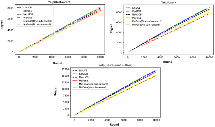
As the sub-rewards are not always available in many cases, in this subsection, we evaluate MuFasa with partially available sub-rewards on Yelp and Mnist+NotMnist data sets. Therefore, we build another two variants of MuFasa: (1) MuFasa (One sub-reward) is provided with the final reward and one sub-reward of the first bandit; (2) MuFasa (No sub-reward) does not receive any sub-rewards except the final reward. Here, we use the $H_{1}$ as the final reward function.

Figure 5 and Figure 6 show the regret comparison with the two variants of MuFasa, where MuFasa exhibits the robustness with respect to the lack of sub-rewards. Indeed, the sub-reward can provide more information to learn, while MuFasa (One sub-reward) still outperforms all the baselines, because the final reward enables MuFasa to learn the all bandits jointly and the sub-reward strengthens the capacity of learning the exclusive features of each bandit. In contrast, all the baselines treat each bandit separately. Without any-rewards, MuFasa still achieves the acceptable performance. On the Yelp data set, the regret of MuFasa (No sub-reward) is still lower than the best baseline NeuUCB while lacking considerable information. On the Mnist+NotMnist data set, although MuFasa (No sub-reward) does not outperform the baselines, its performance is still closed to NeuUCB. Therefore, as long as the final reward is provided, MuFasa can tackle the multi-facet problem effectively. Moreover, MuFasa can leverage available sub-rewards to improve the performance.

7. Conclusion

In this paper, we define and study the novel problem of the multi-facet contextual bandits, motivated by real applications such as comprehensive personalized recommendation and healthcare. We propose a new bandit algorithm, MuFasa. It utilizes the neural networks to learn the reward functions of multiple bandits jointly and explores new information by a comprehensive upper confidence bound. Moreover, we prove that MuFasa can achieve the $\widetilde{\mathcal{O}}((K+1)\sqrt{T})$ regret bound under mild assumptions. Finally, we conduct extensive experiments to show the effectiveness of MuFasa on personalized recommendation and classification tasks, as well as the robustness of MuFasa in the lack of sub-rewards.

Acknowledgement

This work is supported by National Science Foundation under Award No. IIS-1947203 and IIS-2002540, and the U.S. Department of Homeland Security under Grant Award Number 17STQAC00001-03-03. The views and conclusions are those of the authors and should not be interpreted as representing the official policies of the funding agencies or the government.

References

(1)
Abbasi-Yadkori et al. (2011) Yasin Abbasi-Yadkori, Dávid Pál, and Csaba Szepesvári. 2011. Improved algorithms for linear stochastic bandits. In Advances in Neural Information Processing Systems. 2312–2320.
Agrawal and Goyal (2013) Shipra Agrawal and Navin Goyal. 2013. Thompson sampling for contextual bandits with linear payoffs. In International Conference on Machine Learning. PMLR, 127–135.
Allen-Zhu et al. (2019) Zeyuan Allen-Zhu, Yuanzhi Li, and Zhao Song. 2019. A convergence theory for deep learning via over-parameterization. In International Conference on Machine Learning. PMLR, 242–252.
Allesiardo et al. (2014) Robin Allesiardo, Raphaël Féraud, and Djallel Bouneffouf. 2014. A neural networks committee for the contextual bandit problem. In International Conference on Neural Information Processing. Springer, 374–381.
Arora et al. (2019) Sanjeev Arora, Simon S Du, Wei Hu, Zhiyuan Li, Russ R Salakhutdinov, and Ruosong Wang. 2019. On exact computation with an infinitely wide neural net. In Advances in Neural Information Processing Systems. 8141–8150.
Audibert and Bubeck (2010) Jean-Yves Audibert and Sébastien Bubeck. 2010. Best arm identification in multi-armed bandits. In Conference on Learning Theory (COLT). 41–53.
Auer et al. (2002a) Peter Auer, Nicolo Cesa-Bianchi, and Paul Fischer. 2002a. Finite-time analysis of the multiarmed bandit problem. Machine learning 47, 2-3 (2002), 235–256.
Auer et al. (2002b) Peter Auer, Nicolo Cesa-Bianchi, Yoav Freund, and Robert E Schapire. 2002b. The nonstochastic multiarmed bandit problem. SIAM journal on computing 32, 1 (2002), 48–77.
Azizzadenesheli et al. (2018) Kamyar Azizzadenesheli, Emma Brunskill, and Animashree Anandkumar. 2018. Efficient exploration through bayesian deep q-networks. In 2018 Information Theory and Applications Workshop (ITA). IEEE, 1–9.
Ban and He (2020) Yikun Ban and Jingrui He. 2020. Generic Outlier Detection in Multi-Armed Bandit. In Proceedings of the 26th ACM SIGKDD International Conference on Knowledge Discovery & Data Mining. 913–923.
Ban and He (2021) Yikun Ban and Jingrui He. 2021. Local Clustering in Contextual Multi-Armed Bandits. arXiv preprint arXiv:2103.00063 (2021).
Bastani and Bayati (2020) Hamsa Bastani and Mohsen Bayati. 2020. Online decision making with high-dimensional covariates. Operations Research 68, 1 (2020), 276–294.
Bubeck et al. (2011) Sébastien Bubeck, Rémi Munos, Gilles Stoltz, and Csaba Szepesvári. 2011. X-Armed Bandits. Journal of Machine Learning Research 12, 5 (2011).
Buccapatnam et al. (2013) Swapna Buccapatnam, Atilla Eryilmaz, and Ness B Shroff. 2013. Multi-armed bandits in the presence of side observations in social networks. In 52nd IEEE Conference on Decision and Control. IEEE, 7309–7314.
Cao and Gu (2019) Yuan Cao and Quanquan Gu. 2019. Generalization bounds of stochastic gradient descent for wide and deep neural networks. In Advances in Neural Information Processing Systems. 10836–10846.
Chen et al. (2013) Wei Chen, Yajun Wang, and Yang Yuan. 2013. Combinatorial multi-armed bandit: General framework and applications. In International Conference on Machine Learning. PMLR, 151–159.
Chen et al. (2016) Wei Chen, Yajun Wang, Yang Yuan, and Qinshi Wang. 2016. Combinatorial multi-armed bandit and its extension to probabilistically triggered arms. The Journal of Machine Learning Research 17, 1 (2016), 1746–1778.
Deshmukh et al. (2017) Aniket Anand Deshmukh, Urun Dogan, and Clay Scott. 2017. Multi-task learning for contextual bandits. In Advances in neural information processing systems. 4848–4856.
Dimakopoulou et al. (2019) Maria Dimakopoulou, Zhengyuan Zhou, Susan Athey, and Guido Imbens. 2019. Balanced linear contextual bandits. In Proceedings of the AAAI Conference on Artificial Intelligence, Vol. 33. 3445–3453.
Durand et al. (2018) Audrey Durand, Charis Achilleos, Demetris Iacovides, Katerina Strati, Georgios D Mitsis, and Joelle Pineau. 2018. Contextual bandits for adapting treatment in a mouse model of de novo carcinogenesis. In Machine Learning for Healthcare Conference. 67–82.
Fu et al. (2020) Dongqi Fu, Zhe Xu, Bo Li, Hanghang Tong, and Jingrui He. 2020. A View-Adversarial Framework for Multi-View Network Embedding. In Proceedings of the 29th ACM International Conference on Information & Knowledge Management. 2025–2028.
Gentile et al. (2017) Claudio Gentile, Shuai Li, Purushottam Kar, Alexandros Karatzoglou, Giovanni Zappella, and Evans Etrue. 2017. On context-dependent clustering of bandits. In Proceedings of the 34th International Conference on Machine Learning-Volume 70. JMLR. org, 1253–1262.
Gentile et al. (2014) Claudio Gentile, Shuai Li, and Giovanni Zappella. 2014. Online clustering of bandits. In International Conference on Machine Learning. 757–765.
Jacot et al. (2018) Arthur Jacot, Franck Gabriel, and Clément Hongler. 2018. Neural tangent kernel: Convergence and generalization in neural networks. In Advances in neural information processing systems. 8571–8580.
Jing et al. (2021) Baoyu Jing, Chanyoung Park, and Hanghang Tong. 2021. HDMI: High-order Deep Multiplex Infomax. arXiv preprint arXiv:2102.07810 (2021).
Langford and Zhang (2008) John Langford and Tong Zhang. 2008. The epoch-greedy algorithm for multi-armed bandits with side information. In Advances in neural information processing systems. 817–824.
LeCun et al. (1998) Yann LeCun, Léon Bottou, Yoshua Bengio, and Patrick Haffner. 1998. Gradient-based learning applied to document recognition. Proc. IEEE 86, 11 (1998), 2278–2324.
Li et al. (2010) Lihong Li, Wei Chu, John Langford, and Robert E Schapire. 2010. A contextual-bandit approach to personalized news article recommendation. In Proceedings of the 19th international conference on World wide web. 661–670.
Li et al. (2016a) Shuai Li, Alexandros Karatzoglou, and Claudio Gentile. 2016a. Collaborative filtering bandits. In Proceedings of the 39th International ACM SIGIR conference on Research and Development in Information Retrieval. 539–548.
Li et al. (2016b) Shuai Li, Baoxiang Wang, Shengyu Zhang, and Wei Chen. 2016b. Contextual combinatorial cascading bandits. In International conference on machine learning. PMLR, 1245–1253.
Lipton et al. (2018) Zachary Lipton, Xiujun Li, Jianfeng Gao, Lihong Li, Faisal Ahmed, and Li Deng. 2018. Bbq-networks: Efficient exploration in deep reinforcement learning for task-oriented dialogue systems. In Proceedings of the AAAI Conference on Artificial Intelligence, Vol. 32.
Liu et al. (2011) Haoyang Liu, Keqin Liu, and Qing Zhao. 2011. Logarithmic weak regret of non-bayesian restless multi-armed bandit. In 2011 IEEE International Conference on Acoustics, Speech and Signal Processing (ICASSP). IEEE, 1968–1971.
Qin et al. (2014) Lijing Qin, Shouyuan Chen, and Xiaoyan Zhu. 2014. Contextual combinatorial bandit and its application on diversified online recommendation. In Proceedings of the 2014 SIAM International Conference on Data Mining. SIAM, 461–469.
Riquelme et al. (2018) Carlos Riquelme, George Tucker, and Jasper Snoek. 2018. Deep bayesian bandits showdown: An empirical comparison of bayesian deep networks for thompson sampling. arXiv preprint arXiv:1802.09127 (2018).
Roweis and Saul (2000) Sam T Roweis and Lawrence K Saul. 2000. Nonlinear dimensionality reduction by locally linear embedding. science 290, 5500 (2000), 2323–2326.
Srinivas et al. (2009) Niranjan Srinivas, Andreas Krause, Sham M Kakade, and Matthias Seeger. 2009. Gaussian process optimization in the bandit setting: No regret and experimental design. arXiv preprint arXiv:0912.3995 (2009).
Su and Khoshgoftaar (2009) Xiaoyuan Su and Taghi M Khoshgoftaar. 2009. A survey of collaborative filtering techniques. Advances in artificial intelligence 2009 (2009).
Thompson (1933) William R Thompson. 1933. On the likelihood that one unknown probability exceeds another in view of the evidence of two samples. Biometrika 25, 3/4 (1933), 285–294.
Valko et al. (2013) Michal Valko, Nathaniel Korda, Rémi Munos, Ilias Flaounas, and Nelo Cristianini. 2013. Finite-time analysis of kernelised contextual bandits. arXiv preprint arXiv:1309.6869 (2013).
Wu et al. (2016) Qingyun Wu, Huazheng Wang, Quanquan Gu, and Hongning Wang. 2016. Contextual bandits in a collaborative environment. In Proceedings of the 39th International ACM SIGIR conference on Research and Development in Information Retrieval. 529–538.
Yang and Wang (2020) Lin Yang and Mengdi Wang. 2020. Reinforcement learning in feature space: Matrix bandit, kernels, and regret bound. In International Conference on Machine Learning. PMLR, 10746–10756.
Zahavy and Mannor (2019) Tom Zahavy and Shie Mannor. 2019. Deep neural linear bandits: Overcoming catastrophic forgetting through likelihood matching. arXiv preprint arXiv:1901.08612 (2019).
Zheng et al. (2021) Lecheng Zheng, Yu Cheng, Hongxia Yang, Nan Cao, and Jingrui He. 2021. Deep Co-Attention Network for Multi-View Subspace Learning. arXiv preprint arXiv:2102.07751 (2021).
Zhou et al. (2015) Dawei Zhou, Jingrui He, K Selçuk Candan, and Hasan Davulcu. 2015. MUVIR: Multi-View Rare Category Detection.. In IJCAI. Citeseer, 4098–4104.
Zhou et al. (2020a) Dongruo Zhou, Lihong Li, and Quanquan Gu. 2020a. Neural contextual bandits with UCB-based exploration. In International Conference on Machine Learning. PMLR, 11492–11502.
Zhou et al. (2020c) Dawei Zhou, Lecheng Zheng, Yada Zhu, Jianbo Li, and Jingrui He. 2020c. Domain adaptive multi-modality neural attention network for financial forecasting. In Proceedings of The Web Conference 2020. 2230–2240.
Zhou et al. (2020b) Yao Zhou, Jianpeng Xu, Jun Wu, Zeinab Taghavi Nasrabadi, Evren Korpeoglu, Kannan Achan, and Jingrui He. 2020b. GAN-based Recommendation with Positive-Unlabeled Sampling. arXiv preprint arXiv:2012.06901 (2020).

8. appendix

Definition 8.1.

Given the context vectors $\{\mathbf{x}_{t}\}_{t=1}^{T}$ and the rewards $\{r_{t}\}_{t=1}^{T}$ , then we define the estimation $\bm{\theta}^{\prime}$ via ridge regression:

		$\displaystyle\mathbf{A}_{t}^{\prime}=\lambda\mathbf{I}+\sum_{i=1}^{t}g(\mathbf{x}_{t};\bm{\theta}_{0})g(\mathbf{x}_{t};\bm{\theta}_{0})^{\intercal}/m$
		$\displaystyle\mathbf{b}_{t}^{\prime}=\sum_{i=1}^{t}r_{t}g(\mathbf{x}_{t};\bm{\theta}_{0})/\sqrt{m}$
		$\displaystyle\bm{\theta}^{\prime}=\mathbf{A}^{-1}_{t}\mathbf{b}_{t}$
		$\displaystyle\mathbf{A}_{t}=\lambda\mathbf{I}+\sum_{i=1}^{t}g(\mathbf{x}_{t};\bm{\theta}_{t})g(\mathbf{x}_{t};\bm{\theta}_{t})^{\intercal}/m$

Definition 8.2 ( NTK (Jacot et al., 2018; Cao and Gu, 2019)).

Let $\mathcal{N}$ denote the normal distribution. Define

		$\displaystyle\mathbf{M}_{i,j}^{0}=\bm{\Sigma}^{0}_{i,j}=\langle\mathbf{x}_{i},\mathbf{x}_{j}\rangle,\ \ \mathbf{N}^{l}_{i,j}=\begin{pmatrix}\bm{\Sigma}^{l}_{i,i}&\bm{\Sigma}^{l}_{i,j}\\ \bm{\Sigma}^{l}_{j,i}&\bm{\Sigma}^{l}_{j,j}\end{pmatrix}$
		$\displaystyle\bm{\Sigma}^{l}_{i,j}=2\mathbb{E}_{a,b\sim\mathcal{N}(\mathbf{0},\mathbf{N}_{i,j}^{l-1})}[\sigma(a)\sigma(b)]$
		$\displaystyle\mathbf{M}_{i,j}^{l}=2\mathbf{M}_{i,j}^{l-1}\mathbb{E}_{a,b\sim\mathcal{N}(\mathbf{0},\mathbf{N}_{i,j}^{l-1})}[\sigma^{\prime}(a)\sigma^{\prime}(b)]+\bm{\Sigma}^{l}_{i,j}.$

Then, given the contexts $\{\mathbf{x}_{t}\}_{t=1}^{T}$ , the Neural Tangent Kernel is defined as $\mathbf{M}=(\mathbf{M}^{L}+\bm{\Sigma}^{L})/2$ .

Definition 8.3 (Effective Dimension (Zhou et al., 2020a)).

Given the contexts $\{\mathbf{x}_{t}\}_{t=1}^{T}$ , the effective dimension $\widetilde{P}$ is defined as

\widetilde{P}=\frac{\log\text{det}(\mathbf{I}+\mathbf{M}/\lambda)}{\log(1+T/\lambda)}.

Proof of Lemma 5.2. Given a set of context vectors $\{\mathbf{x}\}_{t=1}^{T}$ with the ground-truth function $h$ and a fully-connected neural network $f$ , we have

		$\displaystyle\left\|h(\mathbf{x}_{t})-f(\mathbf{x}_{t};\bm{\theta}_{t})\right\|$
	$\displaystyle\leq$	$\displaystyle\left\|h(\mathbf{x}_{t})-\langle g(\mathbf{x}_{t};\bm{\theta}_{0}),\bm{\theta}^{\prime}/\sqrt{m}\rangle\right\|+\left\|f(\mathbf{x}_{t};\bm{\theta}_{t})-\langle g(\mathbf{x}_{t};\bm{\theta}_{0}),\bm{\theta}^{\prime}/\sqrt{m}\rangle\right\|$

where $\bm{\theta}^{\prime}$ is the estimation of ridge regression from Definition 8.1. Then, based on the Lemma 5.1, there exists $\bm{\theta}^{\ast}\in\mathbf{R}^{P}$ such that $h(\mathbf{x}_{t})=\left\langle g(\mathbf{x}_{i},\bm{\theta}_{0}),\bm{\theta}^{\ast}\right\rangle$ . Thus, we have

		$\displaystyle\ \ \left\|h(\mathbf{x}_{t})-\langle g(\mathbf{x}_{t};\bm{\theta}_{0}),\bm{\theta}^{\prime}/\sqrt{m}\rangle\right\|$
		$\displaystyle=\left\|\left\langle g(\mathbf{x}_{i},\bm{\theta}_{0})/\sqrt{m},\sqrt{m}\bm{\theta}^{\ast}\right\rangle-\left\langle g(\mathbf{x}_{i},\bm{\theta}_{0})/\sqrt{m},\bm{\theta}^{\prime}\right\rangle\right\|\leq$
		$\displaystyle\left(\sqrt{\log\left(\frac{\text{det}(\mathbf{A}_{t}^{\prime})}{\text{det}(\lambda\mathbf{I})}\right)-2\log\delta}+\lambda^{1/2}S\right)\\|g(\mathbf{x}_{t};\bm{\theta}_{0})/\sqrt{m}\\|_{\mathbf{A}_{t}^{{}^{\prime}-1}}$

where the final inequality is based on the the Theorem 2 in (Abbasi-Yadkori et al., 2011), with probability at least $1-\delta$ , for any $t\in[T]$ .

Second we need to bound

		$\displaystyle\left\|f(\mathbf{x}_{t};\bm{\theta}_{t})-\langle g(\mathbf{x}_{t};\bm{\theta}_{0}),\bm{\theta}^{\prime}/\sqrt{m}\rangle\right\|$
	$\displaystyle\leq$	$\displaystyle\left\|f(\mathbf{x}_{t};\bm{\theta}_{t})-\langle g(\mathbf{x}_{t};\bm{\theta}_{0}),\bm{\theta}_{t}-\bm{\theta}_{0}\rangle\right\|$
		$\displaystyle+\left\|\langle g(\mathbf{x}_{t};\bm{\theta}_{0}),\bm{\theta}_{t}-\bm{\theta}_{0}\rangle-\langle g(\mathbf{x}_{t};\bm{\theta}_{0}),\bm{\theta}^{\prime}/\sqrt{m}\rangle\right\|$

To bound the above inequality, we first bound

		$\displaystyle\left\|f(\mathbf{x}_{t};\bm{\theta}_{t})-\langle g(\mathbf{x}_{t};\bm{\theta}_{0}),\bm{\theta}_{t}-\bm{\theta}_{0}\rangle\right\|$
	$\displaystyle=$	$\displaystyle\left\|f(\mathbf{x}_{t};\bm{\theta}_{t})-f(\mathbf{x}_{t};\bm{\theta}_{0})-\langle g(\mathbf{x}_{t};\bm{\theta}_{0}),\bm{\theta}_{t}-\bm{\theta}_{0}\rangle\right\|$
	$\displaystyle\leq$	$\displaystyle C_{2}\tau^{4/3}L^{3}\sqrt{m\log m}\leq C_{2}m^{-1/6}\sqrt{\log m}t^{2/3}\lambda^{-2/3}L^{3}.$

where $f(\mathbf{x}_{t};\bm{\theta}_{0})=0$ due to the random initialization of $\bm{\theta}_{0}$ . The first inequality is derived by Lemma 8.5. According to the Lemma 8.7, it has $\|\bm{\theta}_{t}-\bm{\theta}_{0}\|_{2}\leq 2\sqrt{\frac{t}{m\lambda}}$ . Then, replacing $\tau$ by $2\sqrt{\frac{t}{m\lambda}}$ , we obtain the second inequality.

Next, we need to bound

		$\displaystyle\|\langle g(\mathbf{x}_{t};\bm{\theta}_{0}),\bm{\theta}_{t}-\bm{\theta}_{0}\rangle-\langle g(\mathbf{x}_{t};\bm{\theta}_{0}),\bm{\theta}^{\prime}/\sqrt{m}\rangle\|$
	$\displaystyle=$	$\displaystyle\|\langle g(\mathbf{x}_{t};\bm{\theta}_{0})/\sqrt{m},\sqrt{m}(\bm{\theta}_{t}-\bm{\theta}_{0}-\bm{\theta}^{\prime}/\sqrt{m})\rangle\|$
	$\displaystyle\leq$	$\displaystyle\\|g(\mathbf{x}_{t};\bm{\theta}_{0})/\sqrt{m}\\|_{\mathbf{A}_{t}^{-1}}\cdot\sqrt{m}\\|\bm{\theta}_{t}-\bm{\theta}_{0}-\bm{\theta}^{\prime}/\sqrt{m}\\|_{\mathbf{A}_{t}}$
	$\displaystyle\leq$	$\displaystyle\\|g(\mathbf{x}_{t};\bm{\theta}_{0})/\sqrt{m}\\|_{\mathbf{A}_{t}^{-1}}\cdot\sqrt{m}\\|{\mathbf{A}_{t}}\\|_{2}\cdot\\|\bm{\theta}_{t}-\bm{\theta}_{0}-\bm{\theta}^{\prime}/\sqrt{m}\\|_{2}.$

Due to the Lemma 8.6 and Lemma 8.7, we have

		$\displaystyle\sqrt{m}\\|{\mathbf{A}_{t}}\\|_{2}\cdot\\|\bm{\theta}_{t}-\bm{\theta}_{0}-\bm{\theta}^{\prime}/\sqrt{m}\\|_{2}\leq\sqrt{m}(\lambda+t\mathcal{O}(L))$
		$\displaystyle\cdot\left((1-\eta m\lambda)^{J/2}\sqrt{t/(m\lambda)}+C_{4}m^{-2/3}\sqrt{\log m}L^{7/2}t^{5/3}\lambda^{-5/3}(1+\sqrt{t/\lambda})\right)$
		$\displaystyle\leq(\lambda+t\mathcal{O}(L))$
		$\displaystyle\cdot((1-\eta m\lambda)^{J/2}\sqrt{t/\lambda}+C_{4}m^{-1/6}\sqrt{\log m}L^{7/2}t^{5/3}\lambda^{-5/3}(1+\sqrt{t/\lambda}))$
		$\displaystyle\leq(\lambda+t\mathcal{O}(L))\cdot((1-\eta m\lambda)^{J/2}\sqrt{t/\lambda})+1$

where the last inequality is because $m$ is sufficiently large. Therefore, we have

		$\displaystyle\left\|f(\mathbf{x}_{t};\bm{\theta}_{t})-\langle g(\mathbf{x}_{t};\bm{\theta}_{0}),\bm{\theta}^{\prime}/\sqrt{m}\rangle\right\|$
	$\displaystyle\leq$	$\displaystyle\left((\lambda+t\mathcal{O}(L))\cdot((1-\eta m\lambda)^{J/2}\sqrt{t/\lambda})+1\right)\\|g(\mathbf{x}_{t};\bm{\theta}_{0})/\sqrt{m}\\|_{\mathbf{A}_{t}^{-1}}$
		$\displaystyle+C_{2}m^{-1/6}\sqrt{\log m}t^{2/3}\lambda^{-2/3}L^{3}$

And we have

		$\displaystyle\\|g(\mathbf{x}_{t};\bm{\theta}_{0})/\sqrt{m}\\|_{\mathbf{A}_{t}^{-1}}$
	$\displaystyle=$	$\displaystyle\\|g(\mathbf{x}_{t};\bm{\theta}_{t})+g(\mathbf{x}_{t};\bm{\theta}_{0})-g(\mathbf{x}_{t};\bm{\theta}_{t})\\|_{\mathbf{A}_{t}^{-1}}/\sqrt{m}$
	$\displaystyle\leq$	$\displaystyle\\|g(\mathbf{x}_{t};\bm{\theta}_{t})/\sqrt{m}\\|_{\mathbf{A}_{t}^{-1}}+\\|\mathbf{A}_{t}^{-1}\\|_{2}\\|g(\mathbf{x}_{t};\bm{\theta}_{0})-g(\mathbf{x}_{t};\bm{\theta}_{t})\\|_{2}/\sqrt{m}$
	$\displaystyle\leq$	$\displaystyle\\|g(\mathbf{x}_{t};\bm{\theta}_{t})/\sqrt{m}\\|_{\mathbf{A}_{t}^{-1}}+\lambda^{-1}m^{-1/6}\sqrt{\log m}t^{1/6}\lambda^{-1/6}L^{7/2}$

where the last inequality is because of Lemma 8.8 with Lemma 8.7 and $\|\mathbf{A}_{t}\|_{2}\geq\|\lambda\mathbf{I}\|_{2}$ .

Finally, putting everything together, we have

	$\displaystyle\left\|h(\mathbf{x}_{t})-f(\mathbf{x}_{t};\bm{\theta}_{t})\right\|$	$\displaystyle\leq\gamma_{1}\\|g(\mathbf{x}_{t};\bm{\theta}_{t})/\sqrt{m}\\|_{\mathbf{A}_{t}^{-1}}+\gamma_{2}\\|g(\mathbf{x}_{t};\bm{\theta}_{0})/\sqrt{m}\\|_{\mathbf{A}_{t}^{{}^{\prime}-1}}$
		$\displaystyle+\gamma_{1}\gamma_{3}+\gamma_{4}.$

Proof of Theorem 5.3. First, considering an individual bandit $k\in[K]$ with the set of context vectors $\{\mathbf{x}_{t}^{k}\}_{t=1}^{T}$ and the set of sub-rewards $\{r_{t}^{k}\}_{t=1}^{T}$ , we can build upper confidence bound of $f_{k}(\mathbf{x}_{t}^{k};\bm{\theta}^{k}_{t})$ with respect to $h_{k}(\mathbf{x}_{t}^{k})$ based on the Lemma 5.2. Denote the UCB by $\mathcal{B}(\mathbf{x}_{t}^{k},m,L_{1},\delta^{\prime})$ , with probability at least $1-\delta^{\prime}$ , for any $t\in[T]$ we have

|f_{k}(\mathbf{x}_{t}^{k};\bm{\theta}^{k}_{t})-h_{k}(\mathbf{x}_{t}^{k})|\leq\mathcal{B}(\mathbf{x}_{t}^{k},m,L_{1},\delta^{\prime},t)=\mathcal{B}^{k}.

Next, apply the union bound on the $K+1$ networks, we have $\delta^{\prime}=\delta/(K+1)$ in each round $t$ .

Next we need to bound

		$\displaystyle\left\|H\left(\text{vec}(\mathbf{r}_{t})\right)-H\left(\mathbf{f}_{t}\right)\right\|$
	$\displaystyle\leq$	$\displaystyle\bar{C}\sqrt{\sum_{k=1}^{K}\|f_{k}(\mathbf{x}_{t}^{k};\bm{\theta}^{k}_{t})-h_{k}(\mathbf{x}_{t}^{k})\|^{2}}$
	$\displaystyle\leq$	$\displaystyle\bar{C}\sqrt{\sum_{k=1}^{K}(\mathcal{B}^{k})^{2}}\leq\bar{C}\sum_{k=1}^{K}\mathcal{B}^{k}$

where the first inequality is because $H$ is a $\bar{C}$ -lipschitz continuous function. Therefore, we have

		$\displaystyle\|\mathcal{F}(\mathbf{X}_{t})-\mathcal{H}(\mathbf{X}_{t})\|=\|F(\mathbf{f}_{t};\bm{\theta}^{\Sigma})-H(\text{vec}(\mathbf{r}_{t}))\|$
	$\displaystyle\leq$	$\displaystyle\left\|F(\mathbf{f}_{t};\bm{\theta}^{\Sigma})-H\left(\mathbf{f}_{t}\right)\right\|+\left\|H\left(\mathbf{f}_{t}\right)-H(\text{vec}(\mathbf{r}_{t}))\right\|\leq\bar{C}\sum_{k=1}^{K}\mathcal{B}^{k}+\mathcal{B}^{F}.$

This completes the proof of the claim.

Lemma 8.4.

With probability at least $1-\delta^{\prime}$ , we have

	$\displaystyle(1)\\|\mathbf{A}_{t}\\|_{2},\\|\mathbf{A}_{t}^{\prime}\\|_{2}$	$\displaystyle\leq\lambda+t\mathcal{O}(L)$
	$\displaystyle(2)\log\frac{\text{det}(\mathbf{A}_{t}^{\prime})}{\text{det}(\lambda\mathbf{I})}$	$\displaystyle\leq\widetilde{P}\log(1+T/\lambda)+1/\lambda$
	$\displaystyle(3)\|\log\frac{\text{det}(\mathbf{A}_{t})}{\text{det}(\lambda\mathbf{I})}-\log\frac{\text{det}(\mathbf{A}_{t}^{\prime})}{\text{det}(\lambda\mathbf{I})}\|$	$\displaystyle\leq\mathcal{O}(m^{-1/6}\sqrt{\log m}L^{4}t^{5/3}\lambda^{-1/6}).$

where $(3)$ is referred from Lemma B.3 in (Zhou et al., 2020a).

Proof of Lemma 8.4. For (1), based on the Lemma 8.6, for any $\mathbf{x}_{t}\in\{\mathbf{x}_{i}\}_{i=1}^{T}$ ,
$\|g(\mathbf{x}_{t};\bm{\theta}_{0})\|_{F}\leq\mathcal{O}(\sqrt{mL})$ . Then, for the first item:

		$\displaystyle\\|\mathbf{A}_{t}\\|_{2}=\\|\lambda\mathbf{I}+\sum_{i=1}^{t}g(\mathbf{x}_{i};\bm{\theta}_{t})g(\mathbf{x}_{i};\bm{\theta}_{t})^{\intercal}/m\\|_{2}$
		$\displaystyle\leq\\|\lambda\mathbf{I}\\|_{2}+\\|\sum_{i=1}^{t}g(\mathbf{x}_{i};\bm{\theta}_{t})g(\mathbf{x}_{i};\bm{\theta}_{t})^{\intercal}/m\\|_{2}$
		$\displaystyle\leq\lambda+\sum_{i=1}^{t}\\|g(\mathbf{x}_{i};\bm{\theta}_{t})\\|_{2}^{2}/m\leq\lambda+\sum_{i=1}^{t}\\|g(\mathbf{x}_{i};\bm{\theta}_{t})\\|_{F}^{2}/m$
		$\displaystyle\leq\lambda+t\mathcal{O}(L).$

Same proof workflow for $\|\mathbf{A}_{t}^{\prime}\|_{2}$ . For (2), we have

	$\displaystyle\log\frac{\text{det}(\mathbf{A}_{t}^{\prime})}{\text{det}(\lambda\mathbf{I})}$	$\displaystyle=\log\text{det}(\mathbf{I}+\sum_{t=1}^{T}g(\mathbf{x}_{t};\bm{\theta}_{0})g(\mathbf{x}_{t};\bm{\theta}_{0})^{\intercal}/(m\lambda))$
		$\displaystyle=\text{det}(\mathbf{I}+\mathbf{G}\mathbf{G}^{\intercal}/\lambda)$

where $\mathbf{G}=(g(\mathbf{x}_{1};\bm{\theta}_{0}),\dots,g(\mathbf{x}_{T};\bm{\theta}_{0}))/\sqrt{m}$ .

According to the Theorem 3.1 in (Arora et al., 2019), when $m=\Omega(\frac{L^{6}\log{L/\delta}}{\epsilon^{4}})$ , with probability at least $1-\delta$ , for any $\mathbf{x}_{i},\mathbf{x}_{j}\in\{\mathbf{x}_{t}\}_{t=1}^{T}$ , it has

|g(\mathbf{x}_{i};\bm{\theta}_{0})^{\intercal}g(\mathbf{x}_{j};\bm{\theta}_{0})/m-\mathbf{M}_{i,j}|\leq\epsilon.

Therefore, we have

	$\displaystyle\\|\mathbf{G}\mathbf{G}^{\intercal}-\mathbf{M}\\|_{F}$	$\displaystyle=\sqrt{\sum_{i=1}^{T}\sum_{j=1}^{T}\|g(\mathbf{x}_{i};\bm{\theta}_{0})^{\intercal}g(\mathbf{x}_{j};\bm{\theta}_{0})/m-\mathbf{M}_{i,j}\|^{2}}$
		$\displaystyle\leq T\epsilon.$

Then, we have

		$\displaystyle\log\det(\mathbf{I}+\mathbf{G}\mathbf{G}^{\intercal}/\lambda)$
		$\displaystyle=\log\text{det}(\mathbf{I}+\mathbf{M}\lambda+(\mathbf{G}\mathbf{G}^{\intercal}-\mathbf{M})/\lambda)$
		$\displaystyle\leq\log\text{det}(\mathbf{I}+\mathbf{M}\lambda)+\langle(\mathbf{I}+\mathbf{M}\lambda)^{-1},(\mathbf{G}\mathbf{G}^{\intercal}-\mathbf{M})/\lambda\rangle$
		$\displaystyle\leq\log\text{det}(\mathbf{I}+\mathbf{M}\lambda)+\\|(\mathbf{I}+\mathbf{M}\lambda)^{-1}\\|_{F}\\|\mathbf{G}\mathbf{G}^{\intercal}-\mathbf{M}\\|_{F}/\lambda$
		$\displaystyle\leq\log\text{det}(\mathbf{I}+\mathbf{M}\lambda)+\sqrt{T}\\|\mathbf{G}\mathbf{G}^{\intercal}-\mathbf{M}\\|_{F}/\lambda$
		$\displaystyle\leq\log\text{det}(\mathbf{I}+\mathbf{M}\lambda)+\lambda^{-1}$
		$\displaystyle=\widetilde{P}\log(1+T/\lambda)+\lambda^{-1}.$

The first inequality is because the concavity of $\log\text{det}$ ; The third inequality is due to $\|(\mathbf{I}+\mathbf{M}\lambda)^{-1}\|_{F}\leq\|\mathbf{I}^{-1}\|_{F}\leq\sqrt{T}$ ; The last inequality is because of the choice the $m$ ; The last equality is because of the Definition 8.3.

Lemma 8.5 ( Lemma 4.1 in (Cao and Gu, 2019) ).

There exist constants $\{\bar{C}_{i=1}^{3}\}\geq 0$ such that for any $\delta\geq 0$ , if $\tau$ satisfies that

\tau\leq\bar{C}_{2}L^{-6}[\log m]^{-3/2},

then with probability at least $1-\delta$ , for all $\bm{\theta}^{1},\bm{\theta}^{2}$ satisfying $\|\bm{\theta}^{1}-\bm{\theta}_{0}\|\leq\tau,\|\bm{\theta}^{2}-\bm{\theta}_{0}\|\leq\tau$ and for any $\mathbf{x}_{t}\in\{\mathbf{x}_{t}\}_{t=1}^{T}$ , we have

|f(\mathbf{x};\bm{\theta}^{1})-f(\mathbf{x};\bm{\theta}^{2})-\langle(g(\mathbf{x};\bm{\theta}^{2}),\bm{\theta}^{1}-\bm{\theta}^{2})\rangle|\leq\bar{C}_{3}\tau^{4/3}L^{3}\sqrt{m\log m}.

Lemma 8.6 (Lemma B.3 in (Cao and Gu, 2019) ).

There exist constants $\{C_{i}\}_{i=1}^{2}$ such that for any $\delta>0$ , if $\tau$ satisfies that

\tau\leq C_{1}L^{-6}(\log m)^{-3/2},

then, with probability at least $1-\delta$ , for any $\|\bm{\theta}-\bm{\theta}_{0}\|\leq\tau$ and $\mathbf{x}_{t}\in\{\mathbf{x}_{t}\}_{t=1}^{T}$ we have $\|g(\mathbf{x}_{t};\bm{\theta})\|_{2}\leq C_{2}\sqrt{mL}$ .

Lemma 8.7 (Lemma B.2 in (Zhou et al., 2020a) ).

For the $L$ -layer full-connected network $f$ , there exist constants $\{C_{i}\}_{i=1}^{5}\geq 0$ such that for $\delta>0$ , if for all $t\in[T]$ , $\eta,m$ satisfy

		$\displaystyle 2\sqrt{t/(m\lambda)}\geq C_{1}m^{-3/2}L^{-3/2}[\log(TL^{2}/\delta)]^{3/2},$
		$\displaystyle 2\sqrt{t/(m\lambda)}\leq C_{2}\min\{L^{-6}[\log m]^{-3/2},(m(\lambda\eta)^{2}L^{-6}t^{-1}(\log m)^{-1})^{3/8}\},$
		$\displaystyle\eta\leq C_{3}(m\lambda+tmL)^{-1},$
		$\displaystyle m^{1/6}\geq C_{4}\sqrt{\log m}L^{7/2}t^{7/6}\lambda^{-7/6}(1+\sqrt{t/\lambda}),$

then, with probability at least $1-\delta$ , it has

		$\displaystyle\\|\bm{\theta}_{t}-\bm{\theta}_{0}\\|\leq 2\sqrt{t/(m\lambda)}$
		$\displaystyle\\|\bm{\theta}_{t}-\bm{\theta}_{0}-\bm{\theta}^{\prime}\\|\leq$
		$\displaystyle(1-\eta m\lambda)^{J/2}\sqrt{t/(m\lambda)}+C_{5}m^{-2/3}\sqrt{\log m}L^{7/2}t^{5/3}\lambda^{-5/3}(1+\sqrt{t/\lambda}).$

Lemma 8.8 (Theorem 5 in (Allen-Zhu et al., 2019)).

With probability at least $1-\delta$ , there exist constants $C_{1},C_{2}$ such that if $\tau\leq C_{1}L^{-9/2}\log^{-3}m$ , for $\|\bm{\theta}_{t}-\bm{\theta}_{0}\|_{2}\leq\tau$ , we have

\|g(\mathbf{x}_{t};\bm{\theta}_{t})-g(\mathbf{x}_{t};\bm{\theta}_{0})\|_{2}\leq C_{2}\sqrt{\log m}\tau^{1/3}L^{3}\|g(\mathbf{x}_{t};\bm{\theta}_{0})\|_{2}.

8.1. Empirical Setting of UCB

UCB is the key component of MuFasa, determining the empirical performance. $UCB(\mathbf{X}_{t})$ (Lemma 5.2) can be formulated as

UCB(\mathbf{X}_{t})=(1-\lambda)\|g(\mathbf{x};\bm{\theta}_{t})\|_{\mathbf{A}_{t}^{-1}}+\lambda\|g(\mathbf{x};\bm{\theta}_{0})\|_{\mathbf{A}_{t}^{{}^{\prime}-1}}

where $g(\mathbf{x};\bm{\theta}_{0})$ is the gradient at initialization, $g(\mathbf{x};\bm{\theta}_{t})$ is the gradient after $k$ iterations of gradient descent, and $\lambda$ is a tunable parameter to trade off between them. Intuitively, $g(\mathbf{x};\bm{\theta}_{0})$ has more bias as the weights of neural network function $f$ are randomness initialized, which brings more exploration portion in decision making of each round. In contrast, $g(\mathbf{x};\bm{\theta}_{t})$ has more variance as the weights should be nearer to the optimum after gradient descent.

In the setting where the set of arms are fixed, given an arm $\mathbf{x}_{i}$ , let $m_{i}$ be the number of rounds that $\mathbf{x}_{i}$ has been played before. When $m_{i}$ is small, the learner should explore $\mathbf{x}_{i}$ more ( $\lambda$ is expected to be large). Instead, when $m_{i}$ is large, the leaner does not need more exploration on it. Therefore, $\lambda$ can be defined as a decreasing function with respect to $m_{i}$ , such as $\frac{1}{\sqrt{m_{i}+1}}$ and $\frac{1}{\log(m_{i}+1)}$ . In the setting without this condition, we can set $\lambda$ as a decreasing function with respect to the number of rounds $t$ , such as $\frac{1}{\sqrt{t+1}}$ and $\frac{1}{\log(t+1)}$ .

8.2. Future Work

This paper introduces a novel bandit problem, multi-facet contextual bandits. Based on empirical experiments and theoretical analysis, at least three factors play important roles in multi-facet bandits: (1) As all bandits are serving the same user, mutual influence does exist among bandits. Thus, how to extract and harness the mutual influence among bandits is one future-work direction; (2) The weights of bandits usually determine the final reward, since each bandit has a different impact on the serving user. For example, in the diabetes case, the bandit for selecting medications should have a higher weight than the bandit for recommending diabetes articles; (3) Sub-rewards contain crucial information and thus exploiting sub-rewards matters in this problem.

To solve multi-facet bandit problem, we propose the algorithm, MuFasa. However, there are three limitations implicitly shown in this paper: (1) For leveraging the sub-rewards, we assume the $\bar{C}$ -lipschitz continuity of final reward function, while $\bar{C}$ is usually unknown; (2) In the selection criteria of MuFasa, it needs to select one arm with the highest score from all possible combinations $\mathbf{S}_{t}$ (Eq. (2) and Eq. (5)). However, the size of $\mathbf{S}_{t}$ grows exponentially with respect to the number of bandits $K$ . (3) MuFasa only uses fully-connected work to exploit rewards, while many more advanced neural network models exist such as CNN, residual net, self-attention, etc.

		$\displaystyle\left\|f(\mathbf{x}_{t};\bm{\theta}_{t})-\langle g(\mathbf{x}_{t};\bm{\theta}_{0}),\bm{\theta}^{\prime}/\sqrt{m}\rangle\right\|$
	$\displaystyle\leq$	$\displaystyle\left\|f(\mathbf{x}_{t};\bm{\theta}_{t})-\langle g(\mathbf{x}_{t};\bm{\theta}_{0}),\bm{\theta}_{t}-\bm{\theta}_{0}\rangle\right\|$
		$\displaystyle+\left\|\langle g(\mathbf{x}_{t};\bm{\theta}_{0}),\bm{\theta}_{t}-\bm{\theta}_{0}\rangle-\langle g(\mathbf{x}_{t};\bm{\theta}_{0}),\bm{\theta}^{\prime}/\sqrt{m}\rangle\right\|$

		$\displaystyle\|\langle g(\mathbf{x}_{t};\bm{\theta}_{0}),\bm{\theta}_{t}-\bm{\theta}_{0}\rangle-\langle g(\mathbf{x}_{t};\bm{\theta}_{0}),\bm{\theta}^{\prime}/\sqrt{m}\rangle\|$
	$\displaystyle=$	$\displaystyle\|\langle g(\mathbf{x}_{t};\bm{\theta}_{0})/\sqrt{m},\sqrt{m}(\bm{\theta}_{t}-\bm{\theta}_{0}-\bm{\theta}^{\prime}/\sqrt{m})\rangle\|$
	$\displaystyle\leq$	$\displaystyle\\|g(\mathbf{x}_{t};\bm{\theta}_{0})/\sqrt{m}\\|_{\mathbf{A}_{t}^{-1}}\cdot\sqrt{m}\\|\bm{\theta}_{t}-\bm{\theta}_{0}-\bm{\theta}^{\prime}/\sqrt{m}\\|_{\mathbf{A}_{t}}$
	$\displaystyle\leq$	$\displaystyle\\|g(\mathbf{x}_{t};\bm{\theta}_{0})/\sqrt{m}\\|_{\mathbf{A}_{t}^{-1}}\cdot\sqrt{m}\\|{\mathbf{A}_{t}}\\|_{2}\cdot\\|\bm{\theta}_{t}-\bm{\theta}_{0}-\bm{\theta}^{\prime}/\sqrt{m}\\|_{2}.$

		$\displaystyle\\|g(\mathbf{x}_{t};\bm{\theta}_{0})/\sqrt{m}\\|_{\mathbf{A}_{t}^{-1}}$
	$\displaystyle=$	$\displaystyle\\|g(\mathbf{x}_{t};\bm{\theta}_{t})+g(\mathbf{x}_{t};\bm{\theta}_{0})-g(\mathbf{x}_{t};\bm{\theta}_{t})\\|_{\mathbf{A}_{t}^{-1}}/\sqrt{m}$
	$\displaystyle\leq$	$\displaystyle\\|g(\mathbf{x}_{t};\bm{\theta}_{t})/\sqrt{m}\\|_{\mathbf{A}_{t}^{-1}}+\\|\mathbf{A}_{t}^{-1}\\|_{2}\\|g(\mathbf{x}_{t};\bm{\theta}_{0})-g(\mathbf{x}_{t};\bm{\theta}_{t})\\|_{2}/\sqrt{m}$
	$\displaystyle\leq$	$\displaystyle\\|g(\mathbf{x}_{t};\bm{\theta}_{t})/\sqrt{m}\\|_{\mathbf{A}_{t}^{-1}}+\lambda^{-1}m^{-1/6}\sqrt{\log m}t^{1/6}\lambda^{-1/6}L^{7/2}$

		$\displaystyle\\|\mathbf{A}_{t}\\|_{2}=\\|\lambda\mathbf{I}+\sum_{i=1}^{t}g(\mathbf{x}_{i};\bm{\theta}_{t})g(\mathbf{x}_{i};\bm{\theta}_{t})^{\intercal}/m\\|_{2}$
		$\displaystyle\leq\\|\lambda\mathbf{I}\\|_{2}+\\|\sum_{i=1}^{t}g(\mathbf{x}_{i};\bm{\theta}_{t})g(\mathbf{x}_{i};\bm{\theta}_{t})^{\intercal}/m\\|_{2}$
		$\displaystyle\leq\lambda+\sum_{i=1}^{t}\\|g(\mathbf{x}_{i};\bm{\theta}_{t})\\|_{2}^{2}/m\leq\lambda+\sum_{i=1}^{t}\\|g(\mathbf{x}_{i};\bm{\theta}_{t})\\|_{F}^{2}/m$
		$\displaystyle\leq\lambda+t\mathcal{O}(L).$