Multi-charged moments and symmetry-resolved Rényi entropy of free compact boson for multiple disjoint intervals
Abstract
We study multi-charged moments and symmetry-resolved Rényi entropy of free compact boson for multiple disjoint intervals. The Rényi entropy evaluation involves computing the partition function of the theory on Riemann surfaces with genus . This makes Rényi entropy sensitive to the local conformal algebra of the theory. The free compact boson possesses a global symmetry with respect to which we resolve Rényi entropy. The multi-charged moments are obtained by studying the correlation function of flux-generating vertex operators on the associated Riemann surface. Symmetry-resolved Rényi entropy is then obtained from the Fourier transforms of the charged moments. Rényi entropy is shown to have the familiar equipartition into local charge sectors upto the leading order. The multi-charged moments are also essential in studying the symmetry resolution of mutual information. The multi-charged moments of the self-dual compact boson and massless Dirac fermion are also shown to match for the cases when the associated reduced density matrix moments are known to be the same. Finally, we numerically check our results against the tight-binding model.
1 Introduction
The phenomenon of entanglement has proved to be a cornerstone of quantum theories. Entanglement has been at the centre of the recent development in many areas of physics, especially in quantum computation nielsen2010quantum , critical quantum many-body systems amico2008entanglement , gauge-gravity duality ryu2006holographic ; ryu2006aspects and black-hole entropy solodukhin2011entanglement . In d critical systems, entanglement for a single interval is sensitive to the central charge of the corresponding conformal field theory vidal2003entanglement . To study entanglement in the state of a quantum system, the system is first partitioned into two subsystems, subsystem and its complement , such that the Hilbert space is . Among several measures of entanglement, the Rényi entropies are the most prominent. Rényi entropies are given by
| (1) |
where is a positive integer, and the reduced density matrix is given by . The limit of eq.(1) is just the entanglement entropy. The Rényi entropies for a d conformal field theories with a central charge are found to be proportional to the central charge and scales as the logarithm of length of the subsystem holzhey1994geometric ; calabrese2004entanglement ; calabrese2009entanglement .
We now consider the scenario when the subsystem is composed of multiple disjoint intervals , . Entanglement in d conformal field theories in this scenario now also becomes sensitive to the local conformal operator content as well calabrese2009entanglement2 ; coser2014renyi . The evaluation of Rényi entropies in field theories involves computing the partition function on the replica surface. In the present case, the replica surface is a Riemann surface with a genus . The partition function of modular invariant conformal field theories on such surfaces shows interesting behaviour and thus so does entanglement. Entanglement measures have been substantially investigated for disjoint intervals in critical systems furukawa2009mutual ; calabrese2009entanglement2 ; calabrese2011entanglement ; rajabpour2012entanglement ; coser2014renyi ; alba2011entanglement ; coser2016spin ; fagotti2010entanglement ; calabrese2012entanglement ; coser2016towards ; headrick2013bose ; casini2005entanglement .
Entanglement studies for quantum systems with global internal symmetries can be made more refined. The entanglement measures of such systems for certain states decompose into the local charge sectors of the subsystem corresponding to the global symmetry. The studies which resolve entanglement into the local charge sectors have been termed symmetry-resolved entanglement. Since the seminal work of goldstein2018symmetry , similar studies on symmetry-resolved entanglement have been made in different contexts. In critical systems, symmetry resolution of entanglement entropies xavier2018equipartition ; turkeshi2020entanglement ; bonsignori2019symmetry ; fraenkel2020symmetry ; ares2022symmetry ; jones2022symmetry ; 2023 ; barghathi2019operationally ; barghathi2018renyi ; ghasemi2023universal ; murciano2020entanglement ; murciano2020symmetry ; murciano2020symmetry1 ; ares2022multi ; foligno2023entanglement ; capizzi2022entanglement ; horvath2021u ; capizzi2022renyi ; capizzi2022renyi2 ; capizzi2023full ; parez2021exact ; parez2021quasiparticle ; estienne2021finite , relative entropies capizzi2021symmetry ; chen2021symmetry , operator entanglement rath2023entanglement ; murciano2023more and negativity cornfeld2018imbalance ; murciano2021symmetry ; gaur2023charge ; chen2022charged ; chen2022dynamics ; chen2023dynamics ; feldman2019dynamics ; parez2022dynamics ; berthiere2023reflected have been studied largely for symmetry. Symmetry resolved entanglement of Wess-Zumino-Witten models have also been studied in calabrese2021symmetry . Symmetry resolved entanglement of d CFTs have also been shown to have an interesting relation with the boundary conformal field theory di2023boundary ; kusuki2023symmetry ; PhysRevLett.131.151601 . Similar studies have been made in the context of gravity as well zhao2021symmetry ; weisenberger2021symmetry ; zhao2022charged ; belin2013holographic ; milekhin2021charge ; gaur2023symmetry . The protocols for measuring symmetry resolved entanglement have been discussed in neven2021symmetry ; cornfeld2018imbalance .
In the present work, we study the symmetry-resolved Rényi entropies of free compact boson for an arbitrary number of disjoint intervals. We also evaluate the multi-charged moments of the free compact boson in the same settings. The multi-charged moments obtained here are essential for studying symmetry-resolved mutual information. Mutual information measures quantify the entanglement between the intervals themselves, however, they are not a pure measure of correlations only and hence can be negative sometimes kormos2017temperature .
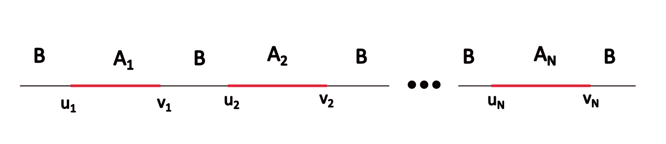
To set the stage for calculations later, we consider disjoint intervals whose boundary points are denoted and , see Figure 1. The length of each interval is denoted .
The organisation of this work is as follows. In Section 2 we discuss the symmetry-resolved Rényi entropy, and the multi-charged moments of theories with a global symmetry and also discuss the replica method for multi-charged moments in CFTs. In Section 3, we discuss the theory of free compact boson and review the Rényi entropy results in the theory. In Section 4, we evaluate the charged and multi-charged moments of free compact boson for multiple disjoint intervals. In Section 5, we evaluate the symmetry resolved Rényi entropy of free compact boson in the same settings. Finally, in Section 6 we give a conclusion of the present work. We also have four appendices. In Appendices A, B, and D some necessary computations and calculations are discussed. In Appendix C we evaluate the multi-charged moments of massless Dirac fermion for multiple disjoint intervals.
2 Symmetry resolution of Entanglement
In this section we discuss the symmetry resolution of Rényi entropy for theories with a global symmetry goldstein2018symmetry . We also discuss the charged and the multi-charged moments in the same context. Finally, we revisit the replica trick for evaluating the multi-charged moments in CFTs.
2.1 Symmetry Resolved Rényi Entropy
We consider a theory with a global internal symmetry and consider its bipartition into subsystem and its complement . Let the theory be in a state that satisfies , where is the density matrix and is the charge operator corresponding to the symmetry. Then for subsystem we have , where is the reduced density matrix and is the local charge operator in . This implies that is block diagonal in local charge sectors , here are the eigenvalues of . This allows us to study entanglement in local charge sectors , such studies have been termed symmetry-resolved entanglement.
The reduced density matrix in the charge sector , is defined as
| (2) |
where is the projection operator on to the charge sector and is the probability of the subsystem having the charge , mathematically . The Rényi entropies in these charge sectors are then defined as
| (3) |
The limit of (3) is the symmetry-resolved entanglement entropy. However, may not always be readily constructed, as is the case for our present interests. In such cases charge moments are introduced
| (4) |
Since, in the present case of our interest , it is also useful to define the more generalised quantities parez2021exact as
| (5) |
The operator in (5) is the local charge operator corresponding to the interval . The quantities have been termed multi-charged moments. Their utility will become clear in a moment. We denote by , the Fourier transforms of the multi-charged moments
| (6) |
The quantity is the joint probability of finding the charges in the subregions respectively. Similarly using (4), we also define the quantities as
| (7) |
The symmetry resolved Rényi entropy using is given by
| (8) |
We remark that the multi-charged moments given by (5) are also essential in the evaluation of symmetry-resolved mutual information, however, we do not consider symmetry-resolved mutual information in the present work.
2.2 Replica trick
We again consider the bipartite , and its complement and further assume that the theory is in its ground state. The moment of the reduced density matrix, is proportional to the partition function of the theory on the Replica surface ,
| (9) |
where is the partition function on the plane and is the euclidean Lagrangian of the theory. The surface is generally a Riemann surface. In our case, we are dealing with a theory with the decomposition . The corresponding Riemann surface has a genus .
When dealing with CFT’s it is particularly helpful to consider copies of the theory on the plane denoted and introduce the twist field calabrese2004entanglement ; cardy2008form . These twist fields correspond to the cyclic symmetry:
| (10) |
In this framework, the partition function is given by the correlation function of the twist fields,
| (11) |
The twist fields and are primary conformal fields with the scaling dimension calabrese2004entanglement
| (12) |
where is the central charge of the theory.
The presence of factors in eq.(5) modifies the boundary conditions between the different sheets on the Riemann surface . The multi-charged moments may be computed by introducing the flux-generating vertex operators goldstein2018symmetry . The operators generate the desired boundary conditions on the Riemann surface. The vertex operators and are placed on the boundary points and of the interval respectively, on the Riemann surface . The multi-charged moments are proportional to the correlation function
| (13) |
on the Riemann surface , where in the partition function on . Similarly the charged moments are given by
| (14) |
3 Free Compact Boson
In this section, we discuss the theory of free compact boson. We also revisit the results for the Rényi entropy of free compact boson when .
Free compact boson in is a conformally invariant theory with central charge . It is also the continuum theory of Luttinger liquid. The theory is described by the Lagrangian
| (15) |
The target space of the theory is a circle of circumference , where the compactification radius is related to the Luttinger parameter by . The theory has a duality under and is self-dual at . This duality is known as the T-duality.
Free compact boson possesses symmetry. The theory is invariant under the translations in the target space , this corresponds to a symmetry, sometimes denoted . The second symmetry is due to the conserved current in . We denote this second symmetry by . Under the T-duality we have the correspondence between the symmetries: and . In the present work we focus on at arbitrary compactification radius .
The Rényi entropy for two disjoint intervals case was first studied in furukawa2009mutual , and this result was generalised to arbitrary integer values of in calabrese2009entanglement2 . The Rényi entropies for multi-interval case was studied in coser2014renyi ; headrick2013bose . The moment of the reduced density matrix for arbitrary integer values of and is given by the generalised expression
| (16) |
where is a non-universal constant and are the cross-ratios
| (17) |
The factor comes from the local conformal algebra (i.e. it is not fixed by the global conformal invariance) and is a function of the cross-ratios (introduced later in eq.(25)). It is given by
| (18) |
In the above equation, is the Riemann Siegel theta function. A dimensional theta function is defined as
| (19) |
where the characteristics , and . In eq.(19) is a symmetric matrix with a positive definite imaginary part. When , the theta function in eq.(19) is denoted .
In eq.(18), is the Riemann period matrix associated with the Riemann surface of the moment of the reduced density matrix. It is a matrix, where is the genus of the Riemann surface. Let us write as
| (20) |
where and are real symmetric matrices. Then the matrix in eq.(18) is given by
| (21) |
where is the Luttinger parameter introduced earlier. We note from eq.(16), that is invariant under , as we would expect from the T-duality of compact boson. It has been noted in headrick2013bose , that at self-dual radius matches the corresponding of the Dirac fermion when in eq.(20) vanishes. This happens in particular for all values of when , and similarly for all values of when . It should also be noted that the factor becomes unity at self-dual radius when vanishes.
4 Multi-Charged moments
In this section, we obtain the multi-charged and charged moments of free compact boson for an arbitrary number of disjoint intervals.
The multi-charged moments of free compact boson in two disjoint intervals case for Rényi entropy was first obtained in ares2022multi , these moments were then used to study the symmetry resolved Rényi entropy and mutual information. In gaur2023charge , these quantities were obtained for Rényi negativity to study the symmetry-resolved Rényi negativity in the same settings.
The flux generating vertex operators in (13) for free compact boson are just the boson vertex operators goldstein2018symmetry
| (22) |
with the scaling dimension
| (23) |
To simplify our calculations we first use the global conformal invariance to map the points , , and using the map
| (24) |
Let’s denote the image of all the boundary points under this map as
| (25) |
where . We have the order and we also keep in mind the notations , , and . We must now compute the correlation function for the Vertex operators at on the Riemann surface (see Appendix A), i.e. . The Riemann surface has the genus . The correlation functions of vertex operators have been studied extensively in the string theory literature verlinde1987chiral ; eguchi1987chiral . A general point correlation function is given by
| (26) |
The map is a dimensional vector and is known as the Abel-Jacobi map. It is defined from the Riemann surface to its Jacobian torus . For the Riemann surface , we define its Jacobian lattice , where (given by eq.(79)) is the period matrix of . The Jacobian torus is then defined as the quotient space . The Abel-Jacobi map is given by
| (27) |
where , and and we have chosen as the reference point. The quantities are the normalised holomorphic differentials given by eq.(78) in Appendix A.
The quantity is the Prime form of the Riemann surface and is given by fay2006theta ; mumford2007tata
| (28) |
where , where , and were defined below eq.(19). However, here must be a non-singular odd half characteristic. The prime form is independent of the choice of . The quantity is a holomorphic 1-form and is given by
| (29) |
In our case, are the branch points and the normalised holomorphic differentials in eq.(29) are singular. This makes the vertex operator correlation function in eq.(26) ill-defined. This issue is resolved by introducing the regularised vertex operators ares2022multi . The normalised holomorphic differentials exhibit the leading order singular behaviour as
| (30) |
where is non-singular at the branch points. Using in eq.(29), and eq.(28) we may define the regularised holomorphic forms and regularised prime forms
| (31) | |||
| (32) |
This leads us to define the regularised Vertex operators
| (33) |
where is a surface-dependent constant. The constant will be fixed later, but we will find that it is independent of . The correlation function of the regularised vertex operators at branch points is well defined, and is given by
| (34) |
where . The flux is to be identified as , and in the equation above, where .
In the rest of this section, we will evaluate this correlation function for arbitrary values of and . We first revisit the two disjoint intervals case, we will use a different canonical homology basis than ares2022multi . We then extend these results to .
4.1 Two-interval case
The normalised holomorphic differential in the case of two disjoint intervals for arbitrary values of is evaluated by using eq.(76) in eq.(74), and eq.(78). It is given by
| (35) |
where is the hypergeometric function. The Abel-Jacobi map of the branch points is computed by using eq.(35) in eq.(27),
| (36) | ||||
| (37) | ||||
| (38) | ||||
| (39) |
where is given by
| (40) |
As noted earlier the normalised holomorphic differentials are singular at the branch points, and the corresponding non-singular is given by
| (41) |
where . Finally, the regularised prime forms are evaluated using eq.(41) in eq.(31) and eq.(32). These prime forms were conjectured to be simple algebraic functions in (ares2022multi, ),
| (42) | ||||
| (43) | ||||
| (44) |
where is a cross-ratio function on the Riemann surface and is given by
| (45) |
We numerically checked these conjectures for a few cases in Appendix B and found good agreement. The multi-charged moments are found by using eq.(36)-(39), and eq.(42)-(44) in eq.(34), and inverting the conformal transformation in eq.(24). In the limit of large separation between the two intervals, the multi-charged moments are just the product of the charged moments of two single intervals. This leads us to set the structure constant . The multi-charged moments are found to be
| (46) |
where is the non-universal constant and is given by eq.(16) without the non-universal constant. As expected, we find agreement with the known results of two-disjoint intervals.
4.2 Multi-interval case (N>2)
Let us first show that the exponential term in eq.(34) evaluates to unity. We show this by noting that if the condition
| (47) |
holds then the exponent in eq.(34) evaluates to zero. To argue this, consider when , and in eq.(34), the corresponding exponent vanishes if eq.(47) holds. Now, the exponent corresponding to , and , , is just the negative of when , and . Finally, we note that is given by
| (48) |
Then from eq.(47), we have , which completes our argument. Now to demonstrate that eq.(47) holds here, first we write from eq.(74), and eq.(78)
| (49) |
The matrix may be decomposed as follows coser2014renyi
| (50) |
where the matrix and the matrices are given by
| (51) | ||||
| (52) |
Note that our definition of and differs slightly from the reference. It then follows that also admits a similar decomposition, , were we have the relations and . The matrix is given by . Using these decompositions of , and in eq.(49) we obtain
| (53) |
This shows that the condition in eq.(45) is satisfied.
We now proceed to study the normalised holomorphic differentials at the branch points. As discussed earlier they are singular at the branch points. The quantities at the branch points are given by
| (54) | ||||
| (55) | ||||
| (56) |
where and in eq.(55). The matrices , and are the inverses of the matrices , and given by eq.(52). The regularised prime-forms are again given by using in eq.(31), and eq.(32). Following the two disjoint intervals case, we conjecture that the relatively complicated regularised prime forms are given by the simple algebraic functions
| (57) | ||||
| (58) | ||||
| (59) | ||||
| (60) |
where . The cross ratio functions are defined in eq.(45).
We checked these conjectures numerically for a few cases in Appendix B and found good agreement. There, however, arises a subtle issue of Riemann zeros in the numerical implementation of prime forms, this issue has been also discussed in Appendix B. The regularised vertex operator correlation function given by eq.(34) is evaluated to be
| (61) |
where , and on the left in the above equation are given below eq.(34). Finally, after taking the global conformal transformation, we obtain the multi-charged moments
| (62) |
where the cross-ratios are given by eq.(17) and we have introduced the non-universal constant . As before, is given by eq.(16) without the non-universal constant.
In ref.coser2014renyi it has been argued that in the limit of large separation between the intervals, the partition function factorises into the product of the partition function of the individual interval , i.e. =. We would expect this to hold for the multi-charged moments as well. This implies that we set . This also implies that the non-universal constant also factorises into the non-universal constant of each interval for arbitrary interval lengths and distances. The charged moments are similarly found to be
| (63) |
where we already used .
We may also study the limit of two intervals approaching each other in eq.(62) and eq.(63). To do so, let’s take the limit (i.e ), in this limit we have
| (64) |
where the must now be absorbed into the UV cut-off. This leads to a different non-universal constant in eq.(62) and eq.(63).
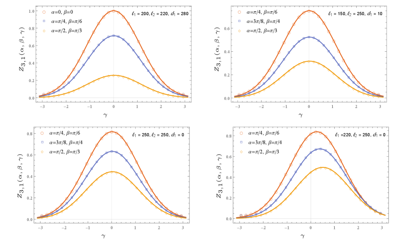
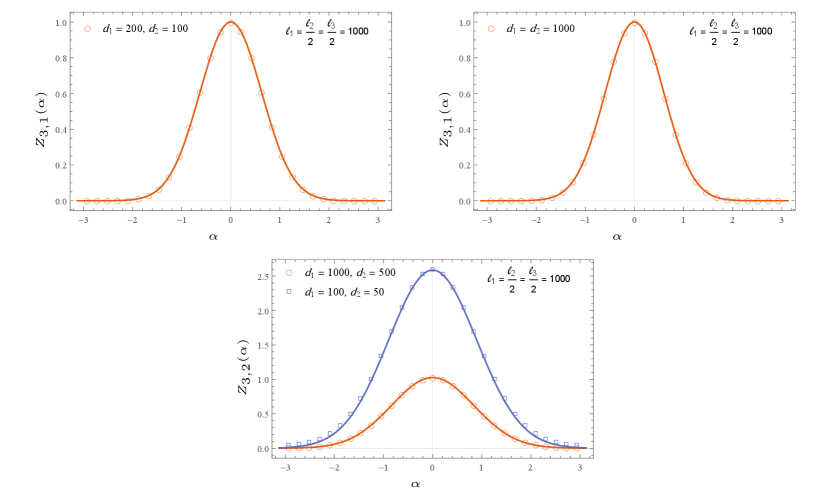
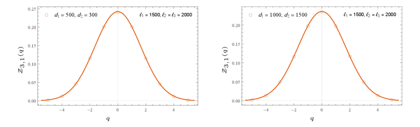
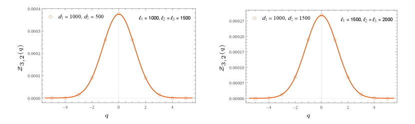
In Appendix C, we also computed the multi-charged moments for the d massless Dirac fermion in the same setting as well. We note that the multi-charged moments of compact boson at self-dual radius matches with that of massless Dirac fermions for the cases where the reduced density matrices of the two theory are known to match headrick2013bose . We also numerically checked our results for some of these cases against the tight-binding model, plots are shown in Figure 3 and Figure 4. The non-universal constant for the tight-binding model has been found in bonsignori2019symmetry . We see from the figures that we have a good numerical match.
5 Symmetry Resolved Rényi Entropy
In this section, we obtain the Symmetry resolved Rényi entropy and by taking the Fourier transform of the multi-charged and charged moments.
To evaluate the Fourier transform of the multi-charged moments we need the functional form of the non-universal constant in . In the last section, we argued that the non-universal constant for interval factorises into the product of the non-universal constant for the single interval. This allows us approximate the non-universal constant to the leading order in as xavier2018equipartition . We will use this approximation in the rest of this section.
To evaluate , let’s first introduce matrices for brevity later, defined as
| (65) |
We may write eq.(6) using eq.(63) and eq.(65), using our approximation of the non-universal
where we have introduced and . To evaluate this integral, we first take the Gaussian approximation of the integral. Then from the standard techniques for evaluating multi-variable Gaussian integral, we obtain
| (66) |
We note that the Luttinger parameter appears as an overall factor in the denominator of the exponent, promoting wider charge distribution. Similarly, we obtain in eq.(7) to be
| (67) |
where for brevity we introduced . The Luttinger parameter again appears as an overall factor in the denominator of the exponent and we see that the standard deviation is proportional to the Luttinger parameter. We have checked these results numerically against the tight-binding model in Figure 5 and Figure 6. Finally the symmetry resolved Rényi entropy is found to be
| (68) |
where is Rényi entropy of the free compact boson.
We see that to the leading order in , we have the familiar result of the equipartition of symmetry resolved Rényi entropy goldstein2018symmetry ; xavier2018equipartition . This equipartition is broken by the terms of , similar results have been obtained for free fermions on a lattice in bonsignori2019symmetry . Finally, the CFT result is given by
| (69) |
We also note that the Luttinger parameter appears in the terms. This generalises the symmetry-resolved Rényi entropy for the free compact boson for arbitrary disjoint intervals.
6 Conclusion
In this work, we evaluated the multi-charged moments and symmetry resolved Rényi entropy of free compact boson at arbitrary compactification radius for multiple disjoint intervals case. The symmetry resolved Rényi entropies were shown to have the familiar equipartition into the local charge sectors upto the leading order terms.
Free compact boson is the continuum theory of Luttinger liquids. The compactification radius of the free compact boson is related to the Luttinger parameter via . The charged and multi-charged moments of the theory are obtained by evaluating the correlation function of the flux-generating boson vertex operators placed at the branch points of the Riemann surface . The Riemann surface is the associated replica space and has a genus . The multi-charged moments are given in terms of relatively complicated prime forms of the Riemann surface . These expressions are however simplified to algebraic functions of interval lengths and distances using the conjectures made in eq.(57)-(60). Similar conjectures were first made in (ares2022multi, ) for the two disjoint intervals case. The symmetry resolved Rényi entropy was then obtained by evaluating the Fourier transform of the charged moments. In Appendix C the multi-charged moments of the massless Dirac field for multiple disjoint intervals were also evaluated. We found that the multi-charged moments of the self-dual compact boson and massless Dirac fermions match for the cases when the reduced density matrix of the two theories is known to match. Finally we also numerically checked out results for such cases against the tight-binding model. We found a good match between the analytical results and numerical evaluations.
Let’s now discuss some future outlooks for the present work. Rényi entropies studied in this work only account for the entanglement between the subsystem and its complement . To study the entanglement among the disjoint intervals mutual information measures are studied. These however are not measures of correlation, but still are interesting to study. The multi-charged moments obtained here are essential in the evaluation of symmetry-resolved mutual information parez2021exact . Symmetry-resolved entanglement has been studied for Dirac fermions on the torus foligno2023entanglement , and we believe that the results obtained here will prove to be useful in similar studies for free compact boson. Finally, the analytic results obtained here should be checked against the lattice models like d spin chains.
Appendix A Riemann Surfaces
In this section we review some topics in the theory of Riemann surfaces, particularly we focus on the normalised holomorphic differentials and the Riemann period matrix. For a detailed review, we refer the reader to fay2006theta ; mumford2007tata and to alvarez1987new ; alvarez1986riemann in the context of string theory.
We consider the singular Riemann surface , whose branch points are given by eq.(25). The Riemann surface has genus . This surface is parameterised by the curve
| (70) |
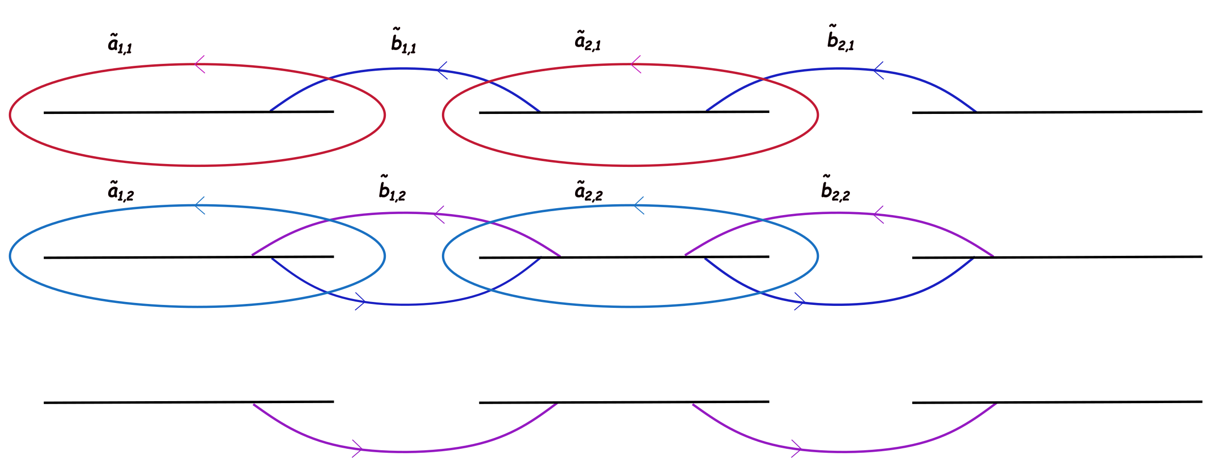
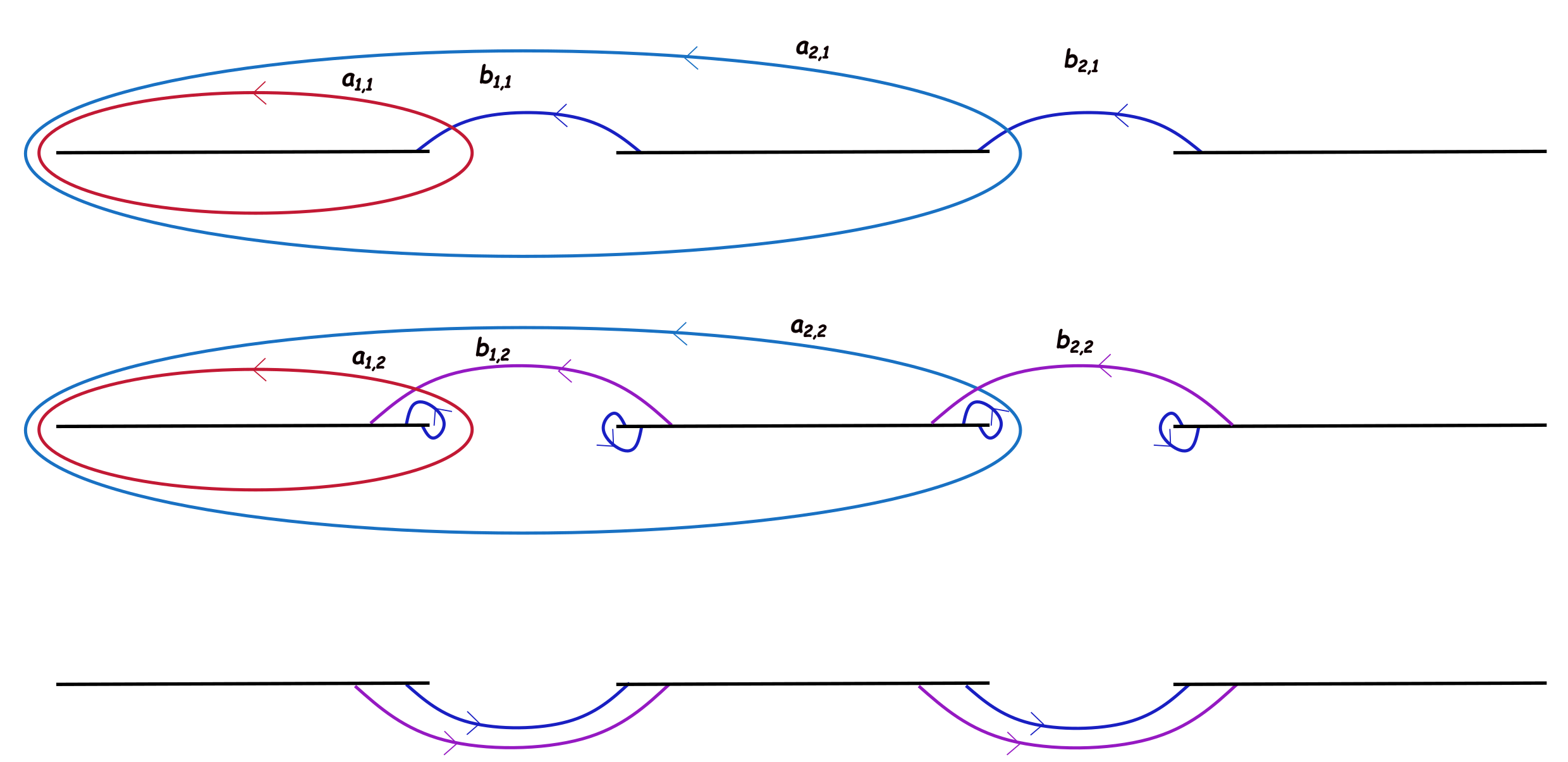
The period matrix can be given in a canonical homology basis on the Riemann surface. To proceed with our aim, we must choose a canonical homology basis on the Riemann surface. Following enolski2004singular , we first choose a set of auxiliary homology basis and, , where and . The non-contractible loop encloses the branch-cut on the sheet. The non-contractible loop goes through the branch-cut from the sheet to the sheet and returns to sheet through the branch-cut to close the loop. These loops do not form the canonical homology basis, since they do not satisfy the intersection conditions of the canonical homology basis
| (71) | ||||
| (72) |
Canonical homology basis may be constructed from the auxiliary basis using the following relations
| (73) |
Having chosen our canonical homology basis, we now proceed to introduce the matrices and . These matrices are defined as
| (74) | ||||
| (75) |
where are the basis of holomorphic differentials on . We define these holomorphic differentials as
| (76) |
The normalised holomorphic differentials are defined by the normalisation condition
| (77) |
We may construct the normalised holomorphic differentials using the holomorhic differentials , the normalised holomorphic differentials is given by
| (78) |
Finally, the period matrix associated with the Riemann surface is given by
| (79) |
The period matrix is the one which appears in the eq.(18), and eq.(20).
Appendix B Prime forms and cross-rations on Riemann surface
In this appendix, we numerically check the conjectures made in eq.(42)-(44), and eq.(57)-(60) for the regularised prime forms and cross-ratio function. We verified these conjectures numerically for a few cases and present the plots here.
N=2 case
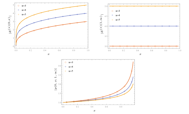
The conjectures for the case were first made in (ares2022multi, ), these conjectures were also proved for using the properties of Jacobi theta functions. Since we are using a different homology basis we numerically checked the conjectures for . We used the odd-half characteristics . These checks are plotted in Figure 9 and we see that we have a good match with the numerical results.
N>2 case
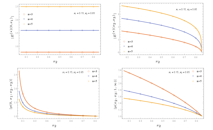
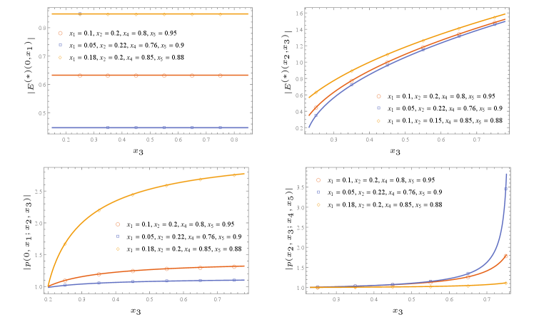
In these cases, we encounter Riemann zeros at some branch points of the Riemann surface for . Although the prime forms are independent of Riemann zeros, the numerical implementation of regularised prime forms becomes difficult. This problem is easily avoided by choosing the characteristics and wisely for each regularised prime form and cross-ratio function.
To give details, let’s first discuss the Riemann theorem. It states that given a Abel-Jacobi map defined from , the Riemann theta functions either vanishes for all or has zeros . Mathematically, we write
| (80) |
Furthermore, the zeros satisfy , where is a constant vector depending only upon the homology basis and the reference point . For odd-half characteristics, i.e , is always a Riemann zero. Let be a Riemann zero, however, if we now choose different odd-half characteristics and , then form eq.(19)
| (81) |
This means that is no longer necessarily a Riemann zero for new characteristics.
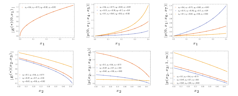
This allows us to deal with Riemann zeros at branch points during numerical implementation by choosing the characteristics wisely. While implementing the cross-ratio one must make sure that the characteristics on all the theta functions are the same. We have shown plots for a few cases for the numerical conjectures in eq.(57)-(60) in Figure 10, Figure 11, and Figure 12. We see from these figures that conjectures have a good match with the numerical results.
Appendix C Multi-charged moments for massless Dirac fermion
In this appendix, we evaluate the multi-charged moments of d massless Dirac fermions for multiple-disjoint intervals. The charged and multi-charged moments of d massless Dirac fermions have been studied in the single interval murciano2020entanglement and two disjoint intervals ares2022multi cases. The extension to multi-interval is relatively straightforward, but for the sake of completeness, we present these calculations in detail.
Massless Dirac fermion in d is a conformally invariant theory with central charge . Dirac fermions, however, unlike compact boson, are not modular invariant. The theory is described by the action
| (82) |
The gamma matrices are taken to be the Pauli matrices, and . Dirac fermions posses a symmetry under the transformation and .
To evaluate multi-charged moments for Dirac fermion we may consider n-copies of the field on the plane and introduce twist fields and casini2005entanglement ; murciano2020entanglement . The twist field act on the fields as
| (83) |
In this context is sometimes called the twist matrix. The multi-charge moments are given by the correlation function of twist fields placed on the boundary points of the intervals
| (84) |
We may decouple the -copies of the field by taking a unitary transformation that diagonalises the twist matrix. The eigenvalues of the twist matrix are , where . The field in this basis satisfies the following monodromy conditions around the boundary points
| (85) | ||||
| (86) |
The multi-charged moments in the new field basis are given by
| (87) |
where are the corresponding twist field which generates the monodromy condition in eq.(85), and eq.(86). The field may be written as casini2005entanglement . Here we have introduced single valued field and the gauge fields . It then follows from eq.(85), and eq.(86) that the gauge field satisfies
| (88) | ||||
| (89) |
Using the Stoke’s theorem, we deduce for eq.(88), and eq.(89) that
| (90) |
The multi-charged moments in eq.(87) are now just the product of the partition functions of the gauged fields . Multi-charged moments are now given by
| (91) |
We may evaluate the partition function using the bosonisation of the fermions, , where is the compact boson at compactfication radius . Using this duality the multi-charged moments may be written as the correlation function of the boson vertex operators ,
| (92) |
The correlation function of the vertex operators on the complex plane has been extensively studied in the literature, see for example francesco2012conformal . The neutrality condition, necessary for non-vanishing correlations, is satisfied by eq.(92). The multi-charged moments are then given by
| (93) |
where is just the reduced density matrix of disjoint interval for massless Dirac fermion. It is given by casini2005entanglement
| (94) |
Appendix D Numerical Model
In this appendix, we discuss the tight-binding model. Tight-binding model is the lattice theory of massless Dirac fermions. This model is used to perform the numerical checks against the analytical results in Section 4 and 5.
Tight-binding model is given by the Hamiltonian . The fermionic operators satisfies the commutation relations . This model has the correlation matrix , given by
| (95) |
The moments of the reduced density matrix is given by peschel2003calculation ; vidal2003entanglement
| (96) |
where are the eigenvalues of the correlation matrix restricted to subsystem (i.e. ).
Tight-binding model possesses a global symmetry. The corresponding conserved charge is given by . The charge moments, similar to eq.(96), are given by (parez2021exact, )
| (97) |
To find the multi-charge moment we first write the operator , where as a Gaussian operator, with the corresponding correlation matrix . The correlation matrix is given by
| (98) |
This leads to, using the algebra rules for Gaussian operators fagotti2010entanglement , the multi-charged moment
| (99) |
The matrix is given by
| (100) |
where the block matrices and the index . The matrix notation refers to the correlation matrix between the sites in with the sites in . The eq.(99)-(100) for have been used to plot the multi-charge moments in Figure 3, charged moments in Figure 4 and finally in Figure 5.
Acknowledgements.
HG is supported by the Prime Minister’s Research Fellowship offered by the Ministry of Education, Govt. of India. UY’s work is partly supported by Institute Chair Professorship of IIT Bombay.References
- [1] Michael A Nielsen and Isaac L Chuang. Quantum computation and quantum information. Cambridge university press, 2010.
- [2] Luigi Amico, Rosario Fazio, Andreas Osterloh, and Vlatko Vedral. Entanglement in many-body systems. Reviews of modern physics, 80(2):517, 2008.
- [3] Shinsei Ryu and Tadashi Takayanagi. Holographic derivation of entanglement entropy from the anti–de sitter space/conformal field theory correspondence. Physical review letters, 96(18):181602, 2006.
- [4] Shinsei Ryu and Tadashi Takayanagi. Aspects of holographic entanglement entropy. Journal of High Energy Physics, 2006(08):045, 2006.
- [5] Sergey N Solodukhin. Entanglement entropy of black holes. Living Reviews in Relativity, 14(1):1–96, 2011.
- [6] Guifre Vidal, José Ignacio Latorre, Enrique Rico, and Alexei Kitaev. Entanglement in quantum critical phenomena. Physical review letters, 90(22):227902, 2003.
- [7] Christoph Holzhey, Finn Larsen, and Frank Wilczek. Geometric and renormalized entropy in conformal field theory. Nuclear physics b, 424(3):443–467, 1994.
- [8] Pasquale Calabrese and John Cardy. Entanglement entropy and quantum field theory. Journal of statistical mechanics: theory and experiment, 2004(06):P06002, 2004.
- [9] Pasquale Calabrese and John Cardy. Entanglement entropy and conformal field theory. Journal of physics a: mathematical and theoretical, 42(50):504005, 2009.
- [10] Pasquale Calabrese, John Cardy, and Erik Tonni. Entanglement entropy of two disjoint intervals in conformal field theory. Journal of Statistical Mechanics: Theory and Experiment, 2009(11):P11001, 2009.
- [11] Andrea Coser, Luca Tagliacozzo, and Erik Tonni. On rényi entropies of disjoint intervals in conformal field theory. Journal of Statistical Mechanics: Theory and Experiment, 2014(1):P01008, 2014.
- [12] Shunsuke Furukawa, Vincent Pasquier, and Jun’ichi Shiraishi. Mutual information and boson radius in a c= 1 critical system in one dimension. Physical review letters, 102(17):170602, 2009.
- [13] Pasquale Calabrese, John Cardy, and Erik Tonni. Entanglement entropy of two disjoint intervals in conformal field theory: Ii. Journal of Statistical Mechanics: Theory and Experiment, 2011(01):P01021, 2011.
- [14] MA Rajabpour and Ferdinando Gliozzi. Entanglement entropy of two disjoint intervals from fusion algebra of twist fields. Journal of Statistical Mechanics: Theory and Experiment, 2012(02):P02016, 2012.
- [15] Vincenzo Alba, Luca Tagliacozzo, and Pasquale Calabrese. Entanglement entropy of two disjoint intervals in c= 1 theories. Journal of Statistical Mechanics: Theory and Experiment, 2011(06):P06012, 2011.
- [16] Andrea Coser, Erik Tonni, and Pasquale Calabrese. Spin structures and entanglement of two disjoint intervals in conformal field theories. Journal of Statistical Mechanics: Theory and Experiment, 2016(5):053109, 2016.
- [17] Maurizio Fagotti and Pasquale Calabrese. Entanglement entropy of two disjoint blocks in xy chains. Journal of Statistical Mechanics: Theory and Experiment, 2010(04):P04016, 2010.
- [18] Pasquale Calabrese, John Cardy, and Erik Tonni. Entanglement negativity in quantum field theory. Physical review letters, 109(13):130502, 2012.
- [19] Andrea Coser, Erik Tonni, and Pasquale Calabrese. Towards the entanglement negativity of two disjoint intervals for a one dimensional free fermion. Journal of Statistical Mechanics: Theory and Experiment, 2016(3):033116, 2016.
- [20] Matthew Headrick, Albion Lawrence, and Matthew Roberts. Bose–fermi duality and entanglement entropies. Journal of Statistical Mechanics: Theory and Experiment, 2013(02):P02022, 2013.
- [21] H Casini, CD Fosco, and M Huerta. Entanglement and alpha entropies for a massive dirac field in two dimensions. Journal of Statistical Mechanics: Theory and Experiment, 2005(07):P07007, 2005.
- [22] Moshe Goldstein and Eran Sela. Symmetry-resolved entanglement in many-body systems. Physical review letters, 120(20):200602, 2018.
- [23] JC Xavier, Francisco Castilho Alcaraz, and G Sierra. Equipartition of the entanglement entropy. Physical Review B, 98(4):041106, 2018.
- [24] Xhek Turkeshi, Paola Ruggiero, Vincenzo Alba, and Pasquale Calabrese. Entanglement equipartition in critical random spin chains. Physical Review B, 102(1):014455, 2020.
- [25] Riccarda Bonsignori, Paola Ruggiero, and Pasquale Calabrese. Symmetry resolved entanglement in free fermionic systems. Journal of Physics A: Mathematical and Theoretical, 52(47):475302, 2019.
- [26] Shachar Fraenkel and Moshe Goldstein. Symmetry resolved entanglement: exact results in 1d and beyond. Journal of Statistical Mechanics: Theory and Experiment, 2020(3):033106, 2020.
- [27] Filiberto Ares, Sara Murciano, and Pasquale Calabrese. Symmetry-resolved entanglement in a long-range free-fermion chain. Journal of Statistical Mechanics: Theory and Experiment, 2022(6):063104, 2022.
- [28] Nick G Jones. Symmetry-resolved entanglement entropy in critical free-fermion chains. Journal of Statistical Physics, 188(3):28, 2022.
- [29] Giuseppe Di Giulio and Johanna Erdmenger. Symmetry-resolved modular correlation functions in free fermionic theories. Journal of High Energy Physics, 2023(7), Jul 2023.
- [30] Hatem Barghathi, Emanuel Casiano-Diaz, and Adrian Del Maestro. Operationally accessible entanglement of one-dimensional spinless fermions. Physical Review A, 100(2):022324, 2019.
- [31] Hatem Barghathi, CM Herdman, and Adrian Del Maestro. Rényi generalization of the accessible entanglement entropy. Physical Review Letters, 121(15):150501, 2018.
- [32] Mostafa Ghasemi. Universal thermal corrections to symmetry-resolved entanglement entropy and full counting statistics. Journal of High Energy Physics, 2023(5):1–17, 2023.
- [33] Sara Murciano, Giuseppe Di Giulio, and Pasquale Calabrese. Entanglement and symmetry resolution in two dimensional free quantum field theories. Journal of High Energy Physics, 2020(8):1–42, 2020.
- [34] Sara Murciano, Giuseppe Di Giulio, and Pasquale Calabrese. Symmetry resolved entanglement in gapped integrable systems: a corner transfer matrix approach. SciPost Physics, 8(3):046, 2020.
- [35] Sara Murciano, Paola Ruggiero, and Pasquale Calabrese. Symmetry resolved entanglement in two-dimensional systems via dimensional reduction. Journal of Statistical Mechanics: Theory and Experiment, 2020(8):083102, 2020.
- [36] Filiberto Ares, Pasquale Calabrese, Giuseppe Di Giulio, and Sara Murciano. Multi-charged moments of two intervals in conformal field theory. Journal of High Energy Physics, 2022(9):1–37, 2022.
- [37] Alessandro Foligno, Sara Murciano, and Pasquale Calabrese. Entanglement resolution of free dirac fermions on a torus. Journal of High Energy Physics, 2023(3):1–45, 2023.
- [38] Luca Capizzi, Dávid X Horváth, Pasquale Calabrese, and Olalla A Castro-Alvaredo. Entanglement of the 3-state potts model via form factor bootstrap: total and symmetry resolved entropies. Journal of High Energy Physics, 2022(5):1–38, 2022.
- [39] Dávid X Horváth, Luca Capizzi, and Pasquale Calabrese. U (1) symmetry resolved entanglement in free 1+ 1 dimensional field theories via form factor bootstrap. Journal of High Energy Physics, 2021(5):1–40, 2021.
- [40] Luca Capizzi, Sara Murciano, and Pasquale Calabrese. Rényi entropy and negativity for massless complex boson at conformal interfaces and junctions. Journal of High Energy Physics, 2022(11):1–29, 2022.
- [41] Luca Capizzi, Sara Murciano, and Pasquale Calabrese. Rényi entropy and negativity for massless dirac fermions at conformal interfaces and junctions. Journal of High Energy Physics, 2022(8):1–35, 2022.
- [42] Luca Capizzi, Sara Murciano, and Pasquale Calabrese. Full counting statistics and symmetry resolved entanglement for free conformal theories with interface defects. arXiv preprint arXiv:2302.08209, 2023.
- [43] Gilles Parez, Riccarda Bonsignori, and Pasquale Calabrese. Exact quench dynamics of symmetry resolved entanglement in a free fermion chain. Journal of Statistical Mechanics: Theory and Experiment, 2021(9):093102, 2021.
- [44] Gilles Parez, Riccarda Bonsignori, and Pasquale Calabrese. Quasiparticle dynamics of symmetry-resolved entanglement after a quench: Examples of conformal field theories and free fermions. Physical Review B, 103(4):L041104, 2021.
- [45] Benoit Estienne, Yacine Ikhlef, and Alexi Morin-Duchesne. Finite-size corrections in critical symmetry-resolved entanglement. SciPost Physics, 10(3):054, 2021.
- [46] Luca Capizzi and Pasquale Calabrese. Symmetry resolved relative entropies and distances in conformal field theory. Journal of High Energy Physics, 2021(10):1–49, 2021.
- [47] Hui-Huang Chen. Symmetry decomposition of relative entropies in conformal field theory. Journal of High Energy Physics, 2021(7):1–25, 2021.
- [48] Aniket Rath, Vittorio Vitale, Sara Murciano, Matteo Votto, Jérôme Dubail, Richard Kueng, Cyril Branciard, Pasquale Calabrese, and Benoît Vermersch. Entanglement barrier and its symmetry resolution: Theory and experimental observation. PRX Quantum, 4(1):010318, 2023.
- [49] Sara Murciano, Jérôme Dubail, and Pasquale Calabrese. More on symmetry resolved operator entanglement. arXiv preprint arXiv:2309.04032, 2023.
- [50] Eyal Cornfeld, Moshe Goldstein, and Eran Sela. Imbalance entanglement: Symmetry decomposition of negativity. Physical Review A, 98(3):032302, 2018.
- [51] Sara Murciano, Riccarda Bonsignori, and Pasquale Calabrese. Symmetry decomposition of negativity of massless free fermions. SciPost Physics, 10(5):111, 2021.
- [52] Himanshu Gaur and Urjit A Yajnik. Charge imbalance resolved rényi negativity for free compact boson: Two disjoint interval case. Journal of High Energy Physics, 2023(2):1–26, 2023.
- [53] Hui-Huang Chen. Charged rényi negativity of massless free bosons. Journal of High Energy Physics, 2022(2):1–27, 2022.
- [54] Hui-Huang Chen. Dynamics of charge imbalance resolved negativity after a global quench in free scalar field theory. Journal of High Energy Physics, 2022(8):1–26, 2022.
- [55] Hui-Huang Chen and Zun-Xian Huang. Dynamics of charge imbalance resolved entanglement negativity after a local joining quench. arXiv preprint arXiv:2308.02868, 2023.
- [56] Noa Feldman and Moshe Goldstein. Dynamics of charge-resolved entanglement after a local quench. Physical Review B, 100(23):235146, 2019.
- [57] Gilles Parez, Riccarda Bonsignori, and Pasquale Calabrese. Dynamics of charge-imbalance-resolved entanglement negativity after a quench in a free-fermion model. Journal of Statistical Mechanics: Theory and Experiment, 2022(5):053103, 2022.
- [58] Clément Berthiere and Gilles Parez. Reflected entropy and computable cross-norm negativity: Free theories and symmetry resolution. Physical Review D, 108(5):054508, 2023.
- [59] Pasquale Calabrese, Jérôme Dubail, and Sara Murciano. Symmetry-resolved entanglement entropy in wess-zumino-witten models. Journal of High Energy Physics, 2021(10):1–32, 2021.
- [60] Giuseppe Di Giulio, René Meyer, Christian Northe, Henri Scheppach, and Suting Zhao. On the boundary conformal field theory approach to symmetry-resolved entanglement. SciPost Physics Core, 6(3):049, 2023.
- [61] Yuya Kusuki, Sara Murciano, Hirosi Ooguri, and Sridip Pal. Symmetry-resolved entanglement entropy, spectra & boundary conformal field theory. arXiv preprint arXiv:2309.03287, 2023.
- [62] Christian Northe. Entanglement resolution with respect to conformal symmetry. Phys. Rev. Lett., 131:151601, Oct 2023.
- [63] Suting Zhao, Christian Northe, and René Meyer. Symmetry-resolved entanglement in ads3/cft2 coupled to u (1) chern-simons theory. Journal of High Energy Physics, 2021(7):1–38, 2021.
- [64] Konstantin Weisenberger, Suting Zhao, Christian Northe, and René Meyer. Symmetry-resolved entanglement for excited states and two entangling intervals in ads3/cft2. Journal of High Energy Physics, 2021(12):1–31, 2021.
- [65] Suting Zhao, Christian Northe, Konstantin Weisenberger, and René Meyer. Charged moments in w3 higher spin holography. Journal of High Energy Physics, 2022(5):1–28, 2022.
- [66] Alexandre Belin, Ling-Yan Hung, Alexander Maloney, Shunji Matsuura, Robert C Myers, and Todd Sierens. Holographic charged rényi entropies. Journal of High Energy Physics, 2013(12):1–50, 2013.
- [67] Alexey Milekhin and Amirhossein Tajdini. Charge fluctuation entropy of hawking radiation: a replica-free way to find large entropy. arXiv preprint arXiv:2109.03841, 2021.
- [68] Himanshu Gaur and Urjit A Yajnik. Symmetry resolved entanglement entropy in hyperbolic de sitter space. Physical Review D, 107(12):125008, 2023.
- [69] Antoine Neven, Jose Carrasco, Vittorio Vitale, Christian Kokail, Andreas Elben, Marcello Dalmonte, Pasquale Calabrese, Peter Zoller, Benoit Vermersch, Richard Kueng, et al. Symmetry-resolved entanglement detection using partial transpose moments. npj Quantum Information, 7(1):152, 2021.
- [70] Márton Kormos and Zoltán Zimborás. Temperature driven quenches in the ising model: appearance of negative rényi mutual information. Journal of Physics A: Mathematical and Theoretical, 50(26):264005, 2017.
- [71] John L Cardy, Olalla A Castro-Alvaredo, and Benjamin Doyon. Form factors of branch-point twist fields in quantum integrable models and entanglement entropy. Journal of Statistical Physics, 130:129–168, 2008.
- [72] Erik Verlinde and Herman Verlinde. Chiral bosonization, determinants and the string partition function. Nuclear Physics B, 288:357–396, 1987.
- [73] Tohru Eguchi and Hirosi Ooguri. Chiral bosonization on a riemann surface. Physics Letters B, 187(1-2):127–134, 1987.
- [74] John D Fay. Theta functions on Riemann surfaces, volume 352. Springer, 2006.
- [75] David Mumford, Madhav Nori, and Peter Norman. Tata lectures on theta III, volume 43. Springer, 2007.
- [76] Luís Alvarez-Gaumé, C Gomez, and C Reina. New methods in string theory. Technical report, 1987.
- [77] Luís Alvarez-Gaumé and P Nelson. Riemann surfaces and string theories. Technical report, 1986.
- [78] Victor Z Enolski and Tamara Grava. Singular zn-curves and the riemann-hilbert problem. International Mathematics Research Notices, 2004(32):1619–1683, 2004.
- [79] Philippe Francesco, Pierre Mathieu, and David Sénéchal. Conformal field theory. Springer Science & Business Media, 2012.
- [80] Ingo Peschel. Calculation of reduced density matrices from correlation functions. Journal of Physics A: Mathematical and General, 36(14):L205, 2003.