This paper was converted on www.awesomepapers.org from LaTeX by an anonymous user.
Want to know more? Visit the Converter page.

Multi-agent system for target tracking on a sphere and its asymptotic behavior

Sun-Ho Choi Department of Applied Mathematics and the Institute of Natural Sciences, Kyung Hee University, 1732 Deogyeong-daero, Giheung-gu, Yongin 17104, Republic of Korea [email protected] Dohyun Kwon Department of Mathematics, University of Wisconsin-Madison, 480 Lincoln Dr., Madison, WI 53706, USA [email protected]  and  Hyowon Seo Department of Applied Mathematics and the Institute of Natural Sciences, Kyung Hee University, 1732 Deogyeong-daero, Giheung-gu, Yongin 17104, Republic of Korea [email protected]
Abstract.

We propose a second-order multi-agent system for target tracking on a sphere. The model contains a centripetal force, a bonding force, a velocity alignment operator to the target, and cooperative control between flocking agents. We propose an appropriate regularized rotation operator instead of Rodrigues’ rotation operator to derive the velocity alignment operator for target tracking. By the regularized rotation operator, we can decompose the phase of agents into translational and structural parts. By analyzing the translational part of this reference frame decomposition, we can obtain rendezvous results to the given target. If the multi-agent system can obtain the target’s position, velocity, and acceleration vectors, then the complete rendezvous occurs. Even in the absence of the target’s acceleration information, if the coefficients are sufficiently large enough, then the practical rendezvous occurs.

1. Introduction

Target tracking refers to designing a dynamical system that agents follow given maneuvering target agents using the information of the targets, such as position, velocity, and acceleration. The target tracking problem is applied in various fields, such as mobile sensor networks, virtual reality, and surveillance systems using unmanned aerial vehicles (UAVs) [18, 22, 24]. Most of the relevant literature focuses on the uncertainty of target motions. From a technical point of view, we can divide the models for this field into measurement models, target motion models, and filtering models. The measurement model deals with target information in a sensor coordinate containing additive noise such as image sensors and radar sensor networks [2, 3, 20]. The target motion model is a coupled dynamical system for target tracking. The filtering model is based on the particle filter method and stochastic frameworks estimating the target state such as nonlinear filtering [13, 15] and adaptive filtering [14, 16].

Depending on the structure of the system, we also divide the models for target tracking into two types of systems: single integrator model and double integrator model. For the single integrator model, one can control the velocity of the agents directly. For example, in [10], the authors proposed a tracking algorithm for a slowly moving target using the target’s position and bearing angle. Many researchers assume agents can obtain only the target’s position and bearing angle for targets maneuvering underwater. From the engineering point of view, it is a reasonable assumption. For the double integrator model, one can control the acceleration of agents. After Olfati-Saber’s seminal work [11], researches for the dynamic tracking system using the double integrator model have been extensively conducted. For this kind of model, the tracking agents can have the position and velocity information of the target. Moreover, to avoid collisions between agents or make a formation flight of the agents, a flocking algorithm and cooperative control are frequently used.

The domain or manifolds of agents are also one of the main topics in this field [1, 18] such as the surveillance system for the restricted area or target tracking system on the whole planet. Our goal is to provide a robust navigational feedback system for the target tracking problem on a sphere. Let γ\gamma-agent be a given target governed by the following system:

q˙γ=pγ,p˙γ=pγ2qγ2qγ+Uγ(t),\displaystyle\begin{aligned} \dot{q}_{\gamma}&=p_{\gamma},\\ \dot{p}_{\gamma}&=-\frac{\|p_{\gamma}\|^{2}}{\|q_{\gamma}\|^{2}}q_{\gamma}+U_{\gamma}(t),\end{aligned} (1.1)

where qγ𝕊2q_{\gamma}\in\mathbb{S}^{2}, pγTqγ𝕊2p_{\gamma}\in T_{q_{\gamma}}\mathbb{S}^{2}, and UγU_{\gamma} are the position, velocity, and control law of the target agent (γ\gamma-agent) on sphere, respectively. To conserve the modulus of qγ(t)𝕊2q_{\gamma}(t)\in\mathbb{S}^{2}, we additionally assume that the following condition holds for all t0t\geq 0.

qγ(t)Uγ(t).q_{\gamma}(t)\perp U_{\gamma}(t).

Therefore, the control law Uγ(t)U_{\gamma}(t) has the following form: for some uγ(t)3u_{\gamma}(t)\in\mathbb{R}^{3},

Uγ(t)=qγ(t)2uγ(t)uγ(t),qγ(t)qγ(t).U_{\gamma}(t)=\|q_{\gamma}(t)\|^{2}u_{\gamma}(t)-\langle u_{\gamma}(t),q_{\gamma}(t)\rangle q_{\gamma}(t).

For simplicity, we assume that uγ(t)u_{\gamma}(t) is continuous.

For a given γ\gamma-agent, we propose a novel multi-agent system for the target tracking on a spherical space:

q˙i(t)=pi(t),p˙i(t)=pi2qi2qi+j=1NσijN(qi2qjqi,qjqi)+cq(qi2qγqi,qγqi)+cp(Pqγqi(pγ)pi)+Ui,\displaystyle\begin{aligned} \dot{q}_{i}(t)&=p_{i}(t),\\ \dot{p}_{i}(t)&=-\frac{\|p_{i}\|^{2}}{\|q_{i}\|^{2}}q_{i}+\sum_{j=1}^{N}\frac{\sigma_{ij}}{N}(\|q_{i}\|^{2}q_{j}-\langle q_{i},q_{j}\rangle q_{i})\\ &\quad+c_{q}(\|q_{i}\|^{2}q_{\gamma}-\langle q_{i},q_{\gamma}\rangle q_{i})+c_{p}({P}_{q_{\gamma}\rightarrow q_{i}}(p_{\gamma})-p_{i})+U_{i},\end{aligned} (1.2)

where qi𝕊2q_{i}\in\mathbb{S}^{2} and piTqi𝕊2p_{i}\in T_{q_{i}}\mathbb{S}^{2} are the position and velocity of the iith agent, respectively. The first term on the right-hand side of the second equation is the centripetal force term to conserve the modulus of qiq_{i}. The second term

j=1NσijN(qi2qjqi,qjqi)\sum_{j=1}^{N}\frac{\sigma_{ij}}{N}(\|q_{i}\|^{2}q_{j}-\langle q_{i},q_{j}\rangle q_{i})

is the cooperative control term between agents where the inter-particle force parameter is given by

σij=σ(xixj2).\displaystyle\sigma_{ij}=\sigma(\|x_{i}-x_{j}\|^{2}).

The next two terms, cq(qi2qγqi,qγqi)c_{q}(\|q_{i}\|^{2}q_{\gamma}-\langle q_{i},q_{\gamma}\rangle q_{i}) and cp(Pqγqi(pγ)pi)c_{p}({P}_{q_{\gamma}\rightarrow q_{i}}(p_{\gamma})-p_{i}), are the bonding force and a velocity alignment term between the target and the iith agent, respectively, where cq>0c_{q}>0 and cp>0c_{p}>0 are target tracking coefficients for the position and velocity, respectively. The last term UiU_{i} is an extra control law based on the target’s information, which will be determined later in (1.5) and (1.6) for each purpose.

Throughout this paper, we assume the initial data satisfies the following admissible conditions on 𝕊2\mathbb{S}^{2}:

qi(0)=1,pi(0),qi(0)=0, for all i{1,,N}.\displaystyle\|q_{i}(0)\|=1,\quad\langle p_{i}(0),q_{i}(0)\rangle=0,\quad\mbox{ for all $i\in\{1,\ldots,N\}$}. (1.3)
Definition 1.1.

For a given target (qγ(t),pγ(t))(q_{\gamma}(t),p_{\gamma}(t)), let {(qi(t),pi(t))}i=1N\{(q_{i}(t),p_{i}(t))\}_{i=1}^{N} be the solution to (1.2). We define the two kinds of rendezvouses.

  1. (1)

    An asymptotic complete rendezvous occurs between the agents and the given target, if

    limtmax1iNqi(t)qγ(t)=0.\lim_{t\to\infty}\max_{1\leq i\leq N}\|q_{i}(t)-q_{\gamma}(t)\|=0.
  2. (2)

    An asymptotic practical rendezvous occurs between the agents and the given target, if

    limcq,cplimtmax1iNqi(t)qγ(t)=0.\lim_{c_{q},c_{p}\to\infty}\lim_{t\to\infty}\max_{1\leq i\leq N}\|q_{i}(t)-q_{\gamma}(t)\|=0.

In what follows, we will show that our model contains many robust properties, including the complete rendezvous. Even in the absence of the target acceleration information, the practical rendezvous occurs when the coefficients are large enough. In particular, we obtain a sharp estimate of the distance between the target and agents. There are many other papers on the dynamics on 𝕊2\mathbb{S}^{2} as well as n\mathbb{R}^{n}, but our asymptotic analysis including exponential convergence and practical rendezvous is new on the target tracking problem, to the best of our knowledge.

The derivation of our model is motivated by the decomposition property of flocking dynamics on a flat space. On a flat space, from momentum conservation, the dynamics is represented by the composition of frame reference dynamics and local alignment dynamics as in [11]. In contrast to previous results in n\mathbb{R}^{n}, it is hard to expect such a decomposition for the flocking model on 𝕊2\mathbb{S}^{2}. See Sections 2 and 3 for details. In particular, in our previous papers [6, 7, 8], we used Rodrigues’ rotation operator R{R_{\cdot\rightarrow\cdot}} to derive a flocking system on a sphere since Rodrigues’ rotation operator R{R_{\cdot\rightarrow\cdot}} is the most natural flocking operator. However, its composition is complex so that it is difficult to analyze. Moreover, it contains an unavoidable singularity at antipodal points due to its geometric characteristics. From this singularity, even though agents are located on 𝕊2\mathbb{S}^{2}, the vanishing point on the communication rate is necessary [6]. Due to this difficulty, the target tracking problem on 𝕊2\mathbb{S}^{2} has not been well understood.

We remove the singular term from the natural rotation operator R{R_{\cdot\rightarrow\cdot}} to obtain a rotation operator in two dimensions:

Pz1z2:=z1,z2I+z2z1Tz1z2T, for z1 and z2 in a unit sphere.\displaystyle{P}_{z_{1}\rightarrow z_{2}}:=\langle z_{1},z_{2}\rangle I+z_{2}z_{1}^{T}-z_{1}z_{2}^{T},\quad\hbox{ for $z_{1}$ and $z_{2}$ in a unit sphere. } (1.4)

See also Appendix A for the motivation of the non-singularity rotation operator PP and its properties. We will prove that its dynamics consists of the composition of the rigid motion part on 𝕊2\mathbb{S}^{2} and the local alignment part. Using this property, we derive an 𝕊2\mathbb{S}^{2}-version of the reference frame decomposition in Proposition 3.2 and provide a sufficient condition to obtain a target tracking estimate between multiple agents {(qi(t),pi(t))}i=1N\{(q_{i}(t),p_{i}(t))\}_{i=1}^{N} and the given target (qγ(t),pγ(t))(q_{\gamma}(t),p_{\gamma}(t)). Moreover, by the regularity of the operator P{P}, we can obtain the following global existence result.

Theorem 1.

Assume that for a continuous function uγu_{\gamma}, a given target (qγ(t),pγ(t))(q_{\gamma}(t),p_{\gamma}(t)) satisfies (1.1). If the initial data {(qi(0),pi(0))}i=1N\{(q_{i}(0),p_{i}(0))\}_{i=1}^{N} satisfies (1.3) and UiU_{i} is Lipschitz continuous with respect to {(qi,pi)}i=1N\{(q_{i},p_{i})\}_{i=1}^{N} with Ui,qi=0\langle U_{i},q_{i}\rangle=0, then there exists a unique global-in-time solution {(qi(t),pi(t))}i=1N\{(q_{i}(t),p_{i}(t))\}_{i=1}^{N} to system (1.2) and {qi(t)}i=1N\{q_{i}(t)\}_{i=1}^{N} are located on 𝕊2\mathbb{S}^{2} for all time t>0t>0.

As in d\mathbb{R}^{d}, we notice that the velocity alignment operator between the target and the agents plays an important role in target tracking. In particular, the bonding force between the target and the agents, cq(qi2qγqi,qγqi)c_{q}(\|q_{i}\|^{2}q_{\gamma}-\langle q_{i},q_{\gamma}\rangle q_{i}), alone is not enough to track a target on 𝕊2\mathbb{S}^{2}. The velocity alignment operator cp(Pqγqi(pγ)pi)c_{p}({P}_{q_{\gamma}\rightarrow q_{i}}(p_{\gamma})-p_{i}) is crucial for the target tracking algorithm. See the simulations in Section 5. In the next two theorems, we present a quantitative analysis of the velocity alignment operator with two different UiU_{i}’s;

Ui=2wγ,qi(qi×pi)+w˙γ(t)×qi\displaystyle U_{i}=2\langle w_{\gamma},q_{i}\rangle(q_{i}\times p_{i})+\dot{w}_{\gamma}(t)\times q_{i} (1.5)

or

Ui=0,\displaystyle U_{i}=0, (1.6)

where wγw_{\gamma} is the angular velocity of the target given by

wγ=qγ×pγ.\displaystyle w_{\gamma}=q_{\gamma}\times p_{\gamma}. (1.7)

From Theorem 2, if the agents can obtain the exact target information containing acceleration, then the agents can accurately track the target, and the position differences between the target and the agents decay exponentially fast.

Theorem 2.

Let (qγ(t),pγ(t))(q_{\gamma}(t),p_{\gamma}(t)) be a given target satisfying (1.1) with a continuous target control uγu_{\gamma} and {qi(t),pi(t)}i=1N\{q_{i}(t),p_{i}(t)\}_{i=1}^{N} be the solution to (1.2) satisfying (1.3). We assume that σij=σ\sigma_{ij}=\sigma is a positive constant and

Ui=2wγ,qi(qi×pi)+w˙γ(t)×qi,U_{i}=2\langle w_{\gamma},q_{i}\rangle(q_{i}\times p_{i})+\dot{w}_{\gamma}(t)\times q_{i},

where wγw_{\gamma} is the angular velocity defined in (1.7).

If cq>σ>0c_{q}>\sigma>0 or

1Ni=1Npi(0)wγ(0)×qi(0)2\displaystyle\frac{1}{N}\sum_{i=1}^{N}\|p_{i}(0)-w_{\gamma}(0)\times q_{i}(0)\|^{2}
+σ2N2i,j=1Nqi(0)qj(0)2+cqNi=1Nqγ(0)qi(0)2<σ(1+cqσ)2,\displaystyle\quad+\frac{\sigma}{2N^{2}}\sum_{i,j=1}^{N}\|q_{i}(0)-q_{j}(0)\|^{2}+\frac{c_{q}}{N}\sum_{i=1}^{N}\|q_{\gamma}(0)-q_{i}(0)\|^{2}<\sigma\left(1+\frac{c_{q}}{\sigma}\right)^{2},

then the asymptotic complete rendezvous occurs and its convergence rate is exponential, i.e., there are positive constants 𝒞\mathcal{C}, 𝒟\mathcal{D} such that

qi(t)qγ(t),pi(t)pγ(t)𝒞e𝒟t.\|q_{i}(t)-q_{\gamma}(t)\|,~{}\|p_{i}(t)-p_{\gamma}(t)\|\leq\mathcal{C}e^{-\mathcal{D}t}.
Remark 1.1.
  1. (1)

    If the above sufficient condition in Theorem 2 does not hold, then we can find a steady-state solution. This means that the sufficient condition is almost optimal to lead the convergence result in Theorem 2. See Section 5.

  2. (2)

    The author in [11] does not deal with the estimate of the distance between the target and agents. Our model is inspired by [11], but the target tracking estimate and practical rendezvous are novel.

  3. (3)

    The derivation of UiU_{i} in the above theorem is technical, but from the frame decomposition in Proposition 3.2, it is a very natural choice to obtain the complete rendezvous.

The former one in (1.5) corresponds to the case with the target acceleration, while it is unknown in the latter case (1.6). These choices with the different amounts of the target information induce the different accuracies of the target tracking. Since the target information obtained by the agents through observation is usually incomplete, there have been many studies to overcome this incompleteness. For example, many researchers proposed target tracking systems including restricted target information [10, 19], communication-induced delays [12, 17], and additive noise from measurement [9, 23]. The result in Theorem 3 below means that the large coefficients of the system allow the agents to get close enough to the target as needed without acceleration information of the target. In other words, the practical rendezvous occurs.

Theorem 3.

For (qγ(t),pγ(t))(q_{\gamma}(t),p_{\gamma}(t)) satisfying (1.1) with a continuous target control uγu_{\gamma}, let {qi(t),pi(t)}i=1N\{q_{i}(t),p_{i}(t)\}_{i=1}^{N} be the solution to (1.2) subject to the initial data satisfying (1.3) and

Ui=0.U_{i}=0.

Assume that σij=σ\sigma_{ij}=\sigma is a positive constant and the angular velocity of the target and its time derivative are bounded

wγ,w˙γ<Cγ.\|w_{\gamma}\|,\|\dot{w}_{\gamma}\|<C_{\gamma}.

If pi(0)pγ(0)2\|p_{i}(0)-p_{\gamma}(0)\|\neq 2 for all i{1,,N}i\in\{1,\ldots,N\}, then the asymptotic practical rendezvous occurs and

qi(t)qγ(t)𝒞e𝒟4t+𝒞𝒟,\|q_{i}(t)-q_{\gamma}(t)\|\leq\mathcal{C}e^{-\frac{\mathcal{D}}{4}t}+\frac{\mathcal{C}}{\mathcal{D}},

where 𝒞\mathcal{C} is a positive constant depending on the initial data, σ\sigma, and CγC_{\gamma}. The constant 𝒟\mathcal{D} is given by

𝒟:={cp4cq+cp2,ifcp24cq,cp,ifcp2<4cq.\displaystyle\mathcal{D}:=\left\{\begin{array}[]{ll}\displaystyle~{}c_{p}-\sqrt{-4c_{q}+c_{p}^{2}},&\quad\mbox{if}\quad c_{p}^{2}\geq-4c_{q},\\ \displaystyle~{}c_{p},&\quad\mbox{if}\quad c_{p}^{2}<-4c_{q}.\end{array}\right.

There are technical issues in the proofs of Theorems 2 and 3. We can obtain the complete rendezvous result in Theorem 2 through Lasalle’s invariance principle with an energy functional. However, Lasalle’s invariance principle does not give a convergence rate. An appropriate Lyapunov functional will be used to obtain the exponential convergence result. In particular, in this case, we derive a closed differential inequality by using six functionals including information on the distance between the target and agents and the distance between agents. The practical rendezvous in Theorem 3 has a more subtle issue. It is necessary to control the distance between the target and agents through the size of the coefficients. However, it is impossible if the coefficients appear in the nonlinear higher-order terms except for the linear terms. If we use a standard functional, the coefficients necessarily occur in the nonlinear terms due to the geometrical characteristics of 𝕊2\mathbb{S}^{2}. This problem will be solved by using new functionals inspired by hyperbolic geometry.

The rest of the paper is organized as follows. In Section 2, we present the global-in-time existence and uniqueness of the solution to (1.2) and target tracking results for 3\mathbb{R}^{3}. Section 3 is devoted to a reference frame decomposition for the main system. From this decomposition, the solution to the main system is represented by the composition of operators for the translational part and the structural part. Next, we reduce the system for the structural part to a linearized system in Section 4. Using this, we prove the complete and practical rendezvouses of Theorems 2 and 3 in Section 5. In Section 6, we verify our analytic results using numerical simulations. Section 7 is devoted to the summary of our results.

2. Preliminary: Global well-posedness and Motivations

2.1. The global existence and uniqueness

In this section, we provide the proof of Theorem 1: there is a unique global-in-time solution to (1.2) and this solution is located on the sphere when the initial data satisfies the admissible conditions in (1.3).

For the local existence and uniqueness, we use the same argument in [6, 7]. For given C1C^{1} functions qγq_{\gamma}, pγp_{\gamma}, and wγ=qγ×pγw_{\gamma}=q_{\gamma}\times p_{\gamma}, we consider the following system of ODEs:

q˙i(t)=pi(t),p˙i(t)=pi2qi2qi+j=1Nσ(xixj2)N(qi2qjqi,qjqi)+cq(qi2qγqi,qγqi)+cp(qγ,qipγqi,pγqγpi)+Ui.\displaystyle\begin{aligned} \dot{q}_{i}(t)&=p_{i}(t),\\ \dot{p}_{i}(t)&=-\frac{\|p_{i}\|^{2}}{\|q_{i}\|^{2}}q_{i}+\sum_{j=1}^{N}\frac{\sigma(\|x_{i}-x_{j}\|^{2})}{N}(\|q_{i}\|^{2}q_{j}-\langle q_{i},q_{j}\rangle q_{i})\\ &\quad+c_{q}(\|q_{i}\|^{2}q_{\gamma}-\langle q_{i},q_{\gamma}\rangle q_{i})+c_{p}(\langle q_{\gamma},q_{i}\rangle p_{\gamma}-\langle q_{i},p_{\gamma}\rangle q_{\gamma}-p_{i})+U_{i}.\end{aligned} (2.1)

Here, we will choose Ui=2wγ,qi(qi×pi)+w˙γ(t)×qiU_{i}=2\langle w_{\gamma},q_{i}\rangle(q_{i}\times p_{i})+\dot{w}_{\gamma}(t)\times q_{i} for the complete rendezvous and Ui=0U_{i}=0 for the practical rendezvous.

We assume that the initial data {(qi(0),pi(0))}i=1N\{(q_{i}(0),p_{i}(0))\}_{i=1}^{N} satisfies the admissible condition in (1.3). Then the right-hand side of (2.1) is Lipschitz continuous with respect to {(qi,pi)}i=1N\{(q_{i},p_{i})\}_{i=1}^{N} in a small neighborhood of {(qi(0),pi(0))}i=1N\{(q_{i}(0),p_{i}(0))\}_{i=1}^{N} in 6N\mathbb{R}^{6N}. By the Picard-Lindelöf Theorem, there is the maximum time interval [0,TM)[0,T_{M}) in which a solution of (2.1) exists and it is unique.

We next follow the same argument in [6, 7]. On the maximum time interval [0,TM)[0,T_{M}), we take the inner product between the second equation of (2.1) and xix_{i} to obtain that

p˙i,qi\displaystyle\langle\dot{p}_{i},q_{i}\rangle =pi2cppi,qi.\displaystyle=-\|p_{i}\|^{2}-c_{p}\langle p_{i},q_{i}\rangle. (2.2)

By (2.2) and the first equation of (2.1), we obtain that

ddti=1N|pi,qi|2\displaystyle\frac{d}{dt}\sum_{i=1}^{N}|\langle p_{i},q_{i}\rangle|^{2} =2i=1N(p˙i,qi+pi,q˙i)pi,qi\displaystyle=2\sum_{i=1}^{N}(\langle\dot{p}_{i},q_{i}\rangle+\langle p_{i},\dot{q}_{i}\rangle)\langle p_{i},q_{i}\rangle
=2i=1N(p˙i,qi+pi2)pi,qi\displaystyle=2\sum_{i=1}^{N}(\langle\dot{p}_{i},q_{i}\rangle+\|p_{i}\|^{2})~{}\langle p_{i},q_{i}\rangle
=2cpi=1N|pi,qi|2.\displaystyle=-2c_{p}\sum_{i=1}^{N}|\langle p_{i},q_{i}\rangle|^{2}.

Note that the initial data satisfies i=1N|vi(0),xi(0)|2=0\sum_{i=1}^{N}|\langle v_{i}(0),x_{i}(0)\rangle|^{2}=0. Therefore, the Gronwall inequality implies that

i=1N|vi(t),xi(t)|0,fort>0,\displaystyle\sum_{i=1}^{N}|\langle v_{i}(t),x_{i}(t)\rangle|\equiv 0,\quad\mbox{for}~{}t>0,

and this implies that

vi(t),xi(t)0.\displaystyle\langle v_{i}(t),x_{i}(t)\rangle\equiv 0.

We take the inner product between q˙i\dot{q}_{i} and qiq_{i}. By the first equation of (2.1),

ddtqi2=2q˙i,qi=2pi,qi=0.\displaystyle\frac{d}{dt}\|q_{i}\|^{2}=2\langle\dot{q}_{i},q_{i}\rangle=2\langle p_{i},q_{i}\rangle=0.

Since initial conditions satisfy xi(0)=1\|x_{i}(0)\|=1 and vi(0),xi(0)=0\langle v_{i}(0),x_{i}(0)\rangle=0 for all i{1,,N}i\in\{1,\ldots,N\}, we have

xi(t)1,fort>0,i{1,N}.\displaystyle\|x_{i}(t)\|\equiv 1,\quad\mbox{for}~{}t>0,~{}i\in\{1,\ldots N\}.

In conclusion, we can apply the extensibility of solutions in [21, Corollary 2.2] to obtain that

TM=.T_{M}=\infty.

Moreover, we can easily check that {(qi(t),pi(t))}i=1N\{(q_{i}(t),p_{i}(t))\}_{i=1}^{N} is the unique solution to (1.2) by a standard argument. Therefore, we can obtain the following proposition.

Proposition 2.1.

Let {(qi(t),pi(t))}i=1N\{(q_{i}(t),p_{i}(t))\}_{i=1}^{N} be a solution to (1.2) with (1.3). Then for all i{1,,N}i\in\{1,\ldots,N\} and t>0t>0,

qi(t),pi(t)=0 and qi(t)=1.\displaystyle\langle q_{i}(t),p_{i}(t)\rangle=0\quad\hbox{ and }\quad\|q_{i}(t)\|=1.

2.2. Target tracking problem in 3\mathbb{R}^{3}

In this section, we estimate the distance between the target and agents for the following model in 3\mathbb{R}^{3}:

q˙i\displaystyle\dot{q}_{i} =pi,\displaystyle=p_{i},
p˙i\displaystyle\dot{p}_{i} =j=1NψijN(pjpi)+j=1NσijN(qjqi)+cq(qγqi)+cp(pγpi)+ui,\displaystyle=\sum_{j=1}^{N}\frac{\psi_{ij}}{N}(p_{j}-p_{i})+\sum_{j=1}^{N}\frac{\sigma_{ij}}{N}(q_{j}-q_{i})+c_{q}(q_{\gamma}-q_{i})+c_{p}(p_{\gamma}-p_{i})+u_{i},

where qi3q_{i}\in\mathbb{R}^{3} and pi3p_{i}\in\mathbb{R}^{3} are the position and velocity of the iith agent, respectively. Here, qγ,pγq_{\gamma},p_{\gamma}, and uγu_{\gamma} are the position, velocity, and acceleration of a given target (γ\gamma-agent) satisfying

q˙γ\displaystyle\dot{q}_{\gamma} =pγ,\displaystyle=p_{\gamma},
p˙γ\displaystyle\dot{p}_{\gamma} =uγ.\displaystyle=u_{\gamma}.

A new input parameter uiu_{i} will be determined later. Depending on the information of the target, we choose two different uiu_{i}’s and analyze the corresponding asymptotic behaviors. The argument is straightforward, and thus the reader familiar with target tracking problems in 3\mathbb{R}^{3} may skip this section.

If ui=0u_{i}=0, then the above model corresponds to the one in Olfati-Saber’s seminal paper [11]. As studied in [11], the system of equations can be decomposed as two second-order systems for the structural dynamics and translational dynamics. For simplicity, we assume that ψij=0\psi_{ij}=0 and σij=σji\sigma_{ij}=\sigma_{ji} for all indices ii and jj in {1,,N}\{1,\ldots,N\}. We note that the effect of the flocking term j=1NψijN(pjpi)\sum_{j=1}^{N}\frac{\psi_{ij}}{N}(p_{j}-p_{i}) is negligible, when max1i,jNpjpi1\max_{1\leq i,j\leq N}\|p_{j}-p_{i}\|\ll 1. See the numerical simulations in Figures 6 and 7.

Let

qc=1Ni=1Nqi,pc=1Ni=1Npi,q_{c}=\frac{1}{N}\sum_{i=1}^{N}q_{i},\quad p_{c}=\frac{1}{N}\sum_{i=1}^{N}p_{i},

and

xi=qiqc,vi=pipc.\displaystyle x_{i}=q_{i}-q_{c},\quad v_{i}=p_{i}-p_{c}. (2.3)

Then, the above dynamics can be decomposed into the translational dynamics (2.4) and the structural dynamics (2.5):

q˙c=pc,p˙c=cq(qγqc)+cp(pγpc)+ui,\displaystyle\begin{aligned} \dot{q}_{c}&=p_{c},\\ \dot{p}_{c}&=c_{q}(q_{\gamma}-q_{c})+c_{p}(p_{\gamma}-p_{c})+u_{i},\end{aligned} (2.4)

and

x˙i=xi,v˙i=j=1NσijN(xjxi)cqxicpvi.\displaystyle\begin{aligned} \dot{x}_{i}&=x_{i},\\ \dot{v}_{i}&=\sum_{j=1}^{N}\frac{\sigma_{ij}}{N}(x_{j}-x_{i})-c_{q}x_{i}-c_{p}v_{i}.\end{aligned} (2.5)

The structural dynamics part in (2.5) has been analyzed in [11].

We focus on the translational dynamics part in (2.4) for two different cases of uiu_{i}. We first suppose that all of the position pγp_{\gamma}, velocity qγq_{\gamma}, and acceleration uγu_{\gamma} of the target are given. In this case, it is natural to choose ui:=uγu_{i}:=u_{\gamma}. Let

qd=qcqγ,pd=pcpγ.q_{d}=q_{c}-q_{\gamma},\quad p_{d}=p_{c}-p_{\gamma}.

Then the translational dynamics in (2.4) can be rewritten as

q˙d\displaystyle\dot{q}_{d} =pd,\displaystyle=p_{d},
p˙d\displaystyle\dot{p}_{d} =cqqdcppd.\displaystyle=-c_{q}q_{d}-c_{p}p_{d}.

This is a simple linear system of ODEs and it has the following solution;

qd(t)\displaystyle q_{d}(t) =12cp24cq[cpqd(0)e12t(cp24cqcp)+qd(0)cp24cqe12t(cp24cqcp)\displaystyle=\frac{1}{2\sqrt{c_{p}^{2}-4c_{q}}}\bigg{[}-c_{p}q_{d}(0)e^{\frac{1}{2}t\left(-\sqrt{c_{p}^{2}-4c_{q}}-c_{p}\right)}+q_{d}(0)\sqrt{c_{p}^{2}-4c_{q}}e^{\frac{1}{2}t\left(-\sqrt{c_{p}^{2}-4c_{q}}-c_{p}\right)}
+cpqd(0)e12t(cp24cqcp)+qd(0)cp24cqe12t(cp24cqcp)\displaystyle\quad\qquad\qquad\qquad\qquad+c_{p}q_{d}(0)e^{\frac{1}{2}t\left(\sqrt{c_{p}^{2}-4c_{q}}-c_{p}\right)}+q_{d}(0)\sqrt{c_{p}^{2}-4c_{q}}e^{\frac{1}{2}t\left(\sqrt{c_{p}^{2}-4c_{q}}-c_{p}\right)}
2pd(0)e12t(cp24cqcp)+2pd(0)e12t(cp24cqcp)].\displaystyle\quad\qquad\qquad\qquad\qquad\qquad-2p_{d}(0)e^{\frac{1}{2}t\left(-\sqrt{c_{p}^{2}-4c_{q}}-c_{p}\right)}+2p_{d}(0)e^{\frac{1}{2}t\left(\sqrt{c_{p}^{2}-4c_{q}}-c_{p}\right)}\bigg{]}.

Therefore, we can easily check that qdq_{d} and pdp_{d} converge to zero exponentially. This means that the complete rendezvous with an exponential decay rate occurs for any positive cqc_{q} and cpc_{p}.

If we only know the position and velocity of the target, we cannot expect a complete rendezvous. On the other hand, we can control the maximum position difference between the target and agents if the tracking coefficients for the target are sufficiently large. We refer to [4, 5] for related issues.

For ui=0u_{i}=0, the translational dynamics is given by

q˙d\displaystyle\dot{q}_{d} =pd,\displaystyle=p_{d},
p˙d\displaystyle\dot{p}_{d} =cqqdcppduγ.\displaystyle=-c_{q}q_{d}-c_{p}p_{d}-u_{\gamma}.

As we mentioned above, we cannot expect the complete rendezvous for this case. Alternatively, to obtain the practical rendezvous estimate, we additionally assume that the acceleration of the target is bounded:

lim supuγCγ,\displaystyle\limsup\|u_{\gamma}\|\leq C_{\gamma}, (2.6)

for some Cγ>0C_{\gamma}>0. Then we define auxiliary variables as follows.

Xd1=qd,qd,Xd2=qd,pd,Xd3=pd,pd.X^{1}_{d}=\langle q_{d},q_{d}\rangle,\quad X^{2}_{d}=\langle q_{d},p_{d}\rangle,\quad X^{3}_{d}=\langle p_{d},p_{d}\rangle.

By the system of the translational dynamics, we can obtain

X˙d1\displaystyle\dot{X}^{1}_{d} =2Xd2,\displaystyle=2X^{2}_{d},
X˙d2\displaystyle\dot{X}^{2}_{d} =Xd3cqXd1cpXd2qd,uγ,\displaystyle=X^{3}_{d}-c_{q}X^{1}_{d}-c_{p}X^{2}_{d}-\langle q_{d},u_{\gamma}\rangle,
X˙d3\displaystyle\dot{X}^{3}_{d} =2cqXd22cpXd32pd,uγ.\displaystyle=-2c_{q}X^{2}_{d}-2c_{p}X^{3}_{d}-2\langle p_{d},u_{\gamma}\rangle.

We rewrite the above system of equations as the following inhomogeneous linear system of ODEs:

X˙d=AdXd+Fd,\displaystyle\dot{X}_{d}=A_{d}X_{d}+F_{d},

where Xd=(Xd1,Xd2,Xd3)TX_{d}=(X^{1}_{d},X^{2}_{d},X^{3}_{d})^{T} and Fd=(0,qd,uγ,2pd,uγ)TF_{d}=(0,-\langle q_{d},u_{\gamma}\rangle,-2\langle p_{d},u_{\gamma}\rangle)^{T}, and the coefficient matrix is given by

Md=[020cqcp102cq2cp].\displaystyle M_{d}=\begin{bmatrix}0&2&0\\ -c_{q}&-c_{p}&1\\ 0&-2c_{q}&-2c_{p}\end{bmatrix}.

Note that MdM_{d} has the following eigenvalues.

{cp,cpcp24cq,cp+cp24cq}.\left\{-c_{p},~{}-c_{p}-\sqrt{c_{p}^{2}-4c_{q}},~{}-c_{p}+\sqrt{c_{p}^{2}-4c_{q}}\right\}.

Let Dd<0D_{d}<0 be the greatest real part in the above eigenvalues and let

μd=Dd.-\mu_{d}=D_{d}.

Then, we have

ddtXd2\displaystyle\frac{d}{dt}\|X_{d}\|^{2} =2Xd,MdXd+2Xd,Fd\displaystyle=2\langle X_{d},M_{d}X_{d}\rangle+2\langle X_{d},F_{d}\rangle
2μdXd2+2XdFd,\displaystyle\leq-2\mu_{d}\|X_{d}\|^{2}+2\|X_{d}\|\|F_{d}\|,

this implies that

ddtXdμdXd+Fd.\displaystyle\frac{d}{dt}\|X_{d}\|\leq-\mu_{d}\|X_{d}\|+\|F_{d}\|.

From elementary calculations, it follows that for any ϵ>0\epsilon>0,

Fd\displaystyle\|F_{d}\| qduγ+2pduγ\displaystyle\leq\|q_{d}\|\|u_{\gamma}\|+2\|p_{d}\|\|u_{\gamma}\|
ϵqd22+12ϵuγ2+ϵpd22+2ϵuγ2\displaystyle\leq\frac{\epsilon\|q_{d}\|^{2}}{2}+\frac{1}{2\epsilon}\|u_{\gamma}\|^{2}+\frac{\epsilon\|p_{d}\|^{2}}{2}+\frac{2}{\epsilon}\|u_{\gamma}\|^{2}
ϵXd+52ϵuγ2.\displaystyle\leq\epsilon\|X_{d}\|+\frac{5}{2\epsilon}\|u_{\gamma}\|^{2}.

We choose ϵ=μd/2\displaystyle\epsilon=\mu_{d}/2 and use the Gronwall inequality and (2.6) to obtain that

Xd\displaystyle\|X_{d}\| e(μdϵ)tXd(0)+52ϵe(μdϵ)t0tuγ(s)2e(μdϵ)s𝑑s\displaystyle\leq e^{-(\mu_{d}-\epsilon)t}\|X_{d}(0)\|+\frac{5}{2\epsilon}e^{(\mu_{d}-\epsilon)t}\int_{0}^{t}\|u_{\gamma}(s)\|^{2}e^{(\mu_{d}-\epsilon)s}ds
e(μdϵ)tXd(0)+Cγ252ϵe(μdϵ)te(μdϵ)t1μdϵ.\displaystyle\leq e^{-(\mu_{d}-\epsilon)t}\|X_{d}(0)\|+C_{\gamma}^{2}\frac{5}{2\epsilon}e^{-(\mu_{d}-\epsilon)t}\frac{e^{(\mu_{d}-\epsilon)t}-1}{\mu_{d}-\epsilon}.

This implies that

lim supXd10Cγ2μd2.\limsup\|X_{d}\|\leq\frac{10C_{\gamma}^{2}}{\mu_{d}^{2}}.

Thus, if we choose a sufficiently large tracking coefficients cq,cp>0c_{q},c_{p}>0, then we obtain that

lim suptqi(t)qγ(t),lim suptpi(t)pγ(t)1.\limsup_{t\to\infty}\|q_{i}(t)-q_{\gamma}(t)\|,~{}\limsup_{t\to\infty}\|p_{i}(t)-p_{\gamma}(t)\|\ll 1.

3. Generalized rotation operator on sphere and reference frame decomposition

In this section, we decompose our model (1.2) on 𝕊2\mathbb{S}^{2} into structural dynamics and translational dynamics. Due to the complexity of (1.2), the decomposition of agents’ positions into a sum of two vectors as the model in 3\mathbb{R}^{3} is not suitable for our case. Instead, we observe that a rigid body motion on 𝕊2\mathbb{S}^{2} can be used as a reference frame. Choosing an appropriate rigid body motion, our model can be represented as the composition of a rigid body motion and local alignment dynamics. The rigid body motion can be derived based on the angular velocity tensor Wγ(t)W_{\gamma}(t) of the γ\gamma-agent and a generalized rotation operator SγS_{\gamma} along the given target described below. Recall the given γ\gamma-agent trajectory on 𝕊2\mathbb{S}^{2}:

q˙γ=pγ,\dot{q}_{\gamma}=p_{\gamma},

where qγ𝕊2q_{\gamma}\in\mathbb{S}^{2} and pγTx𝕊2p_{\gamma}\in T_{x}\mathbb{S}^{2} are the position and velocity of the given γ\gamma-agent, respectively.

Let

wγ=qγ×pγ.w_{\gamma}=q_{\gamma}\times p_{\gamma}.

By elementary calculation, we have qγ×wγ=pγq_{\gamma}\times w_{\gamma}=-p_{\gamma} and

q˙γ=wγ×qγ.\displaystyle\dot{q}_{\gamma}=w_{\gamma}\times q_{\gamma}.

For the angular velocity vector wγ=(wγ1,wγ2,wγ3)Tw_{\gamma}=(w_{\gamma}^{1},w_{\gamma}^{2},w_{\gamma}^{3})^{T}, we define the angular velocity tensor Wγ(t)W_{\gamma}(t) of the γ\gamma-agent by

Wγt=[0wγ3(t)wγ2(t)wγ3(t)0wγ1(t)wγ2(t)wγ1(t)0].\displaystyle W_{\gamma}^{t}=\begin{bmatrix}0&-w_{\gamma}^{3}(t)&w_{\gamma}^{2}(t)\\ w_{\gamma}^{3}(t)&0&-w_{\gamma}^{1}(t)\\ -w_{\gamma}^{2}(t)&w_{\gamma}^{1}(t)&0\end{bmatrix}.

From the above notation, the equation for the γ\gamma-agent is written by

q˙γ=pγ=Wγtqγ.\displaystyle\dot{q}_{\gamma}=p_{\gamma}=W_{\gamma}^{t}q_{\gamma}.

Now, we consider the following system of ODEs:

x˙(t)=Wγtx(t).\displaystyle\dot{x}(t)=W_{\gamma}^{t}x(t). (3.1)

We can define the corresponding solution operator Sγ(x0,t)=Sγtx0:𝕊2×[0,)𝕊2S_{\gamma}(x_{0},t)=S_{\gamma}^{t}x_{0}:\mathbb{S}^{2}\times[0,\infty)\mapsto\mathbb{S}^{2} such that

Sγtx0=x(t;x0),\displaystyle S_{\gamma}^{t}x_{0}=x(t;x_{0}), (3.2)

where x(t;x0)x(t;x_{0}) is the solution to (3.1) subject to

x(0;x0)=x0𝕊2.\displaystyle x(0;x_{0})=x_{0}\in\mathbb{S}^{2}. (3.3)

One can easily check that SγtS_{\gamma}^{t} is a rigid body motion on 𝕊2\mathbb{S}^{2}.

Lemma 3.1.

Let xγ(t)𝕊2x_{\gamma}(t)\in\mathbb{S}^{2} be the position of a γ\gamma-agent which is a C2C^{2} function with respect to t0t\geq 0. For the given γ\gamma-agent, the solution operator SγtS_{\gamma}^{t} defined above is represented by a matrix and the matrix product. Moreover, for any x,y3x,y\in\mathbb{R}^{3},

x2=Sγtx2,x,y=Sγtx,Sγty.\|x\|^{2}=\|S_{\gamma}^{t}x\|^{2},\quad\langle x,y\rangle=\langle S_{\gamma}^{t}x,S_{\gamma}^{t}y\rangle.
Proof.

Let xγ(t)x_{\gamma}(t) be a given C2C^{2} function with xγ(t)=1\|x_{\gamma}(t)\|=1. We define the solution operator SγtS_{\gamma}^{t} by (3.1)-(3.3). Take any two vectors x10x_{1}^{0} and x20x_{2}^{0} on 𝕊2\mathbb{S}^{2}. Let(3.2)

x1(t)=Sγtx10,x2(t)=Sγtx20.x_{1}(t)=S_{\gamma}^{t}x_{1}^{0},\quad x_{2}(t)=S_{\gamma}^{t}x_{2}^{0}.

Equivalently,

x˙1(t)=Wγtx1(t),x˙2(t)=Wγtx2(t),\dot{x}_{1}(t)=W_{\gamma}^{t}x_{1}(t),\quad\dot{x}_{2}(t)=W_{\gamma}^{t}x_{2}(t),

subject to

x1(0)=x10,x2(0)=x20.x_{1}(0)=x_{1}^{0},\quad x_{2}(0)=x_{2}^{0}.

Then we have

x˙1(t)x˙2(t)=Wγt(x1(t)x2(t)).\dot{x}_{1}(t)-\dot{x}_{2}(t)=W_{\gamma}^{t}(x_{1}(t)-x_{2}(t)).

This implies that

12ddtx1(t)x2(t)2\displaystyle\frac{1}{2}\frac{d}{dt}\|x_{1}(t)-x_{2}(t)\|^{2} =x1(t)x2(t),Wγt(x1(t)x2(t)).\displaystyle=\langle x_{1}(t)-x_{2}(t),W_{\gamma}^{t}(x_{1}(t)-x_{2}(t))\rangle.

We note that WγW_{\gamma} is a skew symmetric matrix and this implies that

x1(t)x2(t),Wγt(x1(t)x2(t))\displaystyle\langle x_{1}(t)-x_{2}(t),W_{\gamma}^{t}(x_{1}(t)-x_{2}(t))\rangle =WγT(t)(x1(t)x2(t)),x1(t)x2(t)\displaystyle=\langle W_{\gamma}^{T}(t)(x_{1}(t)-x_{2}(t)),x_{1}(t)-x_{2}(t)\rangle
=Wγ(t)(x1(t)x2(t)),x1(t)x2(t)\displaystyle=-\langle W_{\gamma}(t)(x_{1}(t)-x_{2}(t)),x_{1}(t)-x_{2}(t)\rangle
=x1(t)x2(t),Wγ(t)(x1(t)x2(t)).\displaystyle=-\langle x_{1}(t)-x_{2}(t),W_{\gamma}(t)(x_{1}(t)-x_{2}(t))\rangle.

Therefore, we can obtain that

x1(t)x2(t),Wγt(x1(t)x2(t))=0\langle x_{1}(t)-x_{2}(t),W_{\gamma}^{t}(x_{1}(t)-x_{2}(t))\rangle=0

and

ddtx1(t)x2(t)2=0.\displaystyle\frac{d}{dt}\|x_{1}(t)-x_{2}(t)\|^{2}=0.

Since we choose x10x_{1}^{0} and x20x_{2}^{0} arbitrary, Sγt:𝕊2𝕊2S_{\gamma}^{t}:\mathbb{S}^{2}\mapsto\mathbb{S}^{2} is a rigid body motion of 𝕊2\mathbb{S}^{2}. This implies that SγtS_{\gamma}^{t} is represented by a matrix and the matrix product. Moreover, the following holds.

x2=Sγtx2,x,y=Sγtx,Sγty,\|x\|^{2}=\|S_{\gamma}^{t}x\|^{2},\quad\langle x,y\rangle=\langle S_{\gamma}^{t}x,S_{\gamma}^{t}y\rangle,

for any x,y3x,y\in\mathbb{R}^{3}. ∎

In 3\mathbb{R}^{3}, the agent’s position can be decomposed into a sum of two vectors as described in (2.3)-(2.5). Similarly, the agent’s position on 𝕊2\mathbb{S}^{2} is expressed as the composition of the translational operator SγtS_{\gamma}^{t} and the structural vector xix_{i}:

qi(t)=Sγtxi(t).\displaystyle q_{i}(t)=S_{\gamma}^{t}x_{i}(t). (3.4)

Notice that xγ(t):=qγ(0)x_{\gamma}(t):=q_{\gamma}(0) is a time-independent fixed point on 𝕊2\mathbb{S}^{2} and satisfies

qγ(t)=Sγtxγ(t).\displaystyle q_{\gamma}(t)=S_{\gamma}^{t}x_{\gamma}(t). (3.5)

In the proposition below, we derive a second-order system of xix_{i} in the moving frame.

Proposition 3.2.

Let (qγ(t),pγ(t))(q_{\gamma}(t),p_{\gamma}(t)) be a given γ\gamma-agent satisfying

q˙γ=pγ,\dot{q}_{\gamma}=p_{\gamma},

where qγ𝕊2q_{\gamma}\in\mathbb{S}^{2} and pγTx𝕊2p_{\gamma}\in T_{x}\mathbb{S}^{2}. Let SγtS_{\gamma}^{t} be the solution operator defined by (3.1)-(3.3). If (3.4) and (3.5) hold, then the followings are equivalent.

  1. (1)

    {(xi(t),vi(t))}i=1N\{(x_{i}(t),v_{i}(t))\}_{i=1}^{N} satisfies the following structural system of ODEs:

    x˙i=vi,v˙i=vi2xi2xi+j=1NσijN(xi2xjxi,xjxi)+cq(xi2xγxi,xγxi)cpvi+Ai,\displaystyle\begin{aligned} \dot{x}_{i}&=v_{i},\\ \dot{v}_{i}&=-\frac{\|v_{i}\|^{2}}{\|x_{i}\|^{2}}x_{i}+\sum_{j=1}^{N}\frac{\sigma_{ij}}{N}(\|x_{i}\|^{2}x_{j}-\langle x_{i},x_{j}\rangle x_{i})\\ &\qquad\qquad\qquad\qquad+c_{q}(\|x_{i}\|^{2}x_{\gamma}-\langle x_{i},x_{\gamma}\rangle x_{i})-c_{p}v_{i}+A_{i},\end{aligned} (3.6)

    subject to initial data xi(0)𝕊2x_{i}(0)\in\mathbb{S}^{2}, vi(0)Txi(0)𝕊2v_{i}(0)\in T_{x_{i}(0)}\mathbb{S}^{2} for all i{1,,N}i\in\{1,\ldots,N\}.

  2. (2)

    {(qi(t),pi(t))}i=1N\{(q_{i}(t),p_{i}(t))\}_{i=1}^{N} is the solution to main system (1.2) subject to (1.3) with

    Ui=2wγ,qi(qi×pi)+w˙γ(t)×qi+SγtAi.\displaystyle U_{i}=2\langle w_{\gamma},q_{i}\rangle(q_{i}\times p_{i})+\dot{w}_{\gamma}(t)\times q_{i}+S_{\gamma}^{t}A_{i}. (3.7)
Proof.

For any x0𝕊2x_{0}\in\mathbb{S}^{2}, we consider x(t)=Sγtx0x(t)=S_{\gamma}^{t}x_{0}. Then

S˙γtx0=ddt(Sγtx0)=x˙(t)=Wγtx(t)=WγtSγtx0.\displaystyle\dot{S}_{\gamma}^{t}x_{0}=\frac{d}{dt}(S_{\gamma}^{t}x_{0})=\dot{x}(t)=W_{\gamma}^{t}x(t)=W_{\gamma}^{t}S_{\gamma}^{t}x_{0}. (3.8)

Since x0x_{0} is arbitrary and SγtS_{\gamma}^{t} is a 3×33\times 3 matrix by Lemma 3.1, we have

S˙γt=WγtSγt.\displaystyle\dot{S}_{\gamma}^{t}=W_{\gamma}^{t}S_{\gamma}^{t}. (3.9)

We note that for any x3x\in\mathbb{R}^{3},

Wγtx=wγ×x.\displaystyle W_{\gamma}^{t}x=w_{\gamma}\times x. (3.10)

We first prove that if {(xi(t),vi(t))}i=1N\{(x_{i}(t),v_{i}(t))\}_{i=1}^{N} satisfies (3.6), then {(qi(t),q˙i(t))}i=1N\{(q_{i}(t),\dot{q}_{i}(t))\}_{i=1}^{N} is the solution to the main system with (3.7), where qi(t)=Sγtxi(t)q_{i}(t)=S_{\gamma}^{t}x_{i}(t). By the definition,

ddtqi=S˙γtxi+Sγtx˙i.\frac{d}{dt}q_{i}=\dot{S}_{\gamma}^{t}x_{i}+S_{\gamma}^{t}\dot{x}_{i}.

Motivated by the above, we naturally define the corresponding velocity as follows.

pi=S˙γtxi+Sγtx˙i.\displaystyle p_{i}=\dot{S}_{\gamma}^{t}x_{i}+S_{\gamma}^{t}\dot{x}_{i}. (3.11)

Thus, we have

ddtpi=S¨γtxi+2S˙γtx˙i+Sγtx¨i.\displaystyle\frac{d}{dt}p_{i}=\ddot{S}_{\gamma}^{t}x_{i}+2\dot{S}_{\gamma}^{t}\dot{x}_{i}+S_{\gamma}^{t}\ddot{x}_{i}.

By (3.6) and Lemma 3.1,

Sγtx¨i=vi2xi2Sγtxi+j=1NσijN[xi2Sγtxjxi,xjSγtxi]+cq[xi2Sγtxγxi,xγSγtxi]cpSγtvi+SγtAi.\displaystyle\begin{aligned} S_{\gamma}^{t}\ddot{x}_{i}=&-\frac{\|v_{i}\|^{2}}{\|x_{i}\|^{2}}S_{\gamma}^{t}x_{i}+\sum_{j=1}^{N}\frac{\sigma_{ij}}{N}\left[\|x_{i}\|^{2}S_{\gamma}^{t}x_{j}-\langle x_{i},x_{j}\rangle S_{\gamma}^{t}x_{i}\right]\\ &\quad+c_{q}\left[\|x_{i}\|^{2}S_{\gamma}^{t}x_{\gamma}-\langle x_{i},x_{\gamma}\rangle S_{\gamma}^{t}x_{i}\right]-c_{p}S_{\gamma}^{t}v_{i}+S_{\gamma}^{t}A_{i}.\end{aligned} (3.12)

From the property of SγtS_{\gamma}^{t} in Lemma 3.1, it follows that

xi2=Sγtxi2,xi,xj=Sγtxi,Sγtxj.\|x_{i}\|^{2}=\|S_{\gamma}^{t}x_{i}\|^{2},\quad\langle x_{i},x_{j}\rangle=\langle S_{\gamma}^{t}x_{i},S_{\gamma}^{t}x_{j}\rangle.

As [6, 7, 8], we can easily prove that

xi(t)𝕊2,vi(t)Txi(t)𝕊2, for allt0,i{1,,N}.\displaystyle x_{i}(t)\in\mathbb{S}^{2},\quad v_{i}(t)\in T_{x_{i}(t)}\mathbb{S}^{2},\quad\mbox{ for all}\quad t\geq 0,~{}i\in\{1,\ldots,N\}. (3.13)

By this modulus conservation and (3.12),

Sγtx¨i=vi2qi+j=1NσijN[qi2qjqi,qjqi]+cq[qi2qγqi,qγqi]+cp[Wγtqipi]+SγtAi.\displaystyle\begin{aligned} S_{\gamma}^{t}\ddot{x}_{i}=&-\|v_{i}\|^{2}q_{i}+\sum_{j=1}^{N}\frac{\sigma_{ij}}{N}\left[\|q_{i}\|^{2}q_{j}-\langle q_{i},q_{j}\rangle q_{i}\right]\\ &\quad+c_{q}\left[\|q_{i}\|^{2}q_{\gamma}-\langle q_{i},q_{\gamma}\rangle q_{i}\right]+c_{p}\left[W_{\gamma}^{t}q_{i}-p_{i}\right]+S_{\gamma}^{t}A_{i}.\end{aligned} (3.14)

Here, we used (3.9) and (3.11) to obtain

Sγtvi=Wγtqipi.\displaystyle-S_{\gamma}^{t}v_{i}=W_{\gamma}^{t}q_{i}-p_{i}. (3.15)

By (3.8), (3.9), (3.15) and the definition of qiq_{i} and pip_{i},

S¨γtxi+2S˙γtx˙i=W˙γtSγtxi+WγtS˙γtxi+2S˙γtx˙i=W˙γtqi+WγtWγtqi+2WγtSγtx˙i=W˙γtqi+WγtWγtqi+2Wγt(piWγt)qi)=W˙γtqiWγtWγtqi+2Wγtpi.\displaystyle\begin{aligned} \ddot{S}_{\gamma}^{t}x_{i}+2\dot{S}_{\gamma}^{t}\dot{x}_{i}&=\dot{W}_{\gamma}^{t}S_{\gamma}^{t}x_{i}+W_{\gamma}^{t}\dot{S}_{\gamma}^{t}x_{i}+2\dot{S}_{\gamma}^{t}\dot{x}_{i}\\ &=\dot{W}_{\gamma}^{t}q_{i}+W_{\gamma}^{t}W_{\gamma}^{t}q_{i}+2W_{\gamma}^{t}S_{\gamma}^{t}\dot{x}_{i}\\ &=\dot{W}_{\gamma}^{t}q_{i}+W_{\gamma}^{t}W_{\gamma}^{t}q_{i}+2W_{\gamma}^{t}(p_{i}-W_{\gamma}^{t})q_{i})\\ &=\dot{W}_{\gamma}^{t}q_{i}-W_{\gamma}^{t}W_{\gamma}^{t}q_{i}+2W_{\gamma}^{t}p_{i}.\end{aligned} (3.16)

Clearly, by the skew symmetric property of WγW_{\gamma},

pi2\displaystyle\|p_{i}\|^{2} =WγtSγtxi2+2WγtSγtxi,Sγtx˙i+Sγtx˙i2\displaystyle=\|W_{\gamma}^{t}S_{\gamma}^{t}x_{i}\|^{2}+2\langle W_{\gamma}^{t}S_{\gamma}^{t}x_{i},S_{\gamma}^{t}\dot{x}_{i}\rangle+\|S_{\gamma}^{t}\dot{x}_{i}\|^{2}
=Wγtqi2+2Wγtqi,piWγqi+vi2\displaystyle=\|W_{\gamma}^{t}q_{i}\|^{2}+2\langle W_{\gamma}^{t}q_{i},p_{i}-W_{\gamma}q_{i}\rangle+\|v_{i}\|^{2}
=qi,WγtWγtqi2qi,Wγtpi+vi2.\displaystyle=\langle q_{i},W_{\gamma}^{t}W_{\gamma}^{t}q_{i}\rangle-2\langle q_{i},W_{\gamma}^{t}p_{i}\rangle+\|v_{i}\|^{2}.

This implies that

vi2=pi2+qi,WγtWγtqi2qi,Wγtpi.\displaystyle-\|v_{i}\|^{2}=-\|p_{i}\|^{2}+\langle q_{i},W_{\gamma}^{t}W_{\gamma}^{t}q_{i}\rangle-2\langle q_{i},W_{\gamma}^{t}p_{i}\rangle. (3.17)

By (3.16) and (3.17), we have

S¨γtxi+2S˙γtx˙ivi2qi=pi2qi+qi,WγtWγtqiqiWγtWγtqi2qi,Wγtpiqi+2Wγtpi+W˙γtqi.\displaystyle\begin{aligned} \ddot{S}_{\gamma}^{t}x_{i}+2\dot{S}_{\gamma}^{t}\dot{x}_{i}-\|v_{i}\|^{2}q_{i}&=-\|p_{i}\|^{2}q_{i}+\langle q_{i},W_{\gamma}^{t}W_{\gamma}^{t}q_{i}\rangle q_{i}-W_{\gamma}^{t}W_{\gamma}^{t}q_{i}\\ &\quad-2\langle q_{i},W_{\gamma}^{t}p_{i}\rangle q_{i}+2W_{\gamma}^{t}p_{i}+\dot{W}_{\gamma}^{t}q_{i}.\end{aligned} (3.18)

Thus, by (3.14) and (3.18),

p˙=S¨γtxi+2S˙γtx˙i+Sγtx¨i=pi2qi+j=1NσijN(qi2qjqi,qjqi)+cq(qi2qγqi,qγqi)+cp(Wγtqipi)+qi,WγtWγtqiqiWγtWγtqi2qi,Wγtpiqi+2Wγtpi+W˙γtqi+SγtAi.\displaystyle\begin{aligned} \dot{p}&=\ddot{S}_{\gamma}^{t}x_{i}+2\dot{S}_{\gamma}^{t}\dot{x}_{i}+S_{\gamma}^{t}\ddot{x}_{i}\\ &=-\|p_{i}\|^{2}q_{i}+\sum_{j=1}^{N}\frac{\sigma_{ij}}{N}(\|q_{i}\|^{2}q_{j}-\langle q_{i},q_{j}\rangle q_{i})+c_{q}(\|q_{i}\|^{2}q_{\gamma}-\langle q_{i},q_{\gamma}\rangle q_{i})\\ &\quad+c_{p}(W_{\gamma}^{t}q_{i}-p_{i})+\langle q_{i},W_{\gamma}^{t}W_{\gamma}^{t}q_{i}\rangle q_{i}-W_{\gamma}^{t}W_{\gamma}^{t}q_{i}\\ &\quad-2\langle q_{i},W_{\gamma}^{t}p_{i}\rangle q_{i}+2W_{\gamma}^{t}p_{i}+\dot{W}_{\gamma}^{t}q_{i}+S_{\gamma}^{t}A_{i}.\end{aligned} (3.19)

We note that for any x3x\in\mathbb{R}^{3},

Wγtx=wγ×x.\displaystyle W_{\gamma}^{t}x=w_{\gamma}\times x. (3.20)

From (3.19)-(3.20) and the modulus conservation property of SγtS_{\gamma}^{t} with xi(t)𝕊2x_{i}(t)\in\mathbb{S}^{2}, it follows that

p˙\displaystyle\dot{p} =pi2qi2qi+j=1NσijN(qi2qjqi,qjqi)+cq(qi2qγqi,qγqi)\displaystyle=-\frac{\|p_{i}\|^{2}}{\|q_{i}\|^{2}}q_{i}+\sum_{j=1}^{N}\frac{\sigma_{ij}}{N}(\|q_{i}\|^{2}q_{j}-\langle q_{i},q_{j}\rangle q_{i})+c_{q}(\|q_{i}\|^{2}q_{\gamma}-\langle q_{i},q_{\gamma}\rangle q_{i})
+cp(wγ×qipi)+2wγ,qi(qi×pi)+w˙γ×qi+SγtAi.\displaystyle\quad+c_{p}(w_{\gamma}\times q_{i}-p_{i})+2\langle w_{\gamma},q_{i}\rangle(q_{i}\times p_{i})+\dot{w}_{\gamma}\times q_{i}+S_{\gamma}^{t}A_{i}.

Now, if we choose AiA_{i} such as

2wγ,qi(qi×pi)+w˙γ(t)×qi+SγtAi=0,2\langle w_{\gamma},q_{i}\rangle(q_{i}\times p_{i})+\dot{w}_{\gamma}(t)\times q_{i}+S_{\gamma}^{t}A_{i}=0,

then our model corresponds to ui=0u_{i}=0 case in the flat space case, and if we choose Ai=0A_{i}=0 then our model corresponds to ui=uγu_{i}=u_{\gamma} case in the flat space case. From the uniqueness of the solution to the main system, we obtain the desired result.

We next prove that if {(qi(t),pi(t))}i=1N\{(q_{i}(t),p_{i}(t))\}_{i=1}^{N} is the solution to the main system with (3.7), then {(xi(t),x˙i(t))}i=1N\{(x_{i}(t),\dot{x}_{i}(t))\}_{i=1}^{N} satisfies (3.6), where xi(t)=Sγ1(t)qi(t)x_{i}(t)=S_{\gamma}^{-1}(t)q_{i}(t). By the first equation of (1.2), we have

pi=q˙i=S˙γtxi+Sγtx˙i=WγtSγtxi+Sγtx˙i.\displaystyle p_{i}=\dot{q}_{i}=\dot{S}_{\gamma}^{t}x_{i}+S_{\gamma}^{t}\dot{x}_{i}=W_{\gamma}^{t}S_{\gamma}^{t}x_{i}+S_{\gamma}^{t}\dot{x}_{i}. (3.21)

This implies that

q¨i=S¨γtxi+2S˙γtx˙i+Sγtx¨i=W˙γtSγtxi+WγtWγtSγtxi+2WγtSγtx˙i+Sγtx¨i.\displaystyle\begin{aligned} \ddot{q}_{i}&=\ddot{S}_{\gamma}^{t}x_{i}+2\dot{S}_{\gamma}^{t}\dot{x}_{i}+S_{\gamma}^{t}\ddot{x}_{i}\\ &=\dot{W}_{\gamma}^{t}S_{\gamma}^{t}x_{i}+W_{\gamma}^{t}W_{\gamma}^{t}S_{\gamma}^{t}x_{i}+2W_{\gamma}^{t}S_{\gamma}^{t}\dot{x}_{i}+S_{\gamma}^{t}\ddot{x}_{i}.\end{aligned} (3.22)

By (3.21), we have

pi2=WγtSγtxi2+2WγtSγtxi,Sγtx˙i+Sγtx˙i2=Wγtqi2+2Wγtqi,piWγqi+vi2=qi,WγtWγtqi2qi,Wγtpi+vi2.\displaystyle\begin{aligned} \|p_{i}\|^{2}&=\|W_{\gamma}^{t}S_{\gamma}^{t}x_{i}\|^{2}+2\langle W_{\gamma}^{t}S_{\gamma}^{t}x_{i},S_{\gamma}^{t}\dot{x}_{i}\rangle+\|S_{\gamma}^{t}\dot{x}_{i}\|^{2}\\ &=\|W_{\gamma}^{t}q_{i}\|^{2}+2\langle W_{\gamma}^{t}q_{i},p_{i}-W_{\gamma}q_{i}\rangle+\|v_{i}\|^{2}\\ &=\langle q_{i},W_{\gamma}^{t}W_{\gamma}^{t}q_{i}\rangle-2\langle q_{i},W_{\gamma}^{t}p_{i}\rangle+\|v_{i}\|^{2}.\end{aligned} (3.23)

The second equation in (1.2) and qi(t)𝕊2q_{i}(t)\in\mathbb{S}^{2} imply that

q¨i=pi2qi+j=1NσijN(qi2qjqi,qjqi)+cq(qi2qγqi,qγqi)+cp(Pqγqi(pγ)pi)+Ui,=pi2Sγtxi+j=1NσijN(Sγtxi2SγtxjSγtxi,SγtxjSγtxi)+cq(Sγtxi2SγtxγSγtxi,SγtxγSγtxi)+cp(Pqγqi(pγ)pi)+Ui.\displaystyle\begin{aligned} \ddot{q}_{i}&=-\|p_{i}\|^{2}q_{i}+\sum_{j=1}^{N}\frac{\sigma_{ij}}{N}(\|q_{i}\|^{2}q_{j}-\langle q_{i},q_{j}\rangle q_{i})+c_{q}(\|q_{i}\|^{2}q_{\gamma}-\langle q_{i},q_{\gamma}\rangle q_{i})\\ &\quad+c_{p}({P}_{q_{\gamma}\rightarrow q_{i}}(p_{\gamma})-p_{i})+U_{i},\\ &=-\|p_{i}\|^{2}S_{\gamma}^{t}x_{i}+\sum_{j=1}^{N}\frac{\sigma_{ij}}{N}(\|S_{\gamma}^{t}x_{i}\|^{2}S_{\gamma}^{t}x_{j}-\langle S_{\gamma}^{t}x_{i},S_{\gamma}^{t}x_{j}\rangle S_{\gamma}^{t}x_{i})\\ &\quad+c_{q}(\|S_{\gamma}^{t}x_{i}\|^{2}S_{\gamma}^{t}x_{\gamma}-\langle S_{\gamma}^{t}x_{i},S_{\gamma}^{t}x_{\gamma}\rangle S_{\gamma}^{t}x_{i})+c_{p}({P}_{q_{\gamma}\rightarrow q_{i}}(p_{\gamma})-p_{i})+U_{i}.\end{aligned}

From the property of SγtS_{\gamma}^{t} in Lemma 3.1, it follows that

q¨i=pi2Sγtxi+j=1NσijN(xi2Sγtxjxi,xjSγtxi)+cq(xi2Sγtxγxi,xγSγtxi)+cp(Pqγqi(pγ)pi)+Ui.\displaystyle\begin{aligned} \ddot{q}_{i}&=-\|p_{i}\|^{2}S_{\gamma}^{t}x_{i}+\sum_{j=1}^{N}\frac{\sigma_{ij}}{N}(\|x_{i}\|^{2}S_{\gamma}^{t}x_{j}-\langle x_{i},x_{j}\rangle S_{\gamma}^{t}x_{i})\\ &\quad+c_{q}\left(\|x_{i}\|^{2}S_{\gamma}^{t}x_{\gamma}-\langle x_{i},x_{\gamma}\rangle S_{\gamma}^{t}x_{i}\right)+c_{p}({P}_{q_{\gamma}\rightarrow q_{i}}(p_{\gamma})-p_{i})+U_{i}.\end{aligned} (3.24)

By (3.22)–(3.24), (3.23)

Sγtx¨i=[W˙γtSγtxi+WγtWγtSγtxi+2WγtSγtx˙i]pi2Sγtxi+j=1NσijN(xi2Sγtxjxi,xjSγtxi)+cq(xi2Sγtxγxi,xγSγtxi)+cp(Pqγqi(pγ)pi)+Ui=[W˙γtSγtxi+WγtWγtSγtxi+2WγtSγtx˙i](qi,WγtWγtqi2qi,Wγtpi+vi2)Sγtxi+j=1NσijN(xi2Sγtxjxi,xjSγtxi)+cq(xi2Sγtxγxi,xγSγtxi)+cp(Pqγqi(pγ)pi)+Ui.\displaystyle\begin{aligned} S_{\gamma}^{t}\ddot{x}_{i}&=-\left[\dot{W}_{\gamma}^{t}S_{\gamma}^{t}x_{i}+W_{\gamma}^{t}W_{\gamma}^{t}S_{\gamma}^{t}x_{i}+2W_{\gamma}^{t}S_{\gamma}^{t}\dot{x}_{i}\right]\\ &\quad-\|p_{i}\|^{2}S_{\gamma}^{t}x_{i}+\sum_{j=1}^{N}\frac{\sigma_{ij}}{N}(\|x_{i}\|^{2}S_{\gamma}^{t}x_{j}-\langle x_{i},x_{j}\rangle S_{\gamma}^{t}x_{i})\\ &\quad+c_{q}\left(\|x_{i}\|^{2}S_{\gamma}^{t}x_{\gamma}-\langle x_{i},x_{\gamma}\rangle S_{\gamma}^{t}x_{i}\right)+c_{p}({P}_{q_{\gamma}\rightarrow q_{i}}(p_{\gamma})-p_{i})+U_{i}\\ &=-\left[\dot{W}_{\gamma}^{t}S_{\gamma}^{t}x_{i}+W_{\gamma}^{t}W_{\gamma}^{t}S_{\gamma}^{t}x_{i}+2W_{\gamma}^{t}S_{\gamma}^{t}\dot{x}_{i}\right]\\ &\quad-\left(\langle q_{i},W_{\gamma}^{t}W_{\gamma}^{t}q_{i}\rangle-2\langle q_{i},W_{\gamma}^{t}p_{i}\rangle+\|v_{i}\|^{2}\right)S_{\gamma}^{t}x_{i}+\sum_{j=1}^{N}\frac{\sigma_{ij}}{N}(\|x_{i}\|^{2}S_{\gamma}^{t}x_{j}-\langle x_{i},x_{j}\rangle S_{\gamma}^{t}x_{i})\\ &\quad+c_{q}\Big{(}\|x_{i}\|^{2}S_{\gamma}^{t}x_{\gamma}-\langle x_{i},x_{\gamma}\rangle S_{\gamma}^{t}x_{i}\Big{)}+c_{p}({P}_{q_{\gamma}\rightarrow q_{i}}(p_{\gamma})-p_{i})+U_{i}.\end{aligned}

Note that

[W˙γtSγtxi+WγtWγtSγtxi+2WγtSγtx˙i](qi,WγtWγtqi2qi,Wγtpi)Sγtxi\displaystyle-\left[\dot{W}_{\gamma}^{t}S_{\gamma}^{t}x_{i}+W_{\gamma}^{t}W_{\gamma}^{t}S_{\gamma}^{t}x_{i}+2W_{\gamma}^{t}S_{\gamma}^{t}\dot{x}_{i}\right]-\Big{(}\langle q_{i},W_{\gamma}^{t}W_{\gamma}^{t}q_{i}\rangle-2\langle q_{i},W_{\gamma}^{t}p_{i}\rangle\Big{)}S_{\gamma}^{t}x_{i}
=[W˙γtqi+WγtWγtqi+2Wγt(piWγqi)](qi,WγtWγtqi2qi,Wγtpi)qi\displaystyle\qquad\qquad=-\left[\dot{W}_{\gamma}^{t}q_{i}+W_{\gamma}^{t}W_{\gamma}^{t}q_{i}+2W_{\gamma}^{t}(p_{i}-W_{\gamma}q_{i})\right]-\Big{(}\langle q_{i},W_{\gamma}^{t}W_{\gamma}^{t}q_{i}\rangle-2\langle q_{i},W_{\gamma}^{t}p_{i}\rangle\Big{)}q_{i}
=qi,WγtWγtqiqi+WγtWγtqi+2qi,Wγtpiqi2WγtpiW˙γtqi\displaystyle\qquad\qquad=-\langle q_{i},W_{\gamma}^{t}W_{\gamma}^{t}q_{i}\rangle q_{i}+W_{\gamma}^{t}W_{\gamma}^{t}q_{i}+2\langle q_{i},W_{\gamma}^{t}p_{i}\rangle q_{i}-2W_{\gamma}^{t}p_{i}-\dot{W}_{\gamma}^{t}q_{i}
=2wγ,qi(qi×pi)w˙γ×qi.\displaystyle\qquad\qquad=-2\langle w_{\gamma},q_{i}\rangle(q_{i}\times p_{i})-\dot{w}_{\gamma}\times q_{i}.

Therefore, by the property of SγS_{\gamma} and the above two equalities, we obtain that {(xi(t),vi(t))}i=1N\{(x_{i}(t),v_{i}(t))\}_{i=1}^{N} satisfies (3.6) with (3.7).

4. Reduction to a linearized system with a negative definite coefficient matrix

In this section, we derive a linearized system from the structural system in (3.6). We define auxiliary variables motivated by the flat case in Section 2 and we extract leading order terms using qi(t)=1\|q_{i}(t)\|=1 and qi(t),pi(t)=0\langle q_{i}(t),p_{i}(t)\rangle=0 for all t0t\geq 0 and i{1,,N}i\in\{1,\ldots,N\}. In the system with respect to auxiliary variables, leading order terms form an inhomogeneous linear system of ODEs with a negative definite coefficient matrix.

We consider the following system of ODEs with σij=σ>0\sigma_{ij}=\sigma>0 and cq,cp>0c_{q},c_{p}>0.

x˙i=vi,v˙i=vi2xi2xi+j=1NσN(xi2xjxi,xjxi)+cq(xi2xγxi,xγxi)cpvi+Ai.\displaystyle\begin{aligned} \dot{x}_{i}&=v_{i},\\ \dot{v}_{i}&=-\frac{\|v_{i}\|^{2}}{\|x_{i}\|^{2}}x_{i}+\sum_{j=1}^{N}\frac{\sigma}{N}(\|x_{i}\|^{2}x_{j}-\langle x_{i},x_{j}\rangle x_{i})\\ &\qquad\qquad\qquad\qquad\qquad+c_{q}(\|x_{i}\|^{2}x_{\gamma}-\langle x_{i},x_{\gamma}\rangle x_{i})-c_{p}v_{i}+A_{i}.\end{aligned} (4.1)

For consistency, we additionally assume that for all t0t\geq 0,

Ai(t),xi(t)=0,for alli{1,,N},\langle A_{i}(t),x_{i}(t)\rangle=0,\quad\mbox{for all}~{}i\in\{1,\ldots,N\},

and the initial data satisfies

xi(0)=1andvi(0),xi(0)=0,for alli{1,,N}.\|x_{i}(0)\|=1\quad\mbox{and}\quad\langle v_{i}(0),x_{i}(0)\rangle=0,\quad\mbox{for all}~{}i\in\{1,\ldots,N\}.

We now define the auxiliary variables as follows.

Xγ1=1Ni=1Nxixγ2,Xγ2=1Ni=1Nxixγ,vi,Xγ3=1Ni=1Nvi,vi,\displaystyle X_{\gamma}^{1}=\frac{1}{N}\sum_{i=1}^{N}\|x_{i}-x_{\gamma}\|^{2},\quad X_{\gamma}^{2}=\frac{1}{N}\sum_{i=1}^{N}\langle x_{i}-x_{\gamma},v_{i}\rangle,\quad X_{\gamma}^{3}=\frac{1}{N}\sum_{i=1}^{N}\langle v_{i},v_{i}\rangle,

and

X1=1N2i,k=1Nxixk,xixk,X2=1N2i,k=1Nvivk,xixk,\displaystyle X^{1}=\frac{1}{N^{2}}\sum_{i,k=1}^{N}\langle x_{i}-x_{k},x_{i}-x_{k}\rangle,\quad X^{2}=\frac{1}{N^{2}}\sum_{i,k=1}^{N}\langle v_{i}-v_{k},x_{i}-x_{k}\rangle,
X3=1N2i,k=1Nvivk,vivk.\displaystyle X^{3}=\frac{1}{N^{2}}\sum_{i,k=1}^{N}\langle v_{i}-v_{k},v_{i}-v_{k}\rangle.

We also define the corresponding inhomogeneous terms as follows.

Fγ1\displaystyle F_{\gamma}^{1} =0,\displaystyle=0,
Fγ2\displaystyle F_{\gamma}^{2} =1Ni=1Nvi22xixγ2+σ4N2i,j=1Nxixj2xixγ2\displaystyle=-\frac{1}{N}\sum_{i=1}^{N}\frac{\|v_{i}\|^{2}}{2}\|x_{i}-x_{\gamma}\|^{2}+\frac{\sigma}{4N^{2}}\sum_{i,j=1}^{N}\|x_{i}-x_{j}\|^{2}\|x_{i}-x_{\gamma}\|^{2}
+cq4Ni=1Nxixγ4+1Ni=1Nxixγ,Ai,\displaystyle\quad+\frac{c_{q}}{4N}\sum_{i=1}^{N}\|x_{i}-x_{\gamma}\|^{4}+\frac{1}{N}\sum_{i=1}^{N}\langle x_{i}-x_{\gamma},A_{i}\rangle,
Fγ3\displaystyle F_{\gamma}^{3} =2Ni=1Nvi,Ai,\displaystyle=\frac{2}{N}\sum_{i=1}^{N}\langle v_{i},A_{i}\rangle,

and

F1\displaystyle F^{1} =0,\displaystyle=0,
F2\displaystyle F^{2} =1N2i,k=1Nvi2+vk22xixk2+σ2N3i,j,k=1Nxixj2xixk2\displaystyle=-\frac{1}{N^{2}}\sum_{i,k=1}^{N}\frac{\|v_{i}\|^{2}+\|v_{k}\|^{2}}{2}\|x_{i}-x_{k}\|^{2}+\frac{\sigma}{2N^{3}}\sum_{i,j,k=1}^{N}\|x_{i}-x_{j}\|^{2}\|x_{i}-x_{k}\|^{2}
+cq2N2i,k=1Nxγxi2xixk2+1N2i,k=1NAiAk,xixk,\displaystyle\quad+\frac{c_{q}}{2N^{2}}\sum_{i,k=1}^{N}\|x_{\gamma}-x_{i}\|^{2}\|x_{i}-x_{k}\|^{2}+\frac{1}{N^{2}}\sum_{i,k=1}^{N}\langle A_{i}-A_{k},x_{i}-x_{k}\rangle,
F3\displaystyle F^{3} =2N2i,k=1N(vi2xi,vk+vk2xx,vi)+2σN3i,j,k=1Nxixj2xi,vk\displaystyle=\frac{2}{N^{2}}\sum_{i,k=1}^{N}\left(\|v_{i}\|^{2}\langle x_{i},v_{k}\rangle+\|v_{k}\|^{2}\langle x_{x},v_{i}\rangle\right)+\frac{2\sigma}{N^{3}}\sum_{i,j,k=1}^{N}\|x_{i}-x_{j}\|^{2}\langle x_{i},v_{k}\rangle
+cqN2i,k=1Nxγxi2xi,vk+2N2i,k=1NAiAk,vivk.\displaystyle\quad+\frac{c_{q}}{N^{2}}\sum_{i,k=1}^{N}\|x_{\gamma}-x_{i}\|^{2}\langle x_{i},v_{k}\rangle+\frac{2}{N^{2}}\sum_{i,k=1}^{N}\langle A_{i}-A_{k},v_{i}-v_{k}\rangle.

Let

X=(Xγ1,Xγ2,Xγ3,X1,X2,X3)T,F=(Fγ1,Fγ2,Fγ3,F1,F2,F3)T.\displaystyle X=(X_{\gamma}^{1},X_{\gamma}^{2},X_{\gamma}^{3},X^{1},X^{2},X^{3})^{T},\quad F=(F_{\gamma}^{1},F_{\gamma}^{2},F_{\gamma}^{3},F^{1},F^{2},F^{3})^{T}. (4.2)
Proposition 4.1.

For the auxiliary variable XX and the inhomogeneous term FF, the following holds.

X˙=MX+F,\dot{X}=MX+F,

where the coefficient matrix MM is given by

M=[020000cqcp1σ/20002cq2cp0σ0000020000(cq+σ)cp100002(cq+σ)2cp].\displaystyle M=\begin{bmatrix}0&2&0&0&0&0\\ -c_{q}&-c_{p}&1&-\sigma/2&0&0\\ 0&-2c_{q}&-2c_{p}&0&\sigma&0\\ 0&0&0&0&2&0\\ 0&0&0&-(c_{q}+\sigma)&-c_{p}&1\\ 0&0&0&0&-2(c_{q}+\sigma)&-2c_{p}\\ \end{bmatrix}.
Proof.

Clearly,

ddtXγ1=2Xγ2.\displaystyle\frac{d}{dt}X_{\gamma}^{1}=2X_{\gamma}^{2}.

For Xγ2X_{\gamma}^{2}, we have

ddtXγ2\displaystyle\frac{d}{dt}X_{\gamma}^{2} =Xγ3+1Ni=1Nxixγ,v˙i\displaystyle=X_{\gamma}^{3}+\frac{1}{N}\sum_{i=1}^{N}\langle x_{i}-x_{\gamma},\dot{v}_{i}\rangle
=Xγ3+1Ni=1Nxixγ,vi2xi+j=1NσN(xi2xjxi,xjxi)\displaystyle=X_{\gamma}^{3}+\frac{1}{N}\sum_{i=1}^{N}\bigg{\langle}x_{i}-x_{\gamma},~{}-\|v_{i}\|^{2}x_{i}+\sum_{j=1}^{N}\frac{\sigma}{N}(\|x_{i}\|^{2}x_{j}-\langle x_{i},x_{j}\rangle x_{i})
+cq(xi2xγxi,xγxi)cpvi+Ai\displaystyle\qquad\qquad\qquad\qquad\qquad\qquad+c_{q}(\|x_{i}\|^{2}x_{\gamma}-\langle x_{i},x_{\gamma}\rangle x_{i})-c_{p}v_{i}+A_{i}\bigg{\rangle}
=Xγ31Ni=1Nvi22xixγ2+σN2i,j=1Nxixγ,xjxi,xjxi\displaystyle=X_{\gamma}^{3}-\frac{1}{N}\sum_{i=1}^{N}\frac{\|v_{i}\|^{2}}{2}\|x_{i}-x_{\gamma}\|^{2}+\frac{\sigma}{N^{2}}\sum_{i,j=1}^{N}\langle x_{i}-x_{\gamma},x_{j}-\langle x_{i},x_{j}\rangle x_{i}\rangle
+cqNi=1Nxixγ,xγxi,xγxicpNi=1Nxixγ,vi+1Ni=1Nxixγ,Ai.\displaystyle\quad+\frac{c_{q}}{N}\sum_{i=1}^{N}\langle x_{i}-x_{\gamma},x_{\gamma}-\langle x_{i},x_{\gamma}\rangle x_{i}\rangle-\frac{c_{p}}{N}\sum_{i=1}^{N}\langle x_{i}-x_{\gamma},v_{i}\rangle+\frac{1}{N}\sum_{i=1}^{N}\langle x_{i}-x_{\gamma},A_{i}\rangle.

Note that by xi𝕊2x_{i}\in\mathbb{S}^{2} and changing the indices,

i,j=1Nxixγ,xjxi,xjxi=i,j=1Nxγ,xjxi,xjxi=i,j=1Nxγ,xixi,xjxi=i,j=1Nxixj22xγ,xi=12i,j=1Nxixj2+14i,j=1Nxixj2xixγ2.\displaystyle\begin{aligned} \sum_{i,j=1}^{N}\langle x_{i}-x_{\gamma},x_{j}-\langle x_{i},x_{j}\rangle x_{i}\rangle&=-\sum_{i,j=1}^{N}\langle x_{\gamma},x_{j}-\langle x_{i},x_{j}\rangle x_{i}\rangle\\ &=-\sum_{i,j=1}^{N}\langle x_{\gamma},x_{i}-\langle x_{i},x_{j}\rangle x_{i}\rangle\\ &=-\sum_{i,j=1}^{N}\frac{\|x_{i}-x_{j}\|^{2}}{2}\langle x_{\gamma},x_{i}\rangle\\ &=-\frac{1}{2}\sum_{i,j=1}^{N}\|x_{i}-x_{j}\|^{2}+\frac{1}{4}\sum_{i,j=1}^{N}\|x_{i}-x_{j}\|^{2}\|x_{i}-x_{\gamma}\|^{2}.\end{aligned} (4.3)

By (4.3), we have

ddtXγ2\displaystyle\frac{d}{dt}X_{\gamma}^{2} =Xγ31Ni=1Nvi22xixγ2σ2X1+σ4N2i,j=1Nxixj2xixγ2\displaystyle=X_{\gamma}^{3}-\frac{1}{N}\sum_{i=1}^{N}\frac{\|v_{i}\|^{2}}{2}\|x_{i}-x_{\gamma}\|^{2}-\frac{\sigma}{2}X^{1}+\frac{\sigma}{4N^{2}}\sum_{i,j=1}^{N}\|x_{i}-x_{j}\|^{2}\|x_{i}-x_{\gamma}\|^{2}
cqNi=1Nxixγ2+cq4Ni=1Nxixγ4cpXγ2+1Ni=1Nxixγ,Ai\displaystyle\quad-\frac{c_{q}}{N}\sum_{i=1}^{N}\|x_{i}-x_{\gamma}\|^{2}+\frac{c_{q}}{4N}\sum_{i=1}^{N}\|x_{i}-x_{\gamma}\|^{4}-c_{p}X_{\gamma}^{2}+\frac{1}{N}\sum_{i=1}^{N}\langle x_{i}-x_{\gamma},A_{i}\rangle
=cqXγ1cpXγ2+Xγ3σ2X1+Fγ2.\displaystyle=-c_{q}X_{\gamma}^{1}-c_{p}X_{\gamma}^{2}+X_{\gamma}^{3}-\frac{\sigma}{2}X^{1}+F_{\gamma}^{2}.

Similarly, we have

12ddtXγ3\displaystyle\frac{1}{2}\frac{d}{dt}X_{\gamma}^{3} =1Ni=1Nvi,v˙i\displaystyle=\frac{1}{N}\sum_{i=1}^{N}\langle v_{i},\dot{v}_{i}\rangle
=1Ni=1Nvi,vi2xi+j=1NσN(xi2xjxi,xjxi)\displaystyle=\frac{1}{N}\sum_{i=1}^{N}\bigg{\langle}v_{i},~{}-\|v_{i}\|^{2}x_{i}+\sum_{j=1}^{N}\frac{\sigma}{N}(\|x_{i}\|^{2}x_{j}-\langle x_{i},x_{j}\rangle x_{i})
+cq(xi2xγxi,xγxi)cpvi+Ai\displaystyle\qquad\qquad\qquad\qquad+c_{q}(\|x_{i}\|^{2}x_{\gamma}-\langle x_{i},x_{\gamma}\rangle x_{i})-c_{p}v_{i}+A_{i}\bigg{\rangle}
=σN2i,j=1Nvi,xj1Ni=1Ncqvi,xixγ1Ni=1Ncpvi,vi+1Ni=1Nvi,Ai.\displaystyle=\frac{\sigma}{N^{2}}\sum_{i,j=1}^{N}\langle v_{i},x_{j}\rangle-\frac{1}{N}\sum_{i=1}^{N}c_{q}\langle v_{i},x_{i}-x_{\gamma}\rangle-\frac{1}{N}\sum_{i=1}^{N}c_{p}\langle v_{i},v_{i}\rangle+\frac{1}{N}\sum_{i=1}^{N}\langle v_{i},A_{i}\rangle.

Thus, we have

ddtXγ3=2cqXγ22cpXγ3σX2+Fγ3.\displaystyle\frac{d}{dt}X_{\gamma}^{3}=-2c_{q}X^{2}_{\gamma}-2c_{p}X^{3}_{\gamma}-\sigma X^{2}+F_{\gamma}^{3}. (4.4)

For X1X^{1},

ddtX1=2X2.\frac{d}{dt}X^{1}=2X^{2}.

Similar to the previous cases, we use the second equation in (4.1) to obtain

ddtX2\displaystyle\frac{d}{dt}X^{2} =X3+1N2i,k=1Nv˙iv˙k,xixk\displaystyle=X^{3}+\frac{1}{N^{2}}\sum_{i,k=1}^{N}\langle\dot{v}_{i}-\dot{v}_{k},x_{i}-x_{k}\rangle
=X3+1N2i,k=1Nvi2xi+vk2xk+j=1NσN[xi,xjxi+xk,xjxk]\displaystyle=X^{3}+\frac{1}{N^{2}}\sum_{i,k=1}^{N}\bigg{\langle}-\|v_{i}\|^{2}x_{i}+\|v_{k}\|^{2}x_{k}+\sum_{j=1}^{N}\frac{\sigma}{N}[-\langle x_{i},x_{j}\rangle x_{i}+\langle x_{k},x_{j}\rangle x_{k}]
+cq[xi,xγxi+xk,xγxk]cpvi+cpvk,xixk\displaystyle\qquad\qquad\qquad\qquad\qquad+c_{q}\left[-\langle x_{i},x_{\gamma}\rangle x_{i}+\langle x_{k},~{}x_{\gamma}\rangle x_{k}\right]-c_{p}v_{i}+c_{p}v_{k},x_{i}-x_{k}\bigg{\rangle}
+1N2i,k=1NAiAk,xixk.\displaystyle\qquad+\frac{1}{N^{2}}\sum_{i,k=1}^{N}\langle A_{i}-A_{k},x_{i}-x_{k}\rangle.

By xi𝕊2x_{i}\in\mathbb{S}^{2}, we have

ddtX2\displaystyle\frac{d}{dt}X^{2} =X31N2i,k=1Nvi2+vk22xixk2\displaystyle=X^{3}-\frac{1}{N^{2}}\sum_{i,k=1}^{N}\frac{\|v_{i}\|^{2}+\|v_{k}\|^{2}}{2}\|x_{i}-x_{k}\|^{2}
σX1+σ4N3i,j,k=1Nxixj2xixk2+σ4N3i,j,k=1Nxkxj2xixk2\displaystyle\qquad-\sigma X^{1}+\frac{\sigma}{4N^{3}}\sum_{i,j,k=1}^{N}\|x_{i}-x_{j}\|^{2}\|x_{i}-x_{k}\|^{2}+\frac{\sigma}{4N^{3}}\sum_{i,j,k=1}^{N}\|x_{k}-x_{j}\|^{2}\|x_{i}-x_{k}\|^{2}
cqX1+cq4N2i,k=1Nxγxi2xixk2+cq4N2i,k=1Nxγxk2xixk2\displaystyle\qquad-c_{q}X^{1}+\frac{c_{q}}{4N^{2}}\sum_{i,k=1}^{N}\|x_{\gamma}-x_{i}\|^{2}\|x_{i}-x_{k}\|^{2}+\frac{c_{q}}{4N^{2}}\sum_{i,k=1}^{N}\|x_{\gamma}-x_{k}\|^{2}\|x_{i}-x_{k}\|^{2}
cpX2+1N2i,k=1NAiAk,xixk.\displaystyle\qquad-c_{p}X^{2}+\frac{1}{N^{2}}\sum_{i,k=1}^{N}\langle A_{i}-A_{k},x_{i}-x_{k}\rangle.

Changing the indices implies that

ddtX2=σX1cqX1cpX2+X3+F2.\frac{d}{dt}X^{2}=-\sigma X^{1}-c_{q}X^{1}-c_{p}X^{2}+X^{3}+F^{2}.

Finally, for X3X^{3}, we obtain

12ddtX3\displaystyle\frac{1}{2}\frac{d}{dt}X^{3} =1N2i,k=1Nvi2xi+vk2xk+j=1NσN(xi,xjxi+xk,xjxk)\displaystyle=\frac{1}{N^{2}}\sum_{i,k=1}^{N}\bigg{\langle}-\|v_{i}\|^{2}x_{i}+\|v_{k}\|^{2}x_{k}+\sum_{j=1}^{N}\frac{\sigma}{N}(-\langle x_{i},x_{j}\rangle x_{i}+\langle x_{k},x_{j}\rangle x_{k})
+cq[xi,xγxi+xk,xγxk]cpvi+cpvk,vivk\displaystyle\qquad\qquad\qquad\qquad\qquad+c_{q}\left[-\langle x_{i},x_{\gamma}\rangle x_{i}+\langle x_{k},x_{\gamma}\rangle x_{k}\right]-c_{p}v_{i}+c_{p}v_{k},~{}v_{i}-v_{k}\bigg{\rangle}
+1N2i,k=1NAiAk,vivk\displaystyle\qquad+\frac{1}{N^{2}}\sum_{i,k=1}^{N}\langle A_{i}-A_{k},v_{i}-v_{k}\rangle
=1N2i,k=1N(vi2xi,vk+vk2xx,vi)\displaystyle=\frac{1}{N^{2}}\sum_{i,k=1}^{N}\left(\|v_{i}\|^{2}\langle x_{i},v_{k}\rangle+\|v_{k}\|^{2}\langle x_{x},v_{i}\rangle\right)
σX2+i,j,k=1Nσ2N3xixj2xi,vk+i,j,k=1Nσ2N3xkxj2xk,vi\displaystyle\quad-\sigma X^{2}+\sum_{i,j,k=1}^{N}\frac{\sigma}{2N^{3}}\|x_{i}-x_{j}\|^{2}\langle x_{i},v_{k}\rangle+\sum_{i,j,k=1}^{N}\frac{\sigma}{2N^{3}}\|x_{k}-x_{j}\|^{2}\langle x_{k},v_{i}\rangle
cqX2+cq4N2i,k=1Nxγxi2xi,vk+cq4N2i,k=1Nxγxk2xk,vicpX3\displaystyle\quad-c_{q}X^{2}+\frac{c_{q}}{4N^{2}}\sum_{i,k=1}^{N}\|x_{\gamma}-x_{i}\|^{2}\langle x_{i},v_{k}\rangle+\frac{c_{q}}{4N^{2}}\sum_{i,k=1}^{N}\|x_{\gamma}-x_{k}\|^{2}\langle x_{k},v_{i}\rangle-c_{p}X^{3}
+1N2i,k=1NAiAk,vivk.\displaystyle\quad+\frac{1}{N^{2}}\sum_{i,k=1}^{N}\langle A_{i}-A_{k},v_{i}-v_{k}\rangle.

Thus, we conclude that

ddtX3=2σX22cqX22cpX3+F3.\frac{d}{dt}X^{3}=-2\sigma X^{2}-2c_{q}X^{2}-2c_{p}X^{3}+F^{3}.

Note that the eigenvalues of the 6×66\times 6 coefficient matrix MM have the only negative real part. The above result will be used for the complete rendezvous case.

Remark 4.2.

In [8], we use ll^{\infty}-framework to obtain a uniform decay estimate which is independent of NN. However, due to X2X^{2} term on the right-hand side of (4.4), we cannot use this ll^{\infty}-framework. We obtain only the convergence result depending on NN by using the 6×66\times 6 system with l2l^{2}-framework.

For the practical rendezvous result, we use a different framework, weighted ll^{\infty}-framework. To obtain ll^{\infty}-estimate, we define the following functionals:

Xi1=4xixγ24xixγ2,Xi2=16xixγ,vi(4xixγ2)2,Xi3=16vi,vi(4xixγ2)2,\displaystyle X_{i}^{1}=\frac{4\|x_{i}-x_{\gamma}\|^{2}}{4-\|x_{i}-x_{\gamma}\|^{2}},\quad X_{i}^{2}=\frac{16\langle x_{i}-x_{\gamma},v_{i}\rangle}{\left(4-\|x_{i}-x_{\gamma}\|^{2}\right)^{2}},\quad X_{i}^{3}=\frac{16\langle v_{i},v_{i}\rangle}{\left(4-\|x_{i}-x_{\gamma}\|^{2}\right)^{2}}, (4.5)

and

Fi1=0,Fi2=vi2216xixγ2(4xixγ2)2+16σN(4xixγ2)2j=1Nxixγ,xjxi,xjxi+16xixγ,Ai(4xixγ2)2+64xixγ,vi2(4xixγ2)3Fi3=32σN(4xixγ2)2j=1Nvi,xj+32vi,Ai(4xixγ2)2+64vi,vixixγ,vi(4xixγ2)3.\displaystyle\begin{aligned} F_{i}^{1}&=0,\\ F_{i}^{2}&=-\frac{\|v_{i}\|^{2}}{2}\frac{16\|x_{i}-x_{\gamma}\|^{2}}{\left(4-\|x_{i}-x_{\gamma}\|^{2}\right)^{2}}+\frac{16\sigma}{N\left(4-\|x_{i}-x_{\gamma}\|^{2}\right)^{2}}\sum_{j=1}^{N}\langle x_{i}-x_{\gamma},x_{j}-\langle x_{i},x_{j}\rangle x_{i}\rangle\\ &\quad+\frac{16\langle x_{i}-x_{\gamma},A_{i}\rangle}{\left(4-\|x_{i}-x_{\gamma}\|^{2}\right)^{2}}+\frac{64\langle x_{i}-x_{\gamma},v_{i}\rangle^{2}}{\left(4-\|x_{i}-x_{\gamma}\|^{2}\right)^{3}}\\ F_{i}^{3}&=\frac{32\sigma}{N\left(4-\|x_{i}-x_{\gamma}\|^{2}\right)^{2}}\sum_{j=1}^{N}\langle v_{i},x_{j}\rangle+\frac{32\langle v_{i},A_{i}\rangle}{\left(4-\|x_{i}-x_{\gamma}\|^{2}\right)^{2}}+\frac{64\langle v_{i},v_{i}\rangle\langle x_{i}-x_{\gamma},v_{i}\rangle}{\left(4-\|x_{i}-x_{\gamma}\|^{2}\right)^{3}}.\end{aligned} (4.6)

We note that due to the geometric structure of 𝕊2\mathbb{S}^{2}, the quartic terms with the coefficient cqc_{q} in Fγ2F_{\gamma}^{2} and F2F^{2} appear. Thus, the standard functional X(t)X(t) in the previous argument and Section 2 does not work for this practical rendezvous case. For the complete rendezvous case, we will use the energy functional method and Lasalle’s invariance principle to control the quartic terms. However, for the practical rendezvous case, we cannot use the same methodology since the system is not autonomous. Thus, if an extra term with the coefficient cqc_{q} appears in FF, then it is hard to obtain the desired result. Alternatively, using the functionals in (4.5), we can remove the quartic term with the coefficient cqc_{q} as in (4.6).

By the same argument in Proposition 4.3, we have

ddtXi1=2Xi2.\displaystyle\frac{d}{dt}X_{i}^{1}=2X_{i}^{2}.

Using the second equation for the structural system, we obtain the following for Xγ2X_{\gamma}^{2}.

ddtXi2\displaystyle\frac{d}{dt}X_{i}^{2} =Xi3+16xixγ,v˙i(4xixγ2)2+64xixγ,vi2(4xixγ2)3\displaystyle=X_{i}^{3}+\frac{16\langle x_{i}-x_{\gamma},\dot{v}_{i}\rangle}{\left(4-\|x_{i}-x_{\gamma}\|^{2}\right)^{2}}+\frac{64\langle x_{i}-x_{\gamma},v_{i}\rangle^{2}}{\left(4-\|x_{i}-x_{\gamma}\|^{2}\right)^{3}}
=Xi3+16xixγ,vi2xi+j=1NσN(xi2xjxi,xjxi)\displaystyle=X_{i}^{3}+16\bigg{\langle}x_{i}-x_{\gamma},~{}-\|v_{i}\|^{2}x_{i}+\sum_{j=1}^{N}\frac{\sigma}{N}(\|x_{i}\|^{2}x_{j}-\langle x_{i},x_{j}\rangle x_{i})
+cq(xi2xγxi,xγxi)cpvi+Ai/(4xixγ2)2\displaystyle\qquad\qquad\qquad\qquad\qquad\qquad+c_{q}(\|x_{i}\|^{2}x_{\gamma}-\langle x_{i},x_{\gamma}\rangle x_{i})-c_{p}v_{i}+A_{i}\bigg{\rangle}/\left(4-\|x_{i}-x_{\gamma}\|^{2}\right)^{2}
+64xixγ,vi2(4xixγ2)3\displaystyle\quad+\frac{64\langle x_{i}-x_{\gamma},v_{i}\rangle^{2}}{\left(4-\|x_{i}-x_{\gamma}\|^{2}\right)^{3}}
=Xi3vi2216xixγ2(4xixγ2)2+16σN(4xixγ2)2j=1Nxixγ,xjxi,xjxi\displaystyle=X_{i}^{3}-\frac{\|v_{i}\|^{2}}{2}\frac{16\|x_{i}-x_{\gamma}\|^{2}}{\left(4-\|x_{i}-x_{\gamma}\|^{2}\right)^{2}}+\frac{16\sigma}{N\left(4-\|x_{i}-x_{\gamma}\|^{2}\right)^{2}}\sum_{j=1}^{N}\langle x_{i}-x_{\gamma},x_{j}-\langle x_{i},x_{j}\rangle x_{i}\rangle
+16cq(4xixγ2)2xixγ,xγxi,xγxi16cp(4xixγ2)2xixγ,vi\displaystyle\quad+\frac{16c_{q}}{\left(4-\|x_{i}-x_{\gamma}\|^{2}\right)^{2}}\langle x_{i}-x_{\gamma},x_{\gamma}-\langle x_{i},x_{\gamma}\rangle x_{i}\rangle-\frac{16c_{p}}{\left(4-\|x_{i}-x_{\gamma}\|^{2}\right)^{2}}\langle x_{i}-x_{\gamma},v_{i}\rangle
+16xixγ,Ai(4xixγ2)2+64xixγ,vi2(4xixγ2)3.\displaystyle\quad+\frac{16\langle x_{i}-x_{\gamma},A_{i}\rangle}{\left(4-\|x_{i}-x_{\gamma}\|^{2}\right)^{2}}+\frac{64\langle x_{i}-x_{\gamma},v_{i}\rangle^{2}}{\left(4-\|x_{i}-x_{\gamma}\|^{2}\right)^{3}}.

Note that

xixγ,xγxi,xγxi\displaystyle\langle x_{i}-x_{\gamma},x_{\gamma}-\langle x_{i},x_{\gamma}\rangle x_{i}\rangle =xixγ,xγxi,xγxixγ,xi\displaystyle=\langle x_{i}-x_{\gamma},x_{\gamma}\rangle-\langle x_{i},x_{\gamma}\rangle\langle x_{i}-x_{\gamma},x_{i}\rangle
=xixγ2xixγ,xγxixγ,xi\displaystyle=-\|x_{i}-x_{\gamma}\|^{2}-\langle x_{i}-x_{\gamma},x_{\gamma}\rangle\langle x_{i}-x_{\gamma},x_{i}\rangle
=xixγ2+xixγ44.\displaystyle=-\|x_{i}-x_{\gamma}\|^{2}+\frac{\|x_{i}-x_{\gamma}\|^{4}}{4}.

This implies that

ddtXi2=Xi3vi2216xixγ2(4xixγ2)2+16σN(4xixγ2)2j=1Nxixγ,xjxi,xjxicqXi1cpXi2+16xixγ,Ai(4xixγ2)2+64xixγ,vi2(4xixγ2)3.\displaystyle\begin{aligned} \frac{d}{dt}X_{i}^{2}&=X_{i}^{3}-\frac{\|v_{i}\|^{2}}{2}\frac{16\|x_{i}-x_{\gamma}\|^{2}}{\left(4-\|x_{i}-x_{\gamma}\|^{2}\right)^{2}}+\frac{16\sigma}{N\left(4-\|x_{i}-x_{\gamma}\|^{2}\right)^{2}}\sum_{j=1}^{N}\langle x_{i}-x_{\gamma},x_{j}-\langle x_{i},x_{j}\rangle x_{i}\rangle\\ &\quad-c_{q}X_{i}^{1}-c_{p}X_{i}^{2}+\frac{16\langle x_{i}-x_{\gamma},A_{i}\rangle}{\left(4-\|x_{i}-x_{\gamma}\|^{2}\right)^{2}}+\frac{64\langle x_{i}-x_{\gamma},v_{i}\rangle^{2}}{\left(4-\|x_{i}-x_{\gamma}\|^{2}\right)^{3}}.\end{aligned}

For Xi3X_{i}^{3}, we have

ddtXγ3\displaystyle\frac{d}{dt}X_{\gamma}^{3} =32vi,v˙i(4xixγ2)2+64vi,vixixγ,vi(4xixγ2)3\displaystyle=\frac{32\langle v_{i},\dot{v}_{i}\rangle}{\left(4-\|x_{i}-x_{\gamma}\|^{2}\right)^{2}}+\frac{64\langle v_{i},v_{i}\rangle\langle x_{i}-x_{\gamma},v_{i}\rangle}{\left(4-\|x_{i}-x_{\gamma}\|^{2}\right)^{3}}
=32vi,vi2xi+j=1NσN(xi2xjxi,xjxi)\displaystyle=32\bigg{\langle}v_{i},~{}-\|v_{i}\|^{2}x_{i}+\sum_{j=1}^{N}\frac{\sigma}{N}(\|x_{i}\|^{2}x_{j}-\langle x_{i},x_{j}\rangle x_{i})
+cq(xi2xγxi,xγxi)cpvi+Ai/(4xixγ2)2+64vi,vixixγ,vi(4xixγ2)3\displaystyle\qquad\qquad+c_{q}(\|x_{i}\|^{2}x_{\gamma}-\langle x_{i},x_{\gamma}\rangle x_{i})-c_{p}v_{i}+A_{i}\bigg{\rangle}/\left(4-\|x_{i}-x_{\gamma}\|^{2}\right)^{2}+\frac{64\langle v_{i},v_{i}\rangle\langle x_{i}-x_{\gamma},v_{i}\rangle}{\left(4-\|x_{i}-x_{\gamma}\|^{2}\right)^{3}}
=32σN(4xixγ2)2j=1Nvi,xj32cqvi,xixγ(4xixγ2)232cpvi,vi(4xixγ2)2\displaystyle=\frac{32\sigma}{N\left(4-\|x_{i}-x_{\gamma}\|^{2}\right)^{2}}\sum_{j=1}^{N}\langle v_{i},x_{j}\rangle-32c_{q}\frac{\langle v_{i},x_{i}-x_{\gamma}\rangle}{{\left(4-\|x_{i}-x_{\gamma}\|^{2}\right)^{2}}}-32c_{p}\frac{\langle v_{i},v_{i}\rangle}{\left(4-\|x_{i}-x_{\gamma}\|^{2}\right)^{2}}
+32vi,Ai(4xixγ2)2+64vi,vixixγ,vi(4xixγ2)3\displaystyle\quad+\frac{32\langle v_{i},A_{i}\rangle}{\left(4-\|x_{i}-x_{\gamma}\|^{2}\right)^{2}}+\frac{64\langle v_{i},v_{i}\rangle\langle x_{i}-x_{\gamma},v_{i}\rangle}{\left(4-\|x_{i}-x_{\gamma}\|^{2}\right)^{3}}
=32σN(4xixγ2)2j=1Nvi,xj2cqXi22cpXi3+32vi,Ai(4xixγ2)2+64vi,vixixγ,vi(4xixγ2)3.\displaystyle=\frac{32\sigma}{N\left(4-\|x_{i}-x_{\gamma}\|^{2}\right)^{2}}\sum_{j=1}^{N}\langle v_{i},x_{j}\rangle-2c_{q}X_{i}^{2}-2c_{p}X_{i}^{3}+\frac{32\langle v_{i},A_{i}\rangle}{\left(4-\|x_{i}-x_{\gamma}\|^{2}\right)^{2}}+\frac{64\langle v_{i},v_{i}\rangle\langle x_{i}-x_{\gamma},v_{i}\rangle}{\left(4-\|x_{i}-x_{\gamma}\|^{2}\right)^{3}}.

In conclusion, we have

ddtXi1\displaystyle\frac{d}{dt}X_{i}^{1} =2Xi2+Fi1,\displaystyle=2X_{i}^{2}+F_{i}^{1},
ddtXi2\displaystyle\frac{d}{dt}X_{i}^{2} =cqXi1cpXi2+Xi3+Fi2\displaystyle=-c_{q}X^{1}_{i}-c_{p}X_{i}^{2}+X_{i}^{3}+F_{i}^{2}
ddtXi3\displaystyle\frac{d}{dt}X_{i}^{3} =2cqXi22cpXi3+Fi3.\displaystyle=-2c_{q}X^{2}_{i}-2c_{p}X^{3}_{i}+F_{i}^{3}.

Therefore, we have proved the following proposition.

Proposition 4.3.

Let

Xi=(Xi1,Xi2,Xi3)T,Fi=(Fi1,Fi2,Fi3)T,X_{i}=(X_{i}^{1},X_{i}^{2},X_{i}^{3})^{T},\quad F_{i}=(F_{i}^{1},F_{i}^{2},F_{i}^{3})^{T},

where XikX_{i}^{k}, FikF_{i}^{k}, k=1,2,3k=1,2,3 are functionals defined in (4.5) and (4.6).

Then the following holds.

X˙i=MXi+Fi,\dot{X}_{i}=M_{\infty}X_{i}+F_{i},

where the coefficient matrix MM_{\infty} is given by

M=[020cqcp102cq2cp].\displaystyle M_{\infty}=\begin{bmatrix}0&2&0\\ -c_{q}&-c_{p}&1\\ 0&-2c_{q}&-2c_{p}\end{bmatrix}.

5. Asymptotic analysis on the target tracking models: complete and practical rendezvouses

In this section, we provide the proofs of Theorems 2 and 3 in Section 1. Let (qγ,pγ)(q_{\gamma},p_{\gamma}) be the phase of the target. We assume that the target satisfies (1.1) for some continuous uγ(t)3u_{\gamma}(t)\in\mathbb{R}^{3}. For the given target (qγ(t),pγ(t))(q_{\gamma}(t),p_{\gamma}(t)), let {(qi(t),pi(t))}i=1N\{(q_{i}(t),p_{i}(t))\}_{i=1}^{N} be the solution to (1.2). By the argument in Section 4, we have the following equivalent system for xi(t)=Sγ1(t)pi(t)x_{i}(t)=S_{\gamma}^{-1}(t)p_{i}(t).

x˙i=vi,v˙i=vi2xi2xi+j=1NσijN(xi2xjxi,xjxi)+cq(xi2xγxi,xγxi)cpvi+Ai,\displaystyle\begin{aligned} \dot{x}_{i}&=v_{i},\\ \dot{v}_{i}&=-\frac{\|v_{i}\|^{2}}{\|x_{i}\|^{2}}x_{i}+\sum_{j=1}^{N}\frac{\sigma_{ij}}{N}(\|x_{i}\|^{2}x_{j}-\langle x_{i},x_{j}\rangle x_{i})+c_{q}(\|x_{i}\|^{2}x_{\gamma}-\langle x_{i},x_{\gamma}\rangle x_{i})-c_{p}v_{i}+A_{i},\end{aligned} (5.1)

where SγtS_{\gamma}^{t} is the solution operator defined by (3.1)-(3.3). For the angular velocity wγ=qγ×pγw_{\gamma}=q_{\gamma}\times p_{\gamma}, AiA_{i} is the extra control law given by

Ai=Sγ1(t)Ui2wγ,qiSγ1(t)[qi×pi]Sγ1(t)[w˙γ(t)×qi].A_{i}=S_{\gamma}^{-1}(t)U_{i}-2\langle w_{\gamma},q_{i}\rangle S_{\gamma}^{-1}(t)[q_{i}\times p_{i}]-S_{\gamma}^{-1}(t)[\dot{w}_{\gamma}(t)\times q_{i}].

5.1. Complete rendezvouses

We assume that σij=σ>0\sigma_{ij}=\sigma>0 and Ai=0A_{i}=0, i.e.,

Ui=2wγ,qiqi×piw˙γ(t)×qi.U_{i}=2\langle w_{\gamma},q_{i}\rangle q_{i}\times p_{i}-\dot{w}_{\gamma}(t)\times q_{i}.

We first use an energy functional method to obtain the convergence result in Theorem 2 without convergence rate. We now define an energy functional =({(xi,vi)}i=1N)\mathcal{E}=\mathcal{E}(\{(x_{i},v_{i})\}_{i=1}^{N}) as follows.

=k+c,\mathcal{E}=\mathcal{E}_{k}+\mathcal{E}_{c},

where k\mathcal{E}_{k} is the kinetic energy given by

k=12Ni=1Nvi2,\mathcal{E}_{k}=\frac{1}{2N}\sum_{i=1}^{N}\|v_{i}\|^{2},

and c\mathcal{E}_{c} is the configuration energy given by

c=σ4N2i,j=1Nxixj2+cq2Ni=1Nxγxi2.\mathcal{E}_{c}=\frac{\sigma}{4N^{2}}\sum_{i,j=1}^{N}\|x_{i}-x_{j}\|^{2}+\frac{c_{q}}{2N}\sum_{i=1}^{N}\|x_{\gamma}-x_{i}\|^{2}.

This energy functional has a dissipation property. To obtain this, we take the inner product between viv_{i} and v˙i\dot{v}_{i} to obtain

12ddtvi2\displaystyle\frac{1}{2}\frac{d}{dt}\|v_{i}\|^{2} =vi2xi2xi,vi+j=1NσN(xi2xj,vixi,xjxi,vi)\displaystyle=-\frac{\|v_{i}\|^{2}}{\|x_{i}\|^{2}}\langle x_{i},v_{i}\rangle+\sum_{j=1}^{N}\frac{\sigma}{N}(\|x_{i}\|^{2}\langle x_{j},v_{i}\rangle-\langle x_{i},x_{j}\rangle\langle x_{i},v_{i}\rangle)
+cq(xi2xγ,vixi,xγxi,vi)cpvi,vi.\displaystyle\quad\quad+c_{q}(\|x_{i}\|^{2}\langle x_{\gamma},v_{i}\rangle-\langle x_{i},x_{\gamma}\rangle\langle x_{i},v_{i}\rangle)-c_{p}\langle v_{i},v_{i}\rangle.

Using the orthogonality xi,vi=0\langle x_{i},v_{i}\rangle=0 and xi=1\|x_{i}\|=1 in (3.13), we have

12ddtvi2\displaystyle\frac{1}{2}\frac{d}{dt}\|v_{i}\|^{2} =j=1NσNxj,vi+cqxγ,vicpvi2.\displaystyle=\sum_{j=1}^{N}\frac{\sigma}{N}\langle x_{j},v_{i}\rangle+c_{q}\langle x_{\gamma},v_{i}\rangle-c_{p}\|v_{i}\|^{2}.

Therefore,

ddtk=i,j=1NσN2xj,vi+cqNi=1Nxγ,vicpNi=1Nvi2.\frac{d}{dt}\mathcal{E}_{k}=\sum_{i,j=1}^{N}\frac{\sigma}{N^{2}}\langle x_{j},v_{i}\rangle+\frac{c_{q}}{N}\sum_{i=1}^{N}\langle x_{\gamma},v_{i}\rangle-\frac{c_{p}}{N}\sum_{i=1}^{N}\|v_{i}\|^{2}.

Similarly,

ddtc\displaystyle\frac{d}{dt}\mathcal{E}_{c} =σ2N2i,j=1Nxixj,vivjcqNi=1Nxγ,vi\displaystyle=\frac{\sigma}{2N^{2}}\sum_{i,j=1}^{N}\langle x_{i}-x_{j},v_{i}-v_{j}\rangle-\frac{c_{q}}{N}\sum_{i=1}^{N}\langle x_{\gamma},v_{i}\rangle
=σ2N2i,j=1N(xi,vj+xj,vi)cqNi=1Nxγ,vi\displaystyle=-\frac{\sigma}{2N^{2}}\sum_{i,j=1}^{N}(\langle x_{i},v_{j}\rangle+\langle x_{j},v_{i}\rangle)-\frac{c_{q}}{N}\sum_{i=1}^{N}\langle x_{\gamma},v_{i}\rangle
=σN2i,j=1Nxj,vicqNi=1Nxγ,vi.\displaystyle=-\frac{\sigma}{N^{2}}\sum_{i,j=1}^{N}\langle x_{j},v_{i}\rangle-\frac{c_{q}}{N}\sum_{i=1}^{N}\langle x_{\gamma},v_{i}\rangle.

Therefore, we have

ddt(k+c)=cqNi=1Nvi2=2cqk.\frac{d}{dt}(\mathcal{E}_{k}+\mathcal{E}_{c})=-\frac{c_{q}}{N}\sum_{i=1}^{N}\|v_{i}\|^{2}=-2c_{q}\mathcal{E}_{k}.

We notice that (5.1) is autonomous, since xγx_{\gamma} is a constant vector. Moreover, the energy functional \mathcal{E} is zero if and only if

vi=0for alli{1,,N}.v_{i}=0~{}\mbox{for all}~{}i\in\{1,\ldots,N\}.

We can easily prove that the union of the following two sets is the maximum invariant set of \mathcal{E}.

{{(xi,vi)}i=1N:vi=0,xi=xγfor alli{1,,N}}\left\{\{(x_{i},v_{i})\}_{i=1}^{N}:v_{i}=0,\quad x_{i}=x_{\gamma}~{}\mbox{for all}~{}i\in\{1,\ldots,N\}\right\}

and

{{(xi,vi)}i=1N:vi=0,σNj=1Nxj+cqxγ=0for alli{1,,N}}.\bigg{\{}\{(x_{i},v_{i})\}_{i=1}^{N}:v_{i}=0,\quad\frac{\sigma}{N}\sum_{j=1}^{N}x_{j}+c_{q}x_{\gamma}=0~{}\mbox{for all}~{}i\in\{1,\ldots,N\}\bigg{\}}.

If we assume that cq>σc_{q}>\sigma or (0)<σ2(1+cqσ)2\displaystyle\mathcal{E}(0)<\frac{\sigma}{2}\left(1+\frac{c_{q}}{\sigma}\right)^{2}, then σNj=1Nxj+cqxγ0\displaystyle\frac{\sigma}{N}\sum_{j=1}^{N}x_{j}+c_{q}x_{\gamma}\neq 0. Thus, by Lasalle’s invariance principle,

vi(t)0andxi(t)xγ\|v_{i}(t)\|\to 0\quad\mbox{and}\quad x_{i}(t)\to x_{\gamma}

as tt\to\infty. Therefore, we have proved the following proposition.

Proposition 5.1.

If cq>σc_{q}>\sigma or (0)<σ2(1+cqσ)2\displaystyle\mathcal{E}(0)<\frac{\sigma}{2}\left(1+\frac{c_{q}}{\sigma}\right)^{2}, then

vi(t)0v_{i}(t)\to 0

and

xi(t)xγ(t)x_{i}(t)\to x_{\gamma}(t)

as tt\to\infty for any initial data satisfying xi(0)xγ(0)x_{i}(0)\neq-x_{\gamma}(0) for all i{1,,N}i\in\{1,\ldots,N\}.

Next we consider exponential decay estimates for xixγ\|x_{i}-x_{\gamma}\| and vi\|v_{i}\|. For notational simplicity, we define the following two functionals.

𝒟x(t)=max1iNxi(t)xγ(t)2\mathcal{D}_{x}(t)=\max_{1\leq i\leq N}\|x_{i}(t)-x_{\gamma}(t)\|^{2}

and

𝒟v(t)=max1iNvi(t)2.\mathcal{D}_{v}(t)=\max_{1\leq i\leq N}\|v_{i}(t)\|^{2}.
Proposition 5.2.

Assume that Ai=0A_{i}=0. Then for the functional FF defined in (4.2), the following estimate holds

F8(σ+cq)[𝒟x(t)+𝒟v(t)]Xγ1.\|F\|\leq 8(\sigma+c_{q})[\mathcal{D}_{x}(t)+\mathcal{D}_{v}(t)]X^{1}_{\gamma}.
Proof.

By elementary calculation, we have

|Fγ1|\displaystyle|F_{\gamma}^{1}| =0,\displaystyle=0,
|Fγ2|\displaystyle|F_{\gamma}^{2}| (𝒟v(t)2+σ𝒟x(t)4+cq𝒟x(t)4)Xγ1,\displaystyle\leq\left(\frac{\mathcal{D}_{v}(t)}{2}+\frac{\sigma\mathcal{D}_{x}(t)}{4}+\frac{c_{q}\mathcal{D}_{x}(t)}{4}\right)X^{1}_{\gamma},
|Fγ3|\displaystyle|F_{\gamma}^{3}| =0,\displaystyle=0,

and

F1\displaystyle F^{1} =0,\displaystyle=0,
F2\displaystyle F^{2} =1N2i,k=1Nvi2+vk22xixk2+σ2N3i,j,k=1Nxixj2xixk2\displaystyle=-\frac{1}{N^{2}}\sum_{i,k=1}^{N}\frac{\|v_{i}\|^{2}+\|v_{k}\|^{2}}{2}\|x_{i}-x_{k}\|^{2}+\frac{\sigma}{2N^{3}}\sum_{i,j,k=1}^{N}\|x_{i}-x_{j}\|^{2}\|x_{i}-x_{k}\|^{2}
+cq2N2i,k=1Nxγxi2xixk2+1N2i,k=1NAiAk,xixk,\displaystyle\quad+\frac{c_{q}}{2N^{2}}\sum_{i,k=1}^{N}\|x_{\gamma}-x_{i}\|^{2}\|x_{i}-x_{k}\|^{2}+\frac{1}{N^{2}}\sum_{i,k=1}^{N}\langle A_{i}-A_{k},x_{i}-x_{k}\rangle,
F3\displaystyle F^{3} =2N2i,k=1N(vi2xi,vk+vk2xx,vi)+2σN3i,j,k=1Nxixj2xi,vk\displaystyle=\frac{2}{N^{2}}\sum_{i,k=1}^{N}\left(\|v_{i}\|^{2}\langle x_{i},v_{k}\rangle+\|v_{k}\|^{2}\langle x_{x},v_{i}\rangle\right)+\frac{2\sigma}{N^{3}}\sum_{i,j,k=1}^{N}\|x_{i}-x_{j}\|^{2}\langle x_{i},v_{k}\rangle
+cqN2i,k=1Nxγxi2xi,vk+2N2i,k=1NAiAk,vivk.\displaystyle\quad+\frac{c_{q}}{N^{2}}\sum_{i,k=1}^{N}\|x_{\gamma}-x_{i}\|^{2}\langle x_{i},v_{k}\rangle+\frac{2}{N^{2}}\sum_{i,k=1}^{N}\langle A_{i}-A_{k},v_{i}-v_{k}\rangle.

Note that

xixk2xixγ+xγxk22xixγ2+2xγxk24𝒟x(t),\displaystyle\begin{aligned} \|x_{i}-x_{k}\|^{2}&\leq\|x_{i}-x_{\gamma}+x_{\gamma}-x_{k}\|^{2}\\ &\leq 2\|x_{i}-x_{\gamma}\|^{2}+2\|x_{\gamma}-x_{k}\|^{2}\\ &\leq 4\mathcal{D}_{x}(t),\end{aligned} (5.2)

and

|xi,vk|=|xixk,vk||xixγ,vk|+|xγxk,vk|𝒟x(t)+𝒟v(t).\displaystyle\begin{aligned} |\langle x_{i},v_{k}\rangle|&=|\langle x_{i}-x_{k},v_{k}\rangle|\\ &\leq|\langle x_{i}-x_{\gamma},v_{k}\rangle|+|\langle x_{\gamma}-x_{k},v_{k}\rangle|\\ &\leq\mathcal{D}_{x}(t)+\mathcal{D}_{v}(t).\end{aligned} (5.3)

By (5.2) and (5.3), we have

|F2|\displaystyle|F^{2}| 𝒟v(t)N2i,k=1Nxixk2+2σ𝒟x(t)N2i,k=1Nxixk2+cq𝒟x(t)2N2i,k=1Nxixk2,\displaystyle\leq\frac{\mathcal{D}_{v}(t)}{N^{2}}\sum_{i,k=1}^{N}\|x_{i}-x_{k}\|^{2}+\frac{2\sigma\mathcal{D}_{x}(t)}{N^{2}}\sum_{i,k=1}^{N}\|x_{i}-x_{k}\|^{2}+\frac{c_{q}\mathcal{D}_{x}(t)}{2N^{2}}\sum_{i,k=1}^{N}\|x_{i}-x_{k}\|^{2},

and

|F3|\displaystyle|F^{3}| 4(𝒟x(t)+𝒟v(t))1Ni=1Nvi2+2σ(𝒟x(t)+𝒟v(t))N2i,j=1Nxixj2\displaystyle\leq 4(\mathcal{D}_{x}(t)+\mathcal{D}_{v}(t))\frac{1}{N}\sum_{i=1}^{N}\|v_{i}\|^{2}+\frac{2\sigma(\mathcal{D}_{x}(t)+\mathcal{D}_{v}(t))}{N^{2}}\sum_{i,j=1}^{N}\|x_{i}-x_{j}\|^{2}
+cq(𝒟x(t)+𝒟v(t))Ni=1Nxγxi2.\displaystyle\quad+\frac{c_{q}(\mathcal{D}_{x}(t)+\mathcal{D}_{v}(t))}{N}\sum_{i=1}^{N}\|x_{\gamma}-x_{i}\|^{2}.

Similarly, we have

1N2i,k=1Nxixk2\displaystyle\frac{1}{N^{2}}\sum_{i,k=1}^{N}\|x_{i}-x_{k}\|^{2} =1N2i,k=1Nxixγ+xγxk2\displaystyle=\frac{1}{N^{2}}\sum_{i,k=1}^{N}\|x_{i}-x_{\gamma}+x_{\gamma}-x_{k}\|^{2}
4Xγ1.\displaystyle\leq 4X_{\gamma}^{1}.

Therefore, we obtain that

|F1|\displaystyle|F^{1}| =0,\displaystyle=0,
|F2|\displaystyle|F^{2}| (4𝒟v(t)+8σ𝒟x(t)+2cq𝒟x(t))Xγ1,\displaystyle\leq\left(4\mathcal{D}_{v}(t)+8\sigma\mathcal{D}_{x}(t)+2c_{q}\mathcal{D}_{x}(t)\right)X^{1}_{\gamma},
|F3|\displaystyle|F^{3}| (8σ+cq)(𝒟x(t)+𝒟v(t))Xγ1+4(𝒟x(t)+𝒟v(t))Xγ3.\displaystyle\leq\left(8\sigma+c_{q}\right)(\mathcal{D}_{x}(t)+\mathcal{D}_{v}(t))X^{1}_{\gamma}+4(\mathcal{D}_{x}(t)+\mathcal{D}_{v}(t))X_{\gamma}^{3}.

The above implies the result in this lemma.

We are ready to prove Theorem 2. We first check that the coefficient matrix MM has the following six eigenvalues.

{cp,cp,cp±4cq+cp2,cp±4cq+cp24σ}.\left\{-c_{p},~{}-c_{p},~{}-c_{p}\pm\sqrt{-4c_{q}+c_{p}^{2}},~{}-c_{p}\pm\sqrt{-4c_{q}+c_{p}^{2}-4\sigma}\right\}.

Thus, their real parts are all negative. Let DD be the greatest real part of the above eigenvalues and we define

μ:=D>0.\mu:=-D>0.

Then by Proposition 5.1, for any ϵ>0\epsilon>0, there is t0>0t_{0}>0 such that if t>t0t>t_{0}, then

0𝒟x(t)+𝒟v(t)<ϵ4(1+2σ+2cq).0\leq\mathcal{D}_{x}(t)+\mathcal{D}_{v}(t)<\frac{\epsilon}{4\left(1+2\sigma+2c_{q}\right)}.

From Proposition 4.1 and 5.2, it follows that

X(t)\displaystyle X(t) =eA(tt0)X(t0)+t0teA(ts)F(s)𝑑s.\displaystyle=e^{A(t-t_{0})}X(t_{0})+\int_{t_{0}}^{t}e^{A(t-s)}F(s)ds.

This implies that

X(t)\displaystyle\|X(t)\| eμ(tt0)X(t0)+t0teμ(ts)F(s)𝑑s\displaystyle\leq e^{-\mu(t-t_{0})}\|X(t_{0})\|+\int_{t_{0}}^{t}e^{-\mu(t-s)}\|F(s)\|ds
eμ(tt0)X(t0)+ϵt0teμ(ts)X(s)𝑑s.\displaystyle\leq e^{-\mu(t-t_{0})}\|X(t_{0})\|+\epsilon\int_{t_{0}}^{t}e^{-\mu(t-s)}\|X(s)\|ds.

Therefore, by the Gronwall inequality, if t>t0t>t_{0}, then

X(t)X(t0)e(μϵ)(tt0).\|X(t)\|\leq\|X(t_{0})\|e^{-(\mu-\epsilon)(t-t_{0})}.

5.2. Practical rendezvouses

In this part, we consider the target tracking problem without acceleration information of the target. We assume that σij=σ>0\sigma_{ij}=\sigma>0 and target speed and acceleration are bounded:

wγ(t),w˙γ(t)<Cγw,t0,\|w_{\gamma}(t)\|,\|\dot{w}_{\gamma}(t)\|<C^{w}_{\gamma},\quad t\geq 0,

where Cγw>0C^{w}_{\gamma}>0 is a positive constant. We assume that Ui=0U_{i}=0. We first check that the coefficient matrix MM_{\infty} in Proposition 4.3 has the following eigenvalues.

{cp,cp±4cq+cp2}.\left\{-c_{p},~{}-c_{p}\pm\sqrt{-4c_{q}+c_{p}^{2}}\right\}.

Thus, their real parts are all negative. Let DD_{\infty} be the greatest real part of the above eigenvalues and we define

μ:=D>0.\mu_{\infty}:=-D_{\infty}>0.

Let

X=max1iNXi.X_{\infty}=\max_{1\leq i\leq N}\|X_{i}\|.

By Proposition 4.3, for any fixed t>0t>0, there is an index it{1,,N}i_{t}\in\{1,\ldots,N\} such that

Xit=X\|X_{i_{t}}\|=X_{\infty}

and

ddtX2\displaystyle\frac{d}{dt}X_{\infty}^{2} =ddtXit2\displaystyle=\frac{d}{dt}\|X_{i_{t}}\|^{2}
=Xit,MXit+Xit,Fit\displaystyle=\langle X_{i_{t}},M_{\infty}X_{i_{t}}\rangle+\langle X_{i_{t}},F_{i_{t}}\rangle
μXit2+XitFit\displaystyle\leq-\mu_{\infty}\|X_{i_{t}}\|^{2}+\|X_{i_{t}}\|\|F_{i_{t}}\|
=μX2+XFit.\displaystyle=-\mu_{\infty}X_{\infty}^{2}+X_{\infty}\|F_{i_{t}}\|.

By direct calculation,

|Fi1|\displaystyle|F_{i}^{1}| =0,\displaystyle=0,
|Fi2|\displaystyle|F_{i}^{2}| vi2216xixγ2(4xixγ2)2+16σN(4xixγ2)2j=1N|xixγ,xjxi,xjxi|\displaystyle\leq\frac{\|v_{i}\|^{2}}{2}\frac{16\|x_{i}-x_{\gamma}\|^{2}}{\left(4-\|x_{i}-x_{\gamma}\|^{2}\right)^{2}}+\frac{16\sigma}{N\left(4-\|x_{i}-x_{\gamma}\|^{2}\right)^{2}}\sum_{j=1}^{N}|\langle x_{i}-x_{\gamma},x_{j}-\langle x_{i},x_{j}\rangle x_{i}\rangle|
+16|xixγ,Ai|(4xixγ2)2+64xixγ,vi2(4xixγ2)3\displaystyle\quad+\frac{16|\langle x_{i}-x_{\gamma},A_{i}\rangle|}{\left(4-\|x_{i}-x_{\gamma}\|^{2}\right)^{2}}+\frac{64\langle x_{i}-x_{\gamma},v_{i}\rangle^{2}}{\left(4-\|x_{i}-x_{\gamma}\|^{2}\right)^{3}}
|Fi3|\displaystyle|F_{i}^{3}| 32σN(4xixγ2)2j=1N|vi,xj|+32|vi,Ai|(4xixγ2)2+64vi,vi|xixγ,vi|(4xixγ2)3.\displaystyle\leq\frac{32\sigma}{N\left(4-\|x_{i}-x_{\gamma}\|^{2}\right)^{2}}\sum_{j=1}^{N}|\langle v_{i},x_{j}\rangle|+\frac{32|\langle v_{i},A_{i}\rangle|}{\left(4-\|x_{i}-x_{\gamma}\|^{2}\right)^{2}}+\frac{64\langle v_{i},v_{i}\rangle|\langle x_{i}-x_{\gamma},v_{i}\rangle|}{\left(4-\|x_{i}-x_{\gamma}\|^{2}\right)^{3}}.

We note that

xixγ,xjxi,xjxi\displaystyle\langle x_{i}-x_{\gamma},x_{j}-\langle x_{i},x_{j}\rangle x_{i}\rangle =xixγ,xjxγ+xixγ,xγxixγ,xi,xjxi\displaystyle=\langle x_{i}-x_{\gamma},x_{j}-x_{\gamma}\rangle+\langle x_{i}-x_{\gamma},x_{\gamma}\rangle-\langle x_{i}-x_{\gamma},\langle x_{i},x_{j}\rangle x_{i}\rangle
=xixγ,xjxγ12xixγ2xi,xj2xixγ2.\displaystyle=\langle x_{i}-x_{\gamma},x_{j}-x_{\gamma}\rangle-\frac{1}{2}\|x_{i}-x_{\gamma}\|^{2}-\frac{\langle x_{i},x_{j}\rangle}{2}\|x_{i}-x_{\gamma}\|^{2}.

This implies that

|xixγ,xjxi,xjxi|2max1iNxixγ2.|\langle x_{i}-x_{\gamma},x_{j}-\langle x_{i},x_{j}\rangle x_{i}\rangle|\leq 2\max_{1\leq i\leq N}\|x_{i}-x_{\gamma}\|^{2}.

Similarly,

|vi,xj|=|vi,xjxi||vi,xjxγ|+|vi,xγxi|vi2+max1iNxixγ2,|\langle v_{i},x_{j}\rangle|=|\langle v_{i},x_{j}-x_{i}\rangle|\leq|\langle v_{i},x_{j}-x_{\gamma}\rangle|+|\langle v_{i},x_{\gamma}-x_{i}\rangle|\leq\|v_{i}\|^{2}+\max_{1\leq i\leq N}\|x_{i}-x_{\gamma}\|^{2},
xixγ,vi24vi2.\langle x_{i}-x_{\gamma},v_{i}\rangle^{2}\leq 4\|v_{i}\|^{2}.

Thus,

|Fi1|\displaystyle|F_{i}^{1}| =0,\displaystyle=0,
|Fi2|\displaystyle|F_{i}^{2}| 2X+32σmax1iNxixγ2(4xixγ2)2+16|xixγ,Ai|(4xixγ2)2+256vi2(4xixγ2)3,\displaystyle\leq 2X_{\infty}+\frac{32\sigma\max_{1\leq i\leq N}\|x_{i}-x_{\gamma}\|^{2}}{\left(4-\|x_{i}-x_{\gamma}\|^{2}\right)^{2}}+\frac{16|\langle x_{i}-x_{\gamma},A_{i}\rangle|}{\left(4-\|x_{i}-x_{\gamma}\|^{2}\right)^{2}}+\frac{256\|v_{i}\|^{2}}{\left(4-\|x_{i}-x_{\gamma}\|^{2}\right)^{3}},
|Fi3|\displaystyle|F_{i}^{3}| 2σX+32σmax1iNxixγ2(4xixγ2)2+32|vi,Ai|(4xixγ2)2+256vi3(4xixγ2)3.\displaystyle\leq 2\sigma X_{\infty}+\frac{32\sigma\max_{1\leq i\leq N}\|x_{i}-x_{\gamma}\|^{2}}{\left(4-\|x_{i}-x_{\gamma}\|^{2}\right)^{2}}+\frac{32|\langle v_{i},A_{i}\rangle|}{\left(4-\|x_{i}-x_{\gamma}\|^{2}\right)^{2}}+\frac{256\|v_{i}\|^{3}}{\left(4-\|x_{i}-x_{\gamma}\|^{2}\right)^{3}}.

By elementary calculation, we have

|xixγ,Ai|xixγ2+Ai24.\displaystyle\left|\langle x_{i}-x_{\gamma},A_{i}\rangle\right|\leq\|x_{i}-x_{\gamma}\|^{2}+\frac{\|A_{i}\|^{2}}{4}.

Note that

Ai26wγ2Sγ1(t)pi2+3w˙γ2.\|A_{i}\|^{2}\leq 6\|w_{\gamma}\|^{2}\|S_{\gamma}^{-1}(t)p_{i}\|^{2}+3\|\dot{w}_{\gamma}\|^{2}.

Since pi(t)=WγtSγtxi(t)+Sγtx˙i(t)p_{i}(t)=W_{\gamma}^{t}S_{\gamma}^{t}x_{i}(t)+S_{\gamma}^{t}\dot{x}_{i}(t),

Sγ1(t)qi22wγ2+2vi2\|S_{\gamma}^{-1}(t)q_{i}\|^{2}\leq 2\|w_{\gamma}\|^{2}+2\|v_{i}\|^{2}

and

Ai212(Cγw)2vi2+12(Cγw)4+3(Cγw)2.\|A_{i}\|^{2}\leq 12(C^{w}_{\gamma})^{2}\|v_{i}\|^{2}+12(C^{w}_{\gamma})^{4}+3(C^{w}_{\gamma})^{2}.

Therefore, we have

|xixγ,Ai|xixγ2+3(Cγw)2vi2+3(Cγw)4+3(Cγw)24.\displaystyle\left|\langle x_{i}-x_{\gamma},A_{i}\rangle\right|\leq\|x_{i}-x_{\gamma}\|^{2}+3(C^{w}_{\gamma})^{2}\|v_{i}\|^{2}+3(C^{w}_{\gamma})^{4}+\frac{3(C^{w}_{\gamma})^{2}}{4}. (5.4)

Similarly, we have

|vi,Ai|vi2+3(Cγw)2vi2+3(Cγw)4+3(Cγw)24.\displaystyle\left|\langle v_{i},A_{i}\rangle\right|\leq\|v_{i}\|^{2}+3(C^{w}_{\gamma})^{2}\|v_{i}\|^{2}+3(C^{w}_{\gamma})^{4}+\frac{3(C^{w}_{\gamma})^{2}}{4}. (5.5)

By (5.4)-(5.5) and the above argument, if max1iNxixγ<2C11C1<2\displaystyle\max_{1\leq i\leq N}\|x_{i}-x_{\gamma}\|<\frac{2\sqrt{C_{1}-1}}{\sqrt{C_{1}}}<2, then

|Fi1|\displaystyle|F_{i}^{1}| =0,\displaystyle=0,
|Fi2|\displaystyle|F_{i}^{2}| (2+2σC1+5C1+3(Cγw)2)X+3(Cγw)4C12+3(Cγw)2C124,\displaystyle\leq(2+2\sigma C_{1}+5C_{1}+3(C^{w}_{\gamma})^{2})X_{\infty}+3(C^{w}_{\gamma})^{4}C_{1}^{2}+\frac{3(C^{w}_{\gamma})^{2}C_{1}^{2}}{4},
|Fi3|\displaystyle|F_{i}^{3}| (2+2σ+2σC1+6(Cγw)2)X+6(Cγw)4C12+6(Cγw)2C124+4X3/2.\displaystyle\leq\left(2+2\sigma+2\sigma C_{1}+6(C^{w}_{\gamma})^{2}\right)X_{\infty}+6(C^{w}_{\gamma})^{4}C_{1}^{2}+\frac{6(C^{w}_{\gamma})^{2}C_{1}^{2}}{4}+4X_{\infty}^{3/2}.

We conclude that

Fi(4+2σ+4σC1+5C1+9(Cγw)2)X+9(Cγw)4C12+9(Cγw)2C124+4X3/2.\|F_{i}\|\leq\left(4+2\sigma+4\sigma C_{1}+5C_{1}+9(C^{w}_{\gamma})^{2}\right)X_{\infty}+9(C^{w}_{\gamma})^{4}C_{1}^{2}+\frac{9(C^{w}_{\gamma})^{2}C_{1}^{2}}{4}+4X_{\infty}^{3/2}.

Therefore, we obtain that

X˙μX+(4+2σ+4σC1+5C1+9(Cγw)2)X+9(Cγw)4C12+9(Cγw)2C124+4X3/2.\displaystyle\dot{X}_{\infty}\leq-\mu_{\infty}X_{\infty}+\left(4+2\sigma+4\sigma C_{1}+5C_{1}+9(C^{w}_{\gamma})^{2}\right)X_{\infty}+9(C^{w}_{\gamma})^{4}C_{1}^{2}+\frac{9(C^{w}_{\gamma})^{2}C_{1}^{2}}{4}+4X_{\infty}^{3/2}. (5.6)

We choose cqc_{q} and cpc_{p} sufficiently large and take

X(0)=C11C1.X_{\infty}(0)=\frac{\sqrt{C_{1}-1}}{\sqrt{C_{1}}}.

Let T>0T>0 be a maximal number such that on t[0,T)t\in[0,T),

max1iNxi(t)xγ(t)<2X(0),t[0,T).\displaystyle\max_{1\leq i\leq N}\|x_{i}(t)-x_{\gamma}(t)\|<2X_{\infty}(0),\quad\mbox{$t\in[0,T)$.} (5.7)

By the initial condition and the continuity of the solution, there is a positive number T>0T>0 satisfying (5.7). We claim that if cqc_{q} and cpc_{p} are sufficiently large, then T=T=\infty. We note that for a given initial data, σ\sigma, C1C_{1}, CγwC_{\gamma}^{w} are fixed constants. Therefore, on t[0,T)t\in[0,T),

X˙μX+CX+C.\displaystyle\dot{X}_{\infty}\leq-\mu_{\infty}X_{\infty}+CX_{\infty}+C. (5.8)

(5.8) implies

X˙μ2X+C,\displaystyle\dot{X}_{\infty}\leq-\frac{\mu}{2}X_{\infty}+C, (5.9)

if cqc_{q} and cpc_{p} are sufficiently large. Therefore, by the Gronwall inequality and (5.9),

X(t)eμ2tX(0)+eμ2t2Ceμ2t2Cμ=eμ2t(X(0)2Cμ)+2Cμ.X_{\infty}(t)\leq e^{-\frac{\mu}{2}t}X_{\infty}(0)+e^{-\frac{\mu}{2}t}\frac{2Ce^{\frac{\mu}{2}t}-2C}{\mu}=e^{-\frac{\mu}{2}t}\left(X_{\infty}(0)-\frac{2C}{\mu}\right)+\frac{2C}{\mu}.

If cqc_{q} and cpc_{p} are sufficiently large, then μ\mu is sufficiently large and XX(0)X_{\infty}\leq X_{\infty}(0). These imply that on t[0,T)t\in[0,T),

max1iNxi(t)xγ(t)XX(0)<2X(0).\max_{1\leq i\leq N}\|x_{i}(t)-x_{\gamma}(t)\|\leq X_{\infty}\leq X_{\infty}(0)<2X_{\infty}(0).

By the continuity of the solution, we obtain that

T=.T=\infty.

Finally, by the above, we obtain the following practical rendezvous estimate.

X(t)eμ2t(X(0)2Cμ)+2Cμ.X_{\infty}(t)\leq e^{-\frac{\mu}{2}t}\left(X_{\infty}(0)-\frac{2C}{\mu}\right)+\frac{2C}{\mu}.

Thus, we complete the proof of Theorem 3.

6. Simulation results

In this section, we present several numerical simulations for the target tracking problem on the unit sphere and the flat space to verify the asymptotic complete rendezvous and practical rendezvous. We use the fourth-order Runge-Kutta method. We consider six α\alpha-agents {(qi,pi)}i=16\{(q_{i},p_{i})\}_{i=1}^{6} chasing one target (qγ,pγ)(q_{\gamma},p_{\gamma}). We assume that the control law for the target (qγ,pγ)(q_{\gamma},p_{\gamma}) is given by

uγ(t)=a(cost,sint,1),u_{\gamma}(t)=a(\cos t,\sin t,1),

where aa is a constant. Throughout this section, we assume that the inter-particle bonding force parameter is given by

σ=1.\sigma=1.

With the extra control law for agents

Ui=2wγ,qi(qi×pi)+w˙γ(t)×qi,U_{i}=2\langle w_{\gamma},q_{i}\rangle(q_{i}\times p_{i})+\dot{w}_{\gamma}(t)\times q_{i},

the initial positions and velocities for the agents are randomly chosen in

(qi(0),pi(0))T𝕊2[1,1]3×[1,1]3(q_{i}(0),p_{i}(0))\in T\mathbb{S}^{2}\cap[-1,1]^{3}\times[-1,1]^{3}

as follows: -

q1(0)=(0.8132,0.4989,0.2993),\displaystyle q_{1}(0)=(\phantom{-}0.8132,\phantom{-}0.4989,-0.2993), q2(0)=(0.7198,0.4908,0.4908),\displaystyle q_{2}(0)=(\phantom{-}0.7198,\phantom{-}0.4908,\phantom{-}0.4908),
q3(0)=(0.6758,0.6991,0.2330),\displaystyle q_{3}(0)=(-0.6758,-0.6991,\phantom{-}0.2330), q4(0)=(0.7878,0.5627,0.2501),\displaystyle q_{4}(0)=(-0.7878,\phantom{-}0.5627,-0.2501),
q5(0)=(0.5440,0.7504,0.3752),\displaystyle q_{5}(0)=(-0.5440,-0.7504,\phantom{-}0.3752), q6(0)=(0.8599,0.3608,0.3608),\displaystyle q_{6}(0)=(-0.8599,-0.3608,\phantom{-}0.3608),

and

p1(0)=(0.1028,0.1884,0.0347),\displaystyle p_{1}(0)=(\phantom{-}0.1028,-0.1884,-0.0347), p2(0)=(0.1168,0.5118,0.3405),\displaystyle p_{2}(0)=(-0.1168,\phantom{-}0.5118,-0.3405),
p3(0)=(0.0821,0.0857,0.0191),\displaystyle p_{3}(0)=(-0.0821,\phantom{-}0.0857,\phantom{-}0.0191), p4(0)=(0.1454,0.1506,0.1189),\displaystyle p_{4}(0)=(-0.1454,-0.1506,\phantom{-}0.1189),
p5(0)=(0.2220,0.1040,0.1137),\displaystyle p_{5}(0)=(\phantom{-}0.2220,-0.1040,\phantom{-}0.1137), p6(0)=(0.0003,0.3768,0.3759).\displaystyle p_{6}(0)=(-0.0003,\phantom{-}0.3768,\phantom{-}0.3759).

The initial data for the target is

qγ(0)=(0.6451,0.6605,0.3840)andpγ(0)=(0.1761,0.3646,0.3311).q_{\gamma}(0)=(-0.6451,0.6605,-0.3840)\quad\text{and}\quad p_{\gamma}(0)=(0.1761,0.3646,0.3311).
Refer to caption

(A) t=0t=0

Refer to caption

(B) t=5t=5

Refer to caption

(C) t=25t=25

Refer to caption

(D) t=40t=40

Refer to caption

(E) t=55t=55

Refer to caption

(F) t=70t=70

Refer to caption

(G) t=100t=100

Refer to caption

(H) t=200t=200

Figure 1. The time evolution of (1.2) with extra control law (6.1)

Note that all the initial positions and velocities satisfy the admissible conditions in (1.3). Since ωγ=qγ×pγ\omega_{\gamma}=q_{\gamma}\times p_{\gamma}, we can check that

Ui=2ωγ,qi(qi×pi)+ω˙γ(t)×qi=2ωγ,qi(qi×pi)+(q˙γ×pγ+qγ×p˙γ)×qi=2ωγ,qi(qi×pi)+(qγ×[pγ2qγ2qγ+qγ2uγuγ,qγqγ])×qi=2ωγ,qi(qi×pi)+(qγ×qγ2uγ)×qi.\displaystyle\begin{aligned} U_{i}&=2\langle\omega_{\gamma},q_{i}\rangle(q_{i}\times p_{i})+\dot{\omega}_{\gamma}(t)\times q_{i}\\ &=2\langle\omega_{\gamma},q_{i}\rangle(q_{i}\times p_{i})+(\dot{q}_{\gamma}\times p_{\gamma}+q_{\gamma}\times\dot{p}_{\gamma})\times q_{i}\\ &=2\langle\omega_{\gamma},q_{i}\rangle(q_{i}\times p_{i})+\left(q_{\gamma}\times\left[-\frac{\|p_{\gamma}\|^{2}}{\|q_{\gamma}\|^{2}}q_{\gamma}+\|q_{\gamma}\|^{2}u_{\gamma}-\langle u_{\gamma},q_{\gamma}\rangle q_{\gamma}\right]\right)\times q_{i}\\ &=2\langle\omega_{\gamma},q_{i}\rangle(q_{i}\times p_{i})+(q_{\gamma}\times\|q_{\gamma}\|^{2}u_{\gamma})\times q_{i}.\end{aligned} (6.1)

We fix

σ=1,cq=5,cp=0.1 anda=0.5.\sigma=1,~{}c_{q}=5,~{}c_{p}=0.1\quad\mbox{ and}\quad a=0.5.

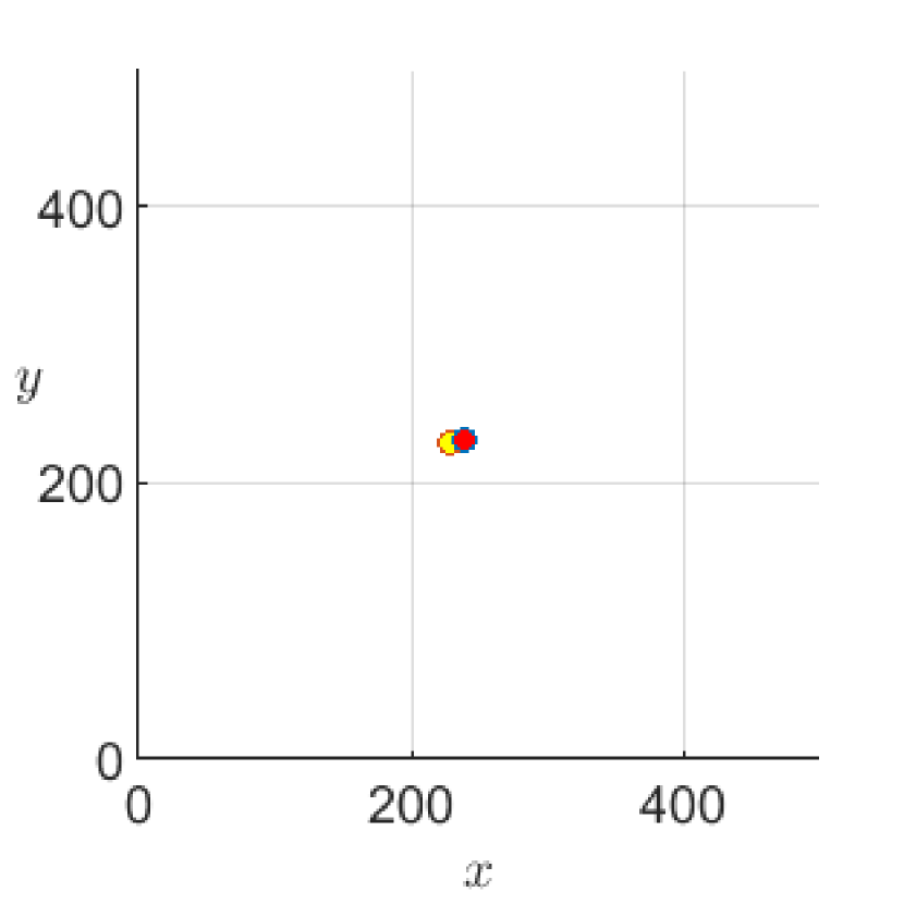
For this case, the time evolution of (1.2) is given in Figure 1. The red points and blue lines stand for the position qi(t)q_{i}(t) at t=t0t=t_{0} and trajectories for the time interval [t03,t0][t_{0}-3,t_{0}], respectively. The yellow one is for the target agent qγ(t)q_{\gamma}(t). In addition, we can check that the asymptotic complete rendezvous occurs as we proved in Theorem 2. See Figure 2. Here, the exponential function is 2e(cp+0.05)(t40)2e^{(-c_{p}+0.05)(t-40)}.

Refer to caption

(A) max1i6qi(t)qγ\max\limits_{1\leq i\leq 6}\|q_{i}(t)-q_{\gamma}\|

Refer to caption

(B) max1i6pi(t)pγ\max\limits_{1\leq i\leq 6}\|p_{i}(t)-p_{\gamma}\|

Refer to caption

(C) Logplot of (A) and (B)

Figure 2. The asymptotic complete rendezvous

For the zero extra control law, i.e. Ui=0U_{i}=0, we fix the parameters such that

σ=1,cq=4,cp=4,a=0.5.\sigma=1,~{}c_{q}=4,~{}c_{p}=4,~{}a=0.5.

The initial data of agents are randomly chosen but near the target as follows:

q1(0)=(0.8147,0.5366,0.2193),\displaystyle q_{1}(0)=(-0.8147,-0.5366,\phantom{-}0.2193), q2(0)=(0.4575,0.8843,0.0922),\displaystyle q_{2}(0)=(-0.4575,-0.8843,\phantom{-}0.0922),
q3(0)=(0.4335,0.8173,0.3794),\displaystyle q_{3}(0)=(-0.4335,-0.8173,\phantom{-}0.3794), q4(0)=(0.8645,0.2373,0.4429),\displaystyle q_{4}(0)=(-0.8645,-0.2373,\phantom{-}0.4429),
q5(0)=(0.4420,0.7998,0.4060),\displaystyle q_{5}(0)=(-0.4420,-0.7998,\phantom{-}0.4060), q6(0)=(0.4312,0.6004,0.6734),\displaystyle q_{6}(0)=(-0.4312,-0.6004,\phantom{-}0.6734),

and

p1(0)=(0.0228,0.0750,0.0987),\displaystyle p_{1}(0)=(0.0228,-0.0750,-0.0987), p2(0)=(0.2519,0.1263,0.0383),\displaystyle p_{2}(0)=(0.2519,-0.1263,\phantom{-}0.0383),
p3(0)=(0.0200,0.0169,0.0594),\displaystyle p_{3}(0)=(0.0200,\phantom{-}0.0169,\phantom{-}0.0594), p4(0)=(0.0388,0.1447,0.0017),\displaystyle p_{4}(0)=(0.0388,-0.1447,-0.0017),
p5(0)=(0.0365,0.1109,0.2583),\displaystyle p_{5}(0)=(0.0365,\phantom{-}0.1109,\phantom{-}0.2583), p6(0)=(0.0081,0.0050,0.0097).\displaystyle p_{6}(0)=(0.0081,\phantom{-}0.0050,\phantom{-}0.0097).
Refer to caption

(A) t=0t=0

Refer to caption

(B) t=1t=1

Refer to caption

(C) t=4t=4

Refer to caption

(D) t=9t=9

Refer to caption

(E) t=35t=35

Refer to caption

(F) t=90t=90

Refer to caption

(G) t=150t=150

Refer to caption

(H) t=200t=200

Figure 3. The time evolution of (1.2) with control law

The initial data for the target is given by

qγ(0)=(0.6324,0.6324,0.4472)andpγ(0)=(0.4712,0.1742,0.4199).q_{\gamma}(0)=(-0.6324,-0.6324,0.4472)\quad\text{and}\quad p_{\gamma}(0)=(0.4712,-0.1742,0.4199).

Figure 3 shows the time evolution of (1.2) without extra control law.

We can see that the maximum distance

max1i6qi(t)qγ(t)\max\limits_{1\leq i\leq 6}\|q_{i}(t)-q_{\gamma}(t)\|

between agents and the target is bounded by 2/cp2/\sqrt{c_{p}}. See Figure 4(A). Let

d(t)=max1i6qi(t)qγ(t).d(t)=\max\limits_{1\leq i\leq 6}\|q_{i}(t)-q_{\gamma}(t)\|.

Figure 4(B) displays d(t)d(t) at t=100t=100 with respect to cpc_{p}. As cpc_{p} increases, the maximum distance between agents and target decreases. Therefore, we observe that the asymptotic practical rendezvous occurs.

Refer to caption

(A) max1i6qi(t)qγ(t)\max\limits_{1\leq i\leq 6}\|q_{i}(t)-q_{\gamma}(t)\|

Refer to caption

(B) d(t)d(t) at t=100t=100

Figure 4. The asymptotic practical rendezvous

With the extra control law, we observed the asymptotic complete rendezvous in Figure 1 and Figure 2. However, if we choose the parameter cpc_{p} as zero, then the agents are not able to track the target. See Figure 5. Here, other parameters and initial data are the same as the case in Figure 1. In the absence of the velocity alignment term, the agents easily escape the sphere due to the accumulation of errors. To overcome this, as in [8], we add the following feedback term fi0f_{i}^{0} on the second equation of (1.2).

fi0=k0(qiqiqi),f_{i}^{0}=-k_{0}\Big{(}q_{i}-\frac{q_{i}}{\|q_{i}\|}\Big{)},

where k0=104k_{0}=10^{4}. From this, we conclude that the velocity alignment operator is crucial in this target tracking algorithm.

Refer to caption

(A) t=5t=5

Refer to caption

(B) t=55t=55

Refer to caption

(C) t=100t=100

Refer to caption

(D) t=200t=200

Figure 5. The time evolution of (1.2) with extra control law (6.1) and cp=0c_{p}=0

As we mentioned in Subsection 2.2, the flocking term is negligible for the target tracking problem (1.2). With the same parameters of Figure 1 and Figure 3, the numerical results of (1.2) including the rotational flocking term

j=1NψijN(Rqjqi(pj)pi),\sum_{j=1}^{N}\frac{\psi_{ij}}{N}(R_{q_{j}\to q_{i}}(p_{j})-p_{i}),

where ψij=1\psi_{ij}=1 is given in Figure 6. It is confirmed that the flocking term does not affect the results. See also Figure 7.

Refer to caption
Refer to caption
Refer to caption
Figure 6. The numerical results with flocking term and the same parameters with Figure 2
Refer to caption
Refer to caption
Figure 7. The numerical results with flocking term and the same parameters with Figure 4

Finally, we compare the target tracking problems on a sphere and flat space numerically. To compare the two cases, we impose the periodic boundary for the flat space and fix parameters such as σ=1\sigma=1, cq=5c_{q}=5, and cp=0.1c_{p}=0.1. Let

uγ=(acost,asint,a),u_{\gamma}=(a\cos t,a\sin t,a),

where a=0.5a=0.5 and ui=uγu_{i}=u_{\gamma}. Then we can observe that the complete rendezvous occurs. See Figure 8. If ui=0u_{i}=0, then we observe the practical rendezvous. See Figure 9.

Refer to caption

(A) t=0t=0

Refer to caption

(B) t=5t=5

Refer to caption

(C) t=10t=10

Refer to caption

(D) t=15t=15

Refer to caption

(E) t=40t=40

Refer to caption

(F) t=100t=100

Refer to caption

(G) t=200t=200

Refer to caption

(H) t=300t=300

Figure 8. The snapshops of complete rendezvous on flat space
Refer to caption

(A) t=0t=0

Refer to caption

(B) t=5t=5

Refer to caption

(C) t=10t=10

Refer to caption

(D) t=15t=15

Refer to caption

(E) t=40t=40

Refer to caption

(F) t=100t=100

Refer to caption

(G) t=200t=200

Refer to caption

(H) t=300t=300

Figure 9. The snapshops of practical rendezvous on flat space

7. Conclusion

In this paper, we proposed a novel model for target tracking on spherical geometry. With the target’s position, velocity, and acceleration, if the initial energy of agents is small or the bonding force between the target and each agent is larger than the one between agents, the complete rendezvous occurs. When only the information of position and velocity is known and the target’s angular velocity and its time derivative are bounded, the practical rendezvous is obtained for relatively large intra-bonding forces. The target tracking problems on 𝕊2\mathbb{S}^{2} with time delay, white noises from the observation, and measurement are also interesting topics. These issues will be discussed in our future researches.

Appendix A Properties of the admissible rotation operator

In this part, we consider admissible rotation operators on a sphere and their properties. The rotation operator appears naturally for defining the flocking on a sphere [6]. Let RR_{\cdot\rightarrow\cdot} be Rodrigues’ rotation operator given by

Rxkxi(vk)=R(xk,xi)vkR_{x_{k}\rightarrow x_{i}}(v_{k})=R(x_{k},x_{i})\cdot v_{k}

and for xkxix_{k}\neq x_{i},

R(xk,xi):=xk,xiI+xixkTxkxiT+(1xk,xi)(xk×xi|xk×xi|)(xk×xi|xk×xi|)T.\displaystyle\begin{aligned} R(x_{k},x_{i}):=\langle x_{k},x_{i}\rangle I+x_{i}x_{k}^{T}-x_{k}x_{i}^{T}+(1-\langle x_{k},x_{i}\rangle)\left(\frac{x_{k}\times x_{i}}{|x_{k}\times x_{i}|}\right)\left(\frac{x_{k}\times x_{i}}{|x_{k}\times x_{i}|}\right)^{T}.\end{aligned}

Here, xkx_{k}, xix_{i} and vjv_{j} are three dimensional column vectors. The rotation operator R{R_{\cdot\rightarrow\cdot}} has many good properties we desired or needed to be physically established and we can construct a flocking model by replacing the velocity difference term vivjv_{i}-v_{j} in the flat space to Rxjxivj(t)vi(t){R_{x_{j}\rightarrow x_{i}}}v_{j}(t)-v_{i}(t). See [6] for the details. However, there are some inconvenient points due to the presence of singularity on R{R_{\cdot\rightarrow\cdot}}. Therefore, we can naturally ask whether such alternatives can be found.

The idea to find the alternative is as follows. First, classify the properties that the rotation operators must satisfy, and find all the operators that satisfy the properties. Next, we will choose one of those operators that meets our needs. Our option will be the simplest of the possible operators. This form has various advantages. It is convenient to calculate, and it shares most of the good properties of the rotation operator R{R_{\cdot\rightarrow\cdot}} previously defined. By removing the singularity, we easily show the global-in-time existence and uniqueness of the new model in (1.2). See [6] for the existence and uniqueness of the model with R{R_{\cdot\rightarrow\cdot}}.

To construct a unit sphere model with the Newtonian equation, we need a modification of vjviv_{j}-v_{i} terms, which is the first motivation of the operators Rxjxi{R_{x_{j}\rightarrow x_{i}}} in [6]. As we compute the velocity difference between viv_{i} and vjv_{j} at the point xix_{i}, we should transform vjv_{j} into a tangential vector of the sphere at xix_{i}. We note that the typical ansatz for the flocking motion on a sphere is circle motions. In order to include circle motions along one great circle, the operator should coincide with a rotation operator in two dimensions, a (xi,xj)(x_{i},x_{j})-plane. In other words, an admissible rotation operator MM from z1z_{1} to z2z_{2} can be a 3×33\times 3 matrix such that

Mz1=z2,Mz2=2z1,z2z2z1,\displaystyle Mz_{1}=z_{2},\qquad Mz_{2}=2\langle z_{1},z_{2}\rangle z_{2}-z_{1}, (A.1a)
Mv,z2=0 for any z1,z2𝒟 and vTz1𝒟.\displaystyle\langle Mv,z_{2}\rangle=0\hbox{ for any }z_{1},z_{2}\in\mathcal{D}\hbox{ and }v\in T_{z_{1}}\mathcal{D}. (A.1b)

In the next proposition, we can prove that the admissible choices in (A.1) for the rotation operator are equivalent to the following set.

𝒜z1z2:={Pz1z2+a(z1×z2)(z1×z2)T+b(z1z1,z2z2)(z1×z2)T:a,b},\displaystyle{\mathcal{A}}_{z_{1}\rightarrow z_{2}}:=\left\{{P}_{z_{1}\rightarrow z_{2}}+a(z_{1}\times z_{2})(z_{1}\times z_{2})^{T}+b(z_{1}-\langle z_{1},z_{2}\rangle z_{2})(z_{1}\times z_{2})^{T}:a,b\in\mathbb{R}\right\}, (A.2)

where Pz1z2{P}_{z_{1}\rightarrow z_{2}} is the operator defined in (1.4).

Proposition A.1.

Suppose that unit vectors z1z_{1} and z2z_{2} are linearly independent. Then, a 3×33\times 3 matrix MM satisfies (A.1) if and only if M𝒜z1z2M\in{\mathcal{A}}_{z_{1}\rightarrow z_{2}}.

Proof.

As two vectors z1z_{1} and z2z_{2} are perpendicular to z1×z2{z_{1}\times z_{2}}, operator Pz1z2{P}_{z_{1}\rightarrow z_{2}} satisfies (A.1) from the direct computation. Note that z1×z2,zi=0\langle z_{1}\times z_{2},z_{i}\rangle=0 for i=1,2i=1,2. From this motivation, we naturally define

M:=Pz1z2+a(z1×z2)(z1×z2)T+b(z1z1,z2z2)(z1×z2)T\displaystyle M:={P}_{z_{1}\rightarrow z_{2}}+a(z_{1}\times z_{2})(z_{1}\times z_{2})^{T}+b(z_{1}-\langle z_{1},z_{2}\rangle z_{2})(z_{1}\times z_{2})^{T} (A.3)

for any a,ba,b\in\mathbb{R}. Then MM satisfies (A.1a). Also, as z2z_{2} is perpendicular to both z1×z2z_{1}\times z_{2} and (z1z1,z2z2)(z_{1}-\langle z_{1},z_{2}\rangle z_{2}), we conclude (A.1b).

Conversely, choose any 3×33\times 3 matrix MM^{\prime} satisfying (A.1). As z1z_{1} and z2z_{2} are linearly independent, {z2,z1z1,z2z2,z1×z2}\{z_{2},~{}z_{1}-\langle z_{1},z_{2}\rangle z_{2},~{}{z_{1}\times z_{2}}\} are a basis of 3\mathbb{R}^{3}. Therefore, there are a,b,ca,b,c\in\mathbb{R} such that

Mz1×z2z1×z22=a(z1×z2)+b(z1z1,z2z2)+cz2.\displaystyle M^{\prime}\frac{{z_{1}\times z_{2}}}{\|{z_{1}\times z_{2}}\|^{2}}=a(z_{1}\times z_{2})+b(z_{1}-\langle z_{1},z_{2}\rangle z_{2})+cz_{2}. (A.4)

From (A.1b) and z1×z2Tz1𝒟{z_{1}\times z_{2}}\in T_{z_{1}}\mathcal{D}, it follows that c=0c=0. Therefore, we conclude that

Mz1×z2=Mz1×z2\displaystyle M{z_{1}\times z_{2}}=M^{\prime}{z_{1}\times z_{2}}

for MM given in (A.3). On the other hand, (A.1a) show that

M(z2)=M(z2) and M(z1z1,z2z2)=M(z1z1,z2z2).\displaystyle M(z_{2})=M^{\prime}(z_{2})\quad\hbox{ and }\quad M(z_{1}-\langle z_{1},z_{2}\rangle z_{2})=M^{\prime}(z_{1}-\langle z_{1},z_{2}\rangle z_{2}). (A.5)

From (A.4) and (A.5), we obtain that M=MM=M^{\prime}. ∎

The set 𝒜z1z2{\mathcal{A}}_{z_{1}\rightarrow z_{2}} includes the rotation operators Rz1z2{R_{z_{1}\rightarrow z_{2}}} and Pz1z2{P}_{z_{1}\rightarrow z_{2}} given in [6] and (1.4), respectively. Here, if we take the following values in (A.3):

a=1z1,z2z1×z22andb=0,a=\frac{1-\langle z_{1},z_{2}\rangle}{\|{z_{1}\times z_{2}}\|^{2}}\quad\mbox{and}\quad b=0,

then the matrix coincides with Rz1z2{R_{z_{1}\rightarrow z_{2}}}, which preserves the modulus of each vectors. See Lemma 2.3 in [6]. Among several choices in the admissible set in (A.2), Pz1z2{P}_{z_{1}\rightarrow z_{2}} can be regarded as the simplest choice such that a=b=0a=b=0 in (A.2). Moreover, there is no singularity compared to the previous rotation operator R{R_{\cdot\rightarrow\cdot}}. In addition to this simplicity, the rotation operator Pz1z2{P}_{z_{1}\rightarrow z_{2}} also share the following desired transport properties.

Lemma A.2.

For z1,z2𝒟z_{1},z_{2}\in\mathcal{D}, Pz1z2{P}_{z_{1}\rightarrow z_{2}} given in (1.4) satisfies (A.1). Furthermore, we have

Pz1z2T=Pz2z1\displaystyle{P}_{z_{1}\rightarrow z_{2}}^{T}={P}_{z_{2}\rightarrow z_{1}} (A.6)

and

Pz1z2TPz1z2(z1)=z1,Pz1z2TPz1z2(z2)=z2.\displaystyle{P}_{z_{1}\rightarrow z_{2}}^{T}{P}_{z_{1}\rightarrow z_{2}}(z_{1})=z_{1},\quad{P}_{z_{1}\rightarrow z_{2}}^{T}{P}_{z_{1}\rightarrow z_{2}}(z_{2})=z_{2}.
Proof.

As two vectors z1z_{1} and z2z_{2} are perpendicular to z1×z2{z_{1}\times z_{2}}, the properties in (A.1) follow from the direct computation. Also, since the transpose is the linear operator, we have

Pz1z2T\displaystyle{P}_{z_{1}\rightarrow z_{2}}^{T} =z1,z2Iz2z1T+z1z2T,\displaystyle=\langle z_{1},z_{2}\rangle I-z_{2}z_{1}^{T}+z_{1}z_{2}^{T},

and we conclude (A.6). From (A.1) and (A.6), it holds that

Pz1z2TPz1z2(z1)=Pz1z2T(z2)=z1\displaystyle{P}_{z_{1}\rightarrow z_{2}}^{T}{P}_{z_{1}\rightarrow z_{2}}(z_{1})={P}_{z_{1}\rightarrow z_{2}}^{T}(z_{2})=z_{1}

and

Pz1z2TPz1z2(z2)=Pz1z2T(2z1,z2z2z1)=2z1,z2z1(2z1,z2z1z2)=z2.\displaystyle{P}_{z_{1}\rightarrow z_{2}}^{T}{P}_{z_{1}\rightarrow z_{2}}(z_{2})={P}_{z_{1}\rightarrow z_{2}}^{T}(2\langle z_{1},z_{2}\rangle z_{2}-z_{1})=2\langle z_{1},z_{2}\rangle z_{1}-(2\langle z_{1},z_{2}\rangle z_{1}-z_{2})=z_{2}.

While the two operators Rz1z2{R_{z_{1}\rightarrow z_{2}}} and Pz1z2{P}_{z_{1}\rightarrow z_{2}} coincide on the (z1,z2)(z_{1},z_{2})-plane from Lemma A.2, the following lemma gives us one difference between the two operators. We can show that P{{P}_{\cdot\rightarrow\cdot}} gives a map between two tangent spaces although the operator is not a bijection if z1,z2=0\langle z_{1},z_{2}\rangle=0.

Lemma A.3.

Pz1z2|Tz1𝒟{P}_{z_{1}\rightarrow z_{2}}|_{T_{z_{1}}\mathcal{D}} is a map from Tz1𝒟T_{z_{1}}\mathcal{D} to Tz2𝒟T_{z_{2}}\mathcal{D}. Furthermore, if z1,z20\langle z_{1},z_{2}\rangle\neq 0, then Pz1z2|Tz1𝒟{P}_{z_{1}\rightarrow z_{2}}|_{T_{z_{1}}\mathcal{D}} is a bijection from Tz1𝒟T_{z_{1}}\mathcal{D} to Tz2𝒟T_{z_{2}}\mathcal{D}.

Proof.

As 𝒟\mathcal{D} is a unit sphere, vTy𝒟v\in T_{y}\mathcal{D}  if and only if  v,y=0\langle v,y\rangle=0 for any y3y\in\mathbb{R}^{3}. Thus, we have

v,z1=0 for any vector vTz1𝒟.\displaystyle\langle v,z_{1}\rangle=0\quad\hbox{ for any vector }v\in T_{z_{1}}\mathcal{D}. (A.7)

From (A.1a) and (A.6), it holds that for any v3v\in\mathbb{R}^{3},

(Pz1z2v)z2=vTPz1z2Tz2=vTPz1z2rz2=vTz1=v,z1.\displaystyle({P}_{z_{1}\rightarrow z_{2}}v)\cdot z_{2}=v^{T}{P}_{z_{1}\rightarrow z_{2}}^{T}z_{2}=v^{T}{P}_{z_{1}\rightarrow z_{2}}rz_{2}=v^{T}z_{1}=\langle v,z_{1}\rangle. (A.8)

By (A.7) and (A.8), we conclude that

(Pz1z2v)z2=0 and thus Pz1z2vTz2𝒟 for any vector vTz1𝒟.\displaystyle({P}_{z_{1}\rightarrow z_{2}}v)\cdot z_{2}=0\hbox{ and thus }{P}_{z_{1}\rightarrow z_{2}}v\in T_{z_{2}}\mathcal{D}\hbox{ for any vector }v\in T_{z_{1}}\mathcal{D}.

We now assume that z1,z20\langle z_{1},z_{2}\rangle\neq 0 and show that Pz1z2|Tz1𝒟{P}_{z_{1}\rightarrow z_{2}}|_{T_{z_{1}}\mathcal{D}} is bijective between two tangent spaces. First, if z1=z2z_{1}=z_{2} or z1=z2z_{1}=-z_{2}, we get Pz1z2=I{P}_{z_{1}\rightarrow z_{2}}=I and Pz1z2=I{P}_{z_{1}\rightarrow z_{2}}=-I. If not, z1z_{1} and z2z_{2} are linearly independent. From the assumption, Pz1z2(z1×z2)=z1,z2(z1×z2){P}_{z_{1}\rightarrow z_{2}}(z_{1}\times z_{2})=\langle z_{1},z_{2}\rangle(z_{1}\times z_{2}) is a nonzero vector. Combining this with (A.1a), we conclude that Pz1z2|Tz1𝒟{P}_{z_{1}\rightarrow z_{2}}|_{T_{z_{1}}\mathcal{D}} is surjective in Tz2𝒟T_{z_{2}}\mathcal{D} and thus the determinant of Pz1z2{P}_{z_{1}\rightarrow z_{2}} is nonzero. As the inverse function of Pz1z2{P}_{z_{1}\rightarrow z_{2}} exists, we conclude that this lemma holds. ∎

References

  • [1] Bak, S., Chau, D. P., Badie, J., Corvee, E., Brémond, F., and Thonnat, M. (2012, September). Multi-target tracking by discriminative analysis on Riemannian manifold. In 2012 19th IEEE International Conference on Image Processing (pp. 1605-1608). IEEE.
  • [2] Blackman, S. S. (2004). Multiple hypothesis tracking for multiple target tracking. IEEE Aerospace and Electronic Systems Magazine, 19(1), 5-18.
  • [3] Blackman, S. S. (1986). Multiple-target tracking with radar applications. Dedham.
  • [4] Chi, D., Choi, S.-H. and Ha, S.-Y.(2014). Emergent behaviors of a holonomic particle system on a sphere. Journal of Mathematical Physics, 55, 052703.
  • [5] Choi, S.-H., Cho, J. and Ha, S.-Y.(2016). Practical quantum synchronization for the Schrödinger–Lohe system. Journal of Physics A: Mathematical and Theoretical, 49(20), 205203.
  • [6] Choi, S.-H., Kwon, D. and Seo, H. (2020). Cucker-Smale type flocking models on a sphere. arXiv preprint arXiv:2010.10693.
  • [7] Choi, S.-H., Kwon, D. and Seo, H.: Uniform position alignment estimate of a spherical flocking model with inter-particle bonding forces. arXiv preprint arXiv:2101.00791.
  • [8] Choi, S.-H., Kwon, D. and Seo, H.: Flocking formation and stabilizer of boosted cooperative control on a sphere, preprint.
  • [9] Daeipour, E., and Bar-Shalom, Y. (1995). An interacting multiple model approach for target tracking with glint noise. IEEE Transactions on Aerospace and Electronic Systems, 31(2), 706-715.
  • [10] Deghat, M., Shames, I., Anderson, B. D., and Yu, C. (2014). Localization and circumnavigation of a slowly moving target using bearing measurements. IEEE Transactions on Automatic Control, 59(8), 2182-2188.
  • [11] Olfati-Saber, R. (2006). Flocking for multi-agent dynamic systems: Algorithms and theory. IEEE Transactions on automatic control, 51(3), 401-420.
  • [12] He, T., Vicaire, P., Yan, T., Luo, L., Gu, L., Zhou, G., Stoleru, R., Cao, Q., Stankovic,J. A. and Abdelzaher, T.(2006). Achieving real-time target tracking usingwireless sensor networks. 12th IEEE Real-Time and Embedded Technology and Applications Symposium (RTAS’06). IEEE, 2006.
  • [13] Hu, J., and Hu, X. (2010). Nonlinear filtering in target tracking using cooperative mobile sensors. Automatica, 46(12), 2041-2046.
  • [14] Jia-qiang, L., Rong-hua, Z., Jin-li, C., Chun-yan, Z., and Yan-ping, Z. (2016). Target tracking algorithm based on adaptive strong tracking particle filter. IET Science, Measurement & Technology, 10(7), 704-710.
  • [15] Li, X. R., and Jilkov, V. P. (2004, August). A survey of maneuvering target tracking: approximation techniques for nonlinear filtering. In Signal and Data Processing of Small Targets 2004 (Vol. 5428, pp. 537-550). International Society for Optics and Photonics.
  • [16] Madyastha, V. K., and Caliset, A. J. (2005, June). An adaptive filtering approach to target tracking. In Proceedings of the 2005, American Control Conference, 2005. (pp. 1269-1274). IEEE.
  • [17] Oh, S., Sastry, S., and Schenato, L. (2005, April). A hierarchical multiple-target tracking algorithm for sensor networks. In Proceedings of the 2005 IEEE International Conference on Robotics and Automation (pp. 2197-2202). IEEE.
  • [18] Semnani, S. H., and Basir, O. A. (2014). Semi-flocking algorithm for motion control of mobile sensors in large-scale surveillance systems. IEEE transactions on cybernetics, 45(1), 129-137.
  • [19] Shames, I., Dasgupta, S., Fidan, B., and Anderson, B. D. (2011). Circumnavigation using distance measurements under slow drift. IEEE Transactions on Automatic Control, 57(4), 889-903.
  • [20] Sworder, D. D., Singer, P. F., Doria, D., and Hutchins, R. G. (1993). Image-enhanced estimation methods. Proceedings of the IEEE, 81(6), 797-814.
  • [21] Teschl, G.(2012). Ordinary differential equations and dynamical systems. American Mathematical Soc. 140.
  • [22] Xu, Enyang, Zhi Ding, and Soura Dasgupta. (2011). Target tracking and mobile sensor navigation in wireless sensor networks. IEEE Transactions on mobile computing 12(1), 177-186.
  • [23] Yang, Z., Shi, X., and Chen, J. (2013). Optimal coordination of mobile sensors for target tracking under additive and multiplicative noises. IEEE Transactions on Industrial Electronics, 61(7), 3459-3468.
  • [24] Yin, Guisheng, Yanbo Li, and Jing Zhang. (2008). The Research of Video Tracking System Based on Virtual Reality. International Conference on Internet Computing in Science and Engineering. IEEE.