Multi-Agent Recurrent Rendezvous Using Drive-Based Motivation
Abstract
Recent papers have introduced the Motivation Dynamics framework, which uses bifurcations to encode decision-making behavior in an autonomous mobile agent. In this paper, we consider the multi-agent extension of the Motivation Dynamics framework and show how the framework can be extended to encode persistent multi-agent rendezvous behaviors. We analytically characterize the bifurcation properties of the resulting system, and numerically show that it exhibits complex recurrent behavior suggestive of a strange attractor.
1 Introduction
Consider a group of people monitoring wildlife in a large area. Each person has a different location where they monitor the nest or den of some local animal, say a songbird. An individual will record the bird, make notes on its behavior, and otherwise gather information. Then, once sufficient information has been gathered, all members of the group rendezvous with each other to compare notes. Then, the group splits up again to gather more information. Abstractly, this is a problem of recurrent rendezvous alternating with designated tasks. In this paper we focus on developing a control scheme to automatically stabilize such a recurrent rendezvous behavior for a system of autonomous mobile robots.
The multi-agent rendezvous problem sits at the intersection of robot motion planning and distributed control. In the problem, multiple autonomous robots must coordinate and arrive at a location in space which is not predefined. There may be constraints on what an agent knows about the space or the other agents. Additional challenges such as obstacles, adversaries, or noise may be present.
The multi-agent rendezvous problem has seen significant attention in recent decades [1, 5, 14, 3], with applications such as coverage and exploration [13, 22], persistent recharging [15, 16], and simultaneous location and mapping (SLAM) [24]. Analyzing rendezvous is typically done using graph based approaches [15, 17] (where one views the agents as nodes in a communication network, and analyzes various graph metrics) and dynamical systems tools [6].
We distinguish two cases of the rendezvous problem. First is the case of one-time rendezvous, or non-recurrent rendezvous. Here the rendezvous problem is solved once the agents reach consensus. That is, if the problem begins at time , the problem is solved if there is some time when the positions of the agents have reached (or are close enough to) a point in the state space (possibly arbitrary). The second is the case of recurrent rendezvous. Here agents must always eventually rendezvous. That is, the recurrent problem is solved if for every time there exists some later time when the agents reach a common point in the state space. There is some work on recurrent rendezvous, such as addressing the issue of autonomous vehicles needing to repetitively recharge [15, 16], however most attention is given to the non-recurrent case. In this paper we focus on the recurrent case.
When designing controllers to execute repetitive tasks, one approach is for an individual agent to use a decision making model to coordinate these tasks. Here we consider a task based approach to the problem of persistent multi-agent rendezvous. Task based autonomous behavior has been widely studied [7, 8, 11]: complex behaviors are constructed from smaller, simpler tasks. Each individual task is encoded in a vector field (e.g., going to a target state is encoded as an attracting fixed point on the state space). The goal of the autonomous controller is to then coordinate these tasks to achieve said high-level behavior. Ultimately, this coordination can be framed as a form of decision making, which is a large and active area of research.
An individual in a decision making model has an action space , and state space . If and are the action and state at time we can define the history as the tuple . A policy is a map . In some cases we have a memory-less policy. That is, a policy that only depends on the current state . While we have used notation that implies discrete time, this generalizes to the continuous time case in a natural way. For our applications it will be most reasonable to consider the continuous time case, and that will be the assumption from here on.
In our task-based framework an action is choosing which of tasks to pursue. It is convenient for us to phrase our policy as an optimization problem. We consider an expanded state space where is our physical state and is our value state. The value state encodes the relative values of pursuing each of the tasks. Our policy is then to pick the action which coincides with the task with maximal value. When framing the action/policy/state system as a control system, it is useful to introduce a motivation state which tracks the current task being pursued. Here is the space of possible motivation states, and it may be discrete or continuous.
Most decision making research reduces the problem to discrete decision states: Given tasks, pick exactly one to pursue. This can be formulated mathematically. Consider a motivation vector such that iff , and otherwise. We call this the discrete motivation case. A natural extension, and one that has been of recent interest, is the continuous motivation case. The difference is that we consider the motivation vector to live on the -simplex , where . Then, following the work in [18, 20, 21], we use a pitchfork bifurcation to encode a dynamical operation analogous to the operation from the discrete case. Following [20], we term the resulting dynamical system motivation dynamics. Considering a continuous motivation state for our tasks produces interesting dynamics in the control system that are not otherwise seen in the discrete case. Moreover, it is possible to make entire system smooth, allowing for the use of smooth function analysis, as well as direct numerical integration.
The work we present here is complementary to other recent work using bifurcation theory to construct decision-making mechanisms, e.g., [10, 4, 19, 2]. In contrast to these works, here we focus not on the decision-making mechanism itself, but on connecting the mechanism to physically-embedded tasks, i.e., the requirement for the various agents to move and perform rendezvous in response to their decisions.
The main contribution of this paper is to address the persistent rendezvous problem using task-based navigation with a continuous motivation state. In the process, we develop a networked dynamical system that exhibits stable recurrent rendezvous encoded by an attractor. Concretely, our contributions are two-fold. First we develop the multi-agent extension of a control scheme originally developed in [20] and expanded upon in [23]. The scheme utilizes the so-called unfolding pitchfork bifurcation to coordinate agents with binary tasks. We then adapt this framework to the persistent rendezvous problem, and analyze the resulting dynamical system in a highly symmetric case. We derive analytical guarantees of the system behavior, and show that it achieves persistent rendezvous under appropriate conditions. In Theorem 3.7 we consider a limited form of the system and extract a closed-form critical parameter value for the breaking of system deadlock. Then, in Theorem 3.8 we view the full system, and using results from the previous theorem, we prove the existence of such critical parameter values, along with a guaranteed bound for breaking deadlock. Next, by varying parameters and (defined below), we characterize distinct regimes of behavior for the system (see Figure 1). Finally we discuss the results and provide a list of further research directions to be considered.
![[Uncaptioned image]](https://cdn.awesomepapers.org/papers/36fb410c-0cdf-4106-8714-df3b1386ea8f/consensus_regimes_1.png)
2 Preliminaries
We use the Motivation Dynamics framework [20]. Here, we extend the Motivation Dynamics framework to the -agent case. We assume that each agent has physical state and that its physical dynamics are fully actuated, i.e., that , with . We assume that each agent has two tasks, one of which is to travel to a designated location, and the other is to rendezvous with the other agents. The values associated with these two tasks for agent are encoded in The two-task assumption allows us to reduce the motivation space, , to an interval on the real line. It is convenient to consider the motivation state of an agent to live on the interval , where each extreme of the interval uniquely corresponds with one of the two tasks. Let the state of agent be denoted by , where is the agent’s physical location (or configuration), is the agent’s motivation state, and is the agent’s value state. We assume that the agent’s physical dynamics are fully-actuated, i.e., Denote as the matrix
| (1) |
where , , and .
For the time being, we will assume that the agents have two tasks, where their value dynamics are only influenced by their value state and the physical configuration of all agents. In this case agent is controlled by the closed loop, fully continuous dynamical system
| (2a) | ||||
| (2b) | ||||
| (2c) | ||||
where . Compactly we have
| (3) |
and in matrix form
| (4) |
We will also denote the dynamics of the matrices by , , .
2.1 Rendezvous with Designated Tasks
By convention we will have task 1 be the designated task of a given agent, and task 2 will be rendezvous. We choose point visitation as the designated task. We have
and , where is the designated point for agent to visit.
For the rendezvous task we choose navigation to the centroid. We set
which gives
Thus our first task looks like navigation to a designated point, and our second task looks like navigation to the centroid of the other agents.
3 The Symmetric Case
Assuming agents and , denote as the rotation matrix given by
| (5) |
We set the designated task locations as , where (i.e. symmetrically distributed points on the unit circle). At this point it is prudent to make the change of coordinates . Denoting the transformed matrix by , this results in
and
Moreover, we will consider symmetric time scales for the motivation and value dynamics. That is, we set and for all . Let us set and
Then we may compactly represent our symmetric-case system by the dynamical equation
| (6) |
The fact that this is the symmetric case allows us to utilize a group invariance of the system. First we note that following definition of equivariance for a map.
Definition 3.1.
Consider a map and a group with a well defined group action on elements . We say is equivariant under if for all and we have that
| (7) |
With equivariance in mind, now we establish a symmetry group for the dynamics (6).
Lemma 3.2.
Let be the cyclical group generated by the permutation (i.e. the “shift-by-one” permutation on elements). Let act on a matrix by permuting the columns of in the same way. Then we have that the mapping given in (6) is equivariant under for .
Proof.
Let represent the shift-by-one group action described above. Since generates it suffices to prove that
Let map the -th column of to . We have
and
Thus we must show that
One notes that , and thus . Then by re-indexing the sum we may write
This gives us . For it suffices to show . This follows by applying the same argument as the one given above for . Finally, one can see by inspection that . Thus we have that
Definition 3.3.
Consider a vector space with a well defined group action for elements of a group . We define the fixed point subspace of a subgroup by
| (8) |
We note that the fixed point subspace of is the one generated by matrices with all columns the same (i.e. ). We will refer to this subspace as the symmetric subspace. We will see later that said subspace possesses some very interesting properties.
3.1 Deadlock
The symmetric case displays many interesting behaviors for different parameter regimes, and some of these boundaries between regimes admit direct analysis. One such boundary is that of the deadlock case.
Definition 3.4.
We define deadlock as an equilibrium point of the system (6) such that is asymptotically stable with for all . (That is, all motivation variables are in a state of “indecision”.)
Indeed, if we search for deadlock on the symmetric subspace, we find a candidate equilibrium.
Lemma 3.5.
Let and consider . There is a potential deadlock equilibrium point on the symmetric subspace of (6) which we will denote , given by
| (9) |
where solves
| (10) |
Proof.
We are considering the symmetry subspace, and so set . In order to be a deadlock equilibrium, by Definition 3.4. Thus, we must have that . Moreover, we have that and . Substituting both into will give the cubic in (10). Back substituting will give the equilibrium values for and .
We must verify that there is exactly one root of (10) in the interval . If we input into the cubic we get respectively. We see that for there are three consecutive changes in sign of the cubic. This implies that the three roots of the cubic are all real, and lie in the intervals , , and . Roots which are greater than 1 and less than 0 will invalidate the assumption. Thus we must take the root in .
A detailed numerical search suggests that the deadlock equilibrium described in Lemma 3.5 is unique. On the basis of this numerical evidence we make the following claim.
Claim 3.6.
Let and let be the deadlock equilibrium defined in Lemma 3.5. Then is the unique equilibrium on the symmetry subspace.
To study the stability of our system we must still consider a Jacobian matrix that is . To get a better sense of the structure of the Jacobian, and how we might determine stability conditions, we will first consider the dynamics in the singularly perturbed limit of .
3.1.1 The Limit
We split our system, denoting as our slow manifold variables, and the value state as our fast manifold variable. If we then take the limit we have that
This results in the slow manifold system
| (11a) | ||||
| (11b) | ||||
We will compactly represent the system by
| (12) |
and we denote the corresponding deadlock point for the reduced system by
| (13) |
where and are still the same as in (9). In Appendix A we derive that the Jacobian can be represented compactly, and that by (24) we may write the characteristic polynomial as
| (14) |
This leads us to establish our first result
Theorem 3.7.
Proof.
From Lemma A.6, we have a compact form for the characteristic polynomial given by
where and are given in the statement of Theorem A.6. We note that both and are cubic in . Thus, one can write closed-form expressions for their roots. The expression for the roots of is very complicated, and does not admit direct analysis of the critical value for bifurcation. However, factors nicely across . Specifically, it may be written as
where for are the task function values at the deadlock point. Direct computation of the roots gives
If we can show that
then we can guarantee that have negative real parts for . Noting that can be factored from the expression above, it suffices to show
which is the case, as for and (this can be checked by looking for sign switches in the left-hand-side of (10) on the interval ).
Next we must show that the eigenvalues are complex, i.e.
for . It suffices to show
This once again holds due to the fact that for and .
It remains to show the non-tangency condition of our roots, i.e., that the roots pass through the imaginary axis. The real part of the eigenvalues is given by , so the derivative with respect to is . This is positive since .
3.1.2 The case of finite
It is possible to derive an explicit form for the characteristic polynomial of the relaxed system, but that polynomial would still be of degree 5, and in general would require numerical computations to find the roots. Indeed, given a fixed value of , we can numerically approximate the deadlock-breaking value of , and vice versa. The results of such a computation are shown in Figure 2. In place of deriving an exact form for the characteristic polynomial, we prove a lower bound on that guarantees deadlock-breaking.
Theorem 3.8.
Proof.
By Lemma B.4 we have that
The trace of a matrix is the sum of the eigenvalues, thus if the trace has positive real part there mus be at least one eigenvalue with positive real part. Setting and solving for gives the desired lower bound.
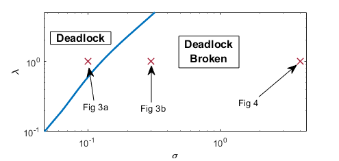
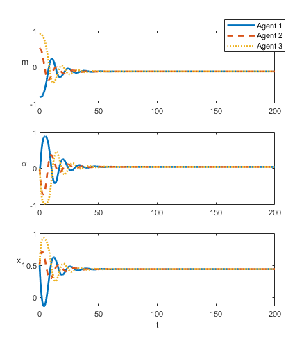
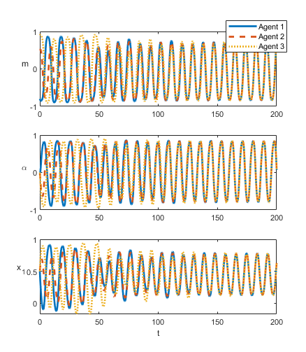
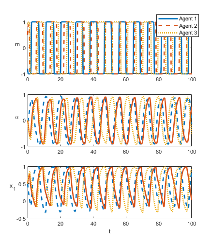
As a demonstration we have included two examples of a subset of the state trajectories under deadlock and non-deadlock in Figure 3. We track the , and states and we plot all three agents together at once. Here , which is the normalized difference between value states.
3.2 Syncronicity and Asynchronicity
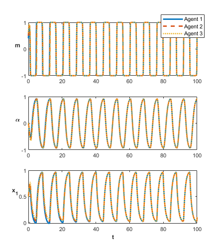
When we consider , as given in (16), and finite there are interesting dynamical regimes that emerge. Specifically, the system produces both synchronous and asynchronous rendezvous, dependent on initial conditions and parameter regimes. At this point, further direct analysis of the system becomes far less tractable, and yields very little information. Instead we will investigate these regimes numerically. For the remainder of this section we will consider the case , as it is the simplest case that still experiences rich behavior.
Once we are in the deadlock broken regime (See Figure 2) the system can experience either synchronous or asynchronous rendezvous (See Figure 4). Synchronicity for fixed and depends only on the initial conditions of the system. We should stress the system still experiences recurrent rendezvous, even in the asynchronous case. One way to see this is to consider the average distance to the centroid across all agents as it varies over time. We define the rendezvous metric by
| (17) |
or for the transformed variable we have
| (18) |
We plot two examples in Figure 5.
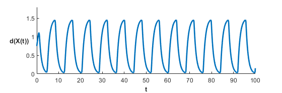
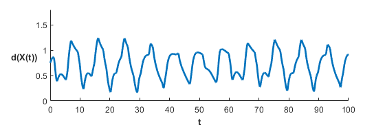
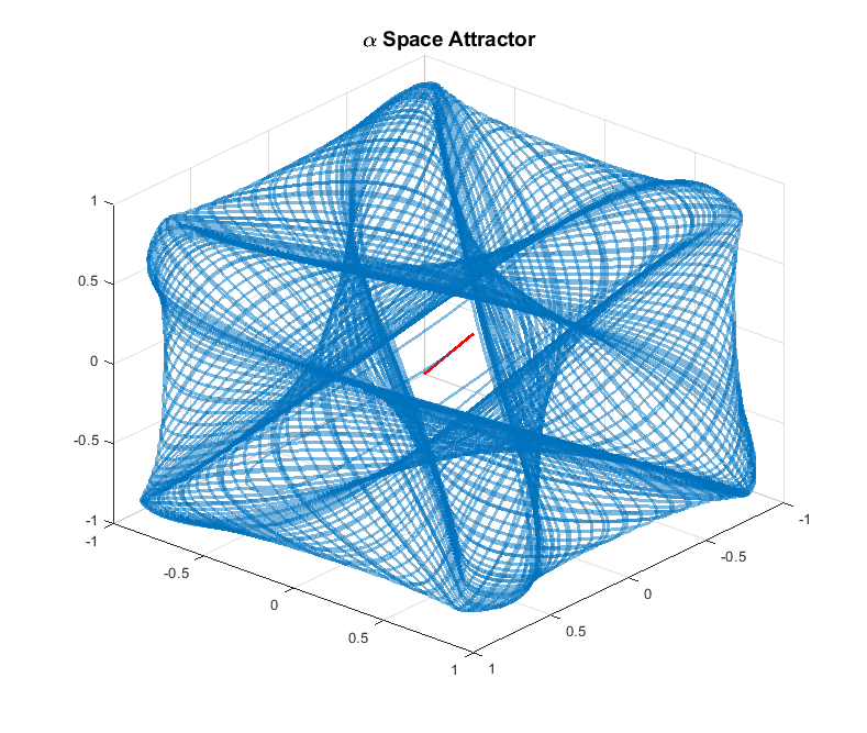
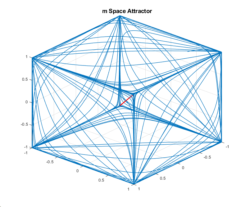
Despite not performing as well as the synchronous case, the asynchronous case shows that the agents repetitively get close to one another. Under reasonably relaxed constraints this constitutes recurrent rendezvous. In fact, numerical evidence supports that there is an attractor of the system on which the asynchronous orbits live. The attractor itself is 15 dimensional, and so we can only plot slices of the state space. We consider the space of the 3 agent system, recalling that , and the space. Plotting trajectories in both spaces yields Figure 6.
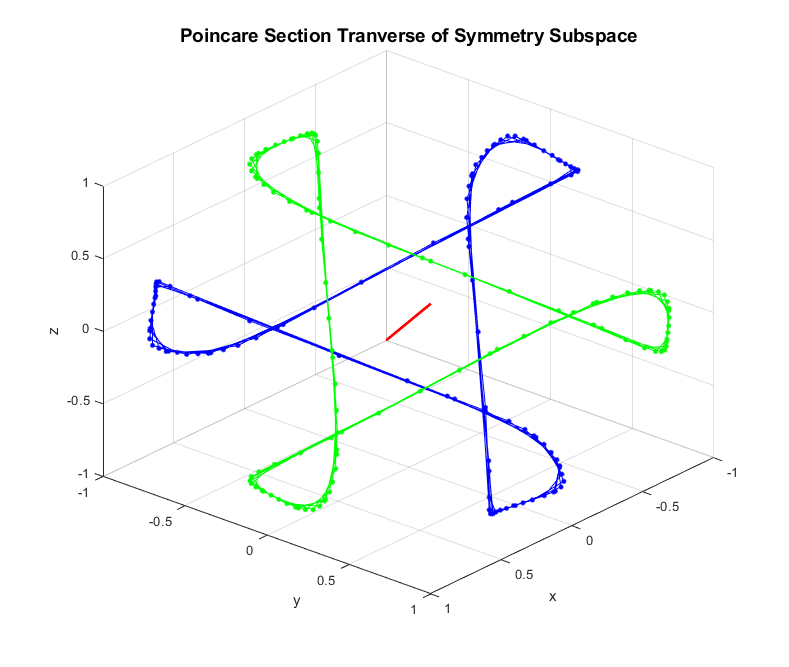
We can further characterize this attractor by taking a Poincaré section in the space. Consider the vector . We construct our section by tracking when , i.e. when the trajectory punctures the plane defined by . In addition, if we track the sign change we can see that two limit cycles emerge in the section. Let indicate the -th point in time such that . If we plot the even and odd indices separately, i.e. plot and for , we see that two limit cycles emerge in the Poincaré section (See Figure 7). These limit cycles further support the claim that the orbits are living on an attractor.
This attractor leads us to make the following claim:
Claim 3.9.
The system (6) has an attractor whose characteristics depend on the parameters .
Moreover, there exists a region of the parameter space such that is not on the synchronous manifold, and is not a fixed point.
This allows us to postulate a theorem.
Theorem 3.10.
Proof.
An attractor of a dynamical system has two necessary properties: (1) is forward invariant, i.e. any trajectory starting in stays in . (2) There is no proper subset of which has this property.
Properties (1) and (2) imply given any , any point , and any trajectory such that , there is always a point in time such that . If no such point in time existed, then we could define the -ball centered on by , and the set would satisfy property (1), which would directly contradict property (2).
Our claim in Theorem 3.10 then follows from the continuity of the rendezvous metric : Given , there exists such that if , continuity of implies that . By the preceding argument, such times must exist.
The idea here is that if the orbit (which lives on this attractor) produces a small value for the rendezvous metric, then there is a future time when the same orbit will pass close enough to the same point to produce a rendezvous metric that is sufficiently close to .
4 Discussion
In this paper, we have shown how the motivation dynamics architecture and associated results introduced in [20] can be extended to the multi-agent case. In particular, we have demonstrated the feasibility of using the unfolding pitchfork decision-making mechanism to coordinate recurrent rendezvous tasks between autonomous agents. Moreover, we have shown that the parameters of the multi-agent system (6) can be chosen in such a way as to guarantee that the system does not reach a deadlock state, and that there will always eventually be a rendezvous event. In the language of formal methods [12], our system satisfies the following specification: always ((eventually rendezvous) and (eventually visit designated location)). The connection between the structure of the dynamical system and the discrete specification that it satisfies is beyond the scope of this paper, but is of great interest for future work.
Several interesting research questions follow from the results of this paper. First, in the problem as it is presented in this paper, each agent has full knowledge of the others’ positions. In other words, the communication graph is complete and communication is uncorrupted by noise or delays. The results presented in this paper could naturally be generalized to the case of an incomplete but connected communications graph, or the cases where communication among agents is corrupted by stochastic noise or communication delays. These generalizations should be feasible given standard tools from the distributed consensus literature.
Second, the agents’ tasks may be more subtle than the tasks considered here, where each agent has two tasks: exactly one designated point-attractor task and one rendezvous task where the agents must precisely rendezvous at a point. If approximate rendezvous, e.g., to a neighborhood, is acceptable, what further results might be possible? In the case that there are point-attractor tasks and agents, how can the system automatically distribute these tasks among the agents?
Third, there is a fundamental mathematical question of characterizing the attractor whose existence we postulate in Claim 3.9. It is likely that symmetric bifurcation theory [9] will provide a set of tools to enable this analysis. Answering these questions will push forward knowledge of how the unfolding pitchfork can be used to coordinate high-level autonomous behaviors.
References
- [1] S. Alpern. The rendezvous search problem. SIAM Journal on Control and Optimization, 33(3):673–683, 1995.
- [2] A. Bizyaeva, T. Sorochkin, A. Franci, and N. E. Leonard. Control of agreement and disagreement cascades with distributed inputs, 2021.
- [3] D. V. Dimarogonas and K. J. Kyriakopoulos. On the rendezvous problem for multiple nonholonomic agents. IEEE Transactions on automatic control, 52(5):916–922, 2007.
- [4] A. Franci, M. Golubitsky, and N. E. Leonard. The dynamics of multi-agent multi-option decision making. arXiv:1909.05765, 2019.
- [5] B. A. Francis and M. Maggiore. Flocking and rendezvous in distributed robotics. Springer, 2016.
- [6] P. Friudenberg and S. Koziol. Mobile robot rendezvous using potential fields combined with parallel navigation. IEEE Access, 6:16948–16957, 2018.
- [7] C. R. Garrett, R. Chitnis, R. Holladay, B. Kim, T. Silver, L. P. Kaelbling, and T. Lozano-Pérez. Integrated task and motion planning. Annual review of control, robotics, and autonomous systems, 4:265–293, 2021.
- [8] M. Ghallab, D. Nau, and P. Traverso. Automated planning and acting. Cambridge University Press, 2016.
- [9] M. Golubitsky, I. Stewart, and D. G. Schaeffer. Singularities and groups in bifurcation theory: Vol. II. Number 69 in Applied Mathematical Sciences. Springer-Verlag, New York, 1988.
- [10] R. Gray, A. Franci, V. Srivastava, and N. E. Leonard. Multi-agent decision-making dynamics inspired by honeybees. IEEE Transactions on Control of Network Systems, 5(2):793–806, 2018.
- [11] E. Karpas and D. Magazzeni. Automated planning for robotics. Annual Review of Control, Robotics, and Autonomous Systems, 3:417–439, 2020.
- [12] H. Kress-Gazit, M. Lahijanian, and V. Raman. Synthesis for Robots: Guarantees and Feedback for Robot Behavior. Annual Review of Control, Robotics, and Autonomous Systems, 1(1):211–236, 2018.
- [13] B. Li, B. Moridian, and N. Mahmoudian. Underwater multi-robot persistent area coverage mission planning. In OCEANS 2016 MTS/IEEE Monterey, pages 1–6. IEEE, 2016.
- [14] J. Lin, A. Morse, and B. Anderson. The multi-agent rendezvous problem. an extended summary. In Cooperative Control, pages 257–289. Springer, 2005.
- [15] N. Mathew, S. L. Smith, and S. L. Waslander. A graph-based approach to multi-robot rendezvous for recharging in persistent tasks. In 2013 IEEE International Conference on Robotics and Automation, pages 3497–3502. IEEE, 2013.
- [16] N. Mathew, S. L. Smith, and S. L. Waslander. Multirobot rendezvous planning for recharging in persistent tasks. IEEE Transactions on Robotics, 31(1):128–142, 2015.
- [17] M. Meghjani and G. Dudek. Multi-robot exploration and rendezvous on graphs. In 2012 IEEE/RSJ International Conference on Intelligent Robots and Systems, pages 5270–5276. IEEE, 2012.
- [18] D. Pais, P. M. Hogan, T. Schlegel, N. R. Franks, N. E. Leonard, and J. A. Marshall. A mechanism for value-sensitive decision-making. PloS one, 8(9):e73216, 2013.
- [19] P. Reverdy. Dynamical, value-based decision making among options, 2020.
- [20] P. B. Reverdy and D. E. Koditschek. A dynamical system for prioritizing and coordinating motivations. SIAM Journal on Applied Dynamical Systems, 17(2):1683–1715, 2018.
- [21] P. B. Reverdy, V. Vasilopoulos, and D. E. Koditschek. Motivation dynamics for autonomous composition of navigation tasks. IEEE Transactions on Robotics, 2021.
- [22] N. Roy and G. Dudek. Collaborative robot exploration and rendezvous: Algorithms, performance bounds and observations. Autonomous Robots, 11(2):117–136, 2001.
- [23] C. Thompson and P. Reverdy. Drive-based motivation for coordination of limit cycle behaviors. In 2019 IEEE 58th Conference on Decision and Control (CDC), pages 244–249. IEEE, 2019.
- [24] X. S. Zhou and S. I. Roumeliotis. Multi-robot slam with unknown initial correspondence: The robot rendezvous case. In 2006 IEEE/RSJ international conference on intelligent robots and systems, pages 1785–1792. IEEE, 2006.
Appendix A Jacobian in Limit
In this appendix, we compute the Jacobian for our system (6) in the singular limit . We also derive an expression for its characteristic polynomial.
Lemma A.1.
Proof.
Direct computation.
A.1 Computation of Characteristic Polynomial of
First we state a lemma which allows us to compactly represent the Jacobian of (12) at the equilibrium point.
Lemma A.2.
Proof.
Observe that . Then have that
Thus it follows that
We can compute the characteristic polynomial by using the representation given in (22) and the Matrix Determinant Lemma, which we will state here without proof.
Lemma A.3.
Let be an invertible matrix, and let and be matrices. Then
| (23) |
With this we may reduce the determinant of to the product of determinants of matrices.
Lemma A.4.
Let and consider . Let be defined the same as in Lemma A.2. Then we may write the characteristic polynomial of as
| (24) |
where is given by
Proof.
We have that
The second equality in the derivation comes from the Matrix Determinant Lemma, and the final equality comes from the fact that the determinant of an matrix is -linear in the rows of the matrix and that is all 0 below the second row.
Before computing the characteristic polynomial we need to evaluate the expression . To do this we need the following lemma.
Lemma A.5.
Let and consider . Define to be the same as in (5). Then we have
| (25) |
Proof.
Denote . We have that
We also have that
This comes from the fact that the sum of roots of unity is 0. That is
Thus
Similarly one can show that
Thus we have that
Now we are in a place to compute the characteristic polynomial.
Lemma A.6.
The characteristic polynomial of is given by
| (26) |
where
and
with
Proof.
The adjugate of has the form
where , , and are given as in the theorem above. The expressions for and are not necessary, as one can compute
where
Applying Lemma A.5 gives us .
Now note that is precisely . If we combine these derivations with the form of given in (24) we arrive at the desired expression:
Appendix B Jacobian for finite
In this appendix we consider the full system (6). Using similar procedure as in Appendix A we a simplified expression for the characteristic polynomial and trace of the Jacobian of (6) at the equilibriup point (9).
Lemma B.1.
Proof.
Direct computation.
B.1 Computation of Characteristic Polynomial of
Lemma B.2.
Proof.
Observe that . Then have that
Thus it follows that
Lemma B.3.
Let and consider . Let be defined as in Lemma B.2. Then we may write the characteristic polynomial of as
| (31) |
where is given by
B.2 Trace of
Lemma B.4.
The trace of is given by
| (32) |
Proof.
This follows from direct computation using (27) and .