MTC: Multiresolution Tensor Completion from Partial and Coarse Observations
Abstract.
Existing tensor completion formulation mostly relies on partial observations from a single tensor. However, tensors extracted from real-world data are often more complex due to: (i) Partial observation: Only a small subset (e.g., 5%) of tensor elements are available. (ii) Coarse observation: Some tensor modes only present coarse and aggregated patterns (e.g., monthly summary instead of daily reports). In this paper, we are given a subset of the tensor and some aggregated/coarse observations (along one or more modes) and seek to recover the original fine-granular tensor with low-rank factorization. We formulate a coupled tensor completion problem and propose an efficient Multi-resolution Tensor Completion (MTC) model to solve the problem. Our MTC model explores tensor mode properties and leverages the hierarchy of resolutions to recursively initialize an optimization setup, and optimizes on the coupled system using alternating least squares. MTC ensures low computational and space complexity. We evaluate our model on two COVID-19 related spatio-temporal tensors. The experiments show that MTC could provide 65.20% and 75.79% percentage of fitness (PoF) in tensor completion with only 5% fine granular observations, which is 27.96% relative improvement over the best baseline. To evaluate the learned low-rank factors, we also design a tensor prediction task for daily and cumulative disease case predictions, where MTC achieves 50% in PoF and 30% relative improvements over the best baseline.
1. Introduction
Tensor completion is about estimating missing elements of multi-dimensional higher-order data (the dimensions of tensors are usually called “mode”s). The CANDECOMP/PARAFAC (CP) and Tucker factorization approaches are commonly used for this data denois- ing and completion task, with applications ranging from image restoration (Liu et al., 2012; Xu and Yin, 2013) to healthcare data completion (Acar et al., 2011a; Wang et al., 2015), recommendation systems (Song et al., 2017), link prediction (Lacroix et al., 2018), image fusion (Borsoi et al., 2020) and spatio-temporal prediction (Araujo et al., 2017; Kargas et al., 2021).
In many real-world tensor data, missing values and observed data have unique characteristics:
Partial observations: Real-world tensor data has many missing values (only a small subset of the elements are available). This is a common assumption in most tensor completion works (Liu et al., 2012; Acar et al., 2011a). Many existing works estimate the missing elements purely based on data statistics (Hong et al., 2020) by low-rank CP or Tucker model, while some also consider auxiliary domain knowledge (Lacroix et al., 2018; Wang et al., 2015).
Coarse observations: In many applications, tensor data is available at multiple granularity. For example, a location mode can be at zipcode, county, or state level, while a time mode can be at daily, weekly, or monthly level. Coarse-granular tensors are often fully available, while fine-granular tensors are usually incomplete with many missing elements. Few works (Almutairi et al., 2021, 2020) leverage the existing coarse level information to enhance tensor completion.
Motivating example: Given (i) partial observations: a small subset (e.g., 5%) of a fine-granular location by disease by time tensor, where each tensor element is the disease counts (by ICD-10 code111A disease can be represented with different coding standards: For example, International Classification of Disease version-10 (ICD-10) is a fine-granular code with over 100K dimensions. And Clinical Classification Software for diagnosis codes (CCS) is a coarse-granular code with O(100) dimensions.) in a geographical location (by anonymous location identifier) at a particular time (by date); (ii) coarse observations: two coarse-granular tensors at state by ICD-10 by date level and location by CCS by date level, respectively. The problem is how to recover the fine-granular location identifier by ICD-10 by date tensor based on this partial and coarse information, where the mode aggregation mechanism is sometimes unknown, especially in healthcare (Park and Ghosh, 2014).
To capture the data characteristics, we identify the following technical challenges:
-
•
Challenge in partial and coarse data fusion. While heterogeneous information could compensate with each other and serve as potential supplements, it is challenging to combine different sources in a compact tensor factorization objective.
-
•
Challenge in computational efficiency and accuracy. With the increasing data volume and multidimensional structures, it becomes challenging to choose an accurate model initialization and a fast optimization kernel.
To address these challenges, we propose a Multiresolution Tensor Completion (MTC) method with the following contributions.
-
•
MTC fuses both partial and coarse data into Frobenius norm based formulation, which is computationally efficient to deal with as they present a generic coupled-ALS form.
-
•
MTC enables an effective initialization for model optimization to improve model efficiency and accuracy. We pack multiple linear equations into one joint normal equation during optimization and propose an ALS-based solver.
We evaluate MTC on a spatio-temporal disease dataset and a public COVID keyword searching dataset. Extensive experiments demonstrate that for tensors with only 5% observed elements, MTC could provide 65.20% and 75.79% percentage of fitness (PoF) in the completion task, which shows relative improvement over the best baseline by 27.96%. We also design a tensor prediction task to evaluate the learned factors, where our model reaches nearly 50% PoF in disease prediction and outperforms the baselines by 30%.
2. Related Work on Tensors
2.1. Low-rank Tensor Completion
Tensor completion (or tensor imputation) benefits various applications, which is usually considered a byproduct when dealing with missing data during the decomposition (Song et al., 2019). The low-rank hypothesis (Larsen and Kolda, 2020) is often introduced to address the under-determined problem. Existing tensor completion works are mostly based on its partial (Acar et al., 2011a; Liu et al., 2012) or coarsely (Almutairi et al., 2020, 2021) aggregated data. Many works have employed augmented loss functions based on statistical models, such as Wasserstein distance (Afshar et al., 2021), missing values (Huang et al., 2020), noise statistics (e.g., distribution, mean or max value) (Barak and Moitra, 2016) or the aggregation patterns (Yin et al., 2019). Others have utilized other auxiliary domain knowledges, such as within-mode regularization (Kargas et al., 2021; Wang et al., 2015), -norms (Lacroix et al., 2018), pairwise constraints (Wang et al., 2015). Among which, a line of coupled matrix/tensor factorization (Almutairi et al., 2020; Araujo et al., 2017; Bahargam and Papalexakis, 2018; Huang et al., 2020; Borsoi et al., 2020) is related to our setting. One of the most noticeable works is coupled matrix and tensor factorization (CMTF) proposed by Acar. et al. (Acar et al., 2011b), where a common factor is shared between a tensor and an auxiliary matrix. Another close work (Almutairi et al., 2021) recovered the tensor from only aggregated information.
However, few works combine both the partial and coarse data by a coupled formulation. This paper fills in the gap and leverages both the partial and coarse information.
2.2. Multi-scale and Randomized Methods
With the rapid growth in data volume, multi-scale and randomized tensor methods become increasingly important for higher-order structures to boost efficiency and scalability (Larsen and Kolda, 2020; Özdemir et al., 2016).
Multi-scale methods can interpolate from low-resolution to high-resolution (Schifanella et al., 2014; Sterck and Miller, 2013; Park et al., 2020) or operate first on one part of the tensor and then progressively generalize to the whole tensor (Song et al., 2017). For example, Schifanella et al. (Schifanella et al., 2014) exploits extra domain knowledge and develops a multiresolution method to improve CP and Tucker decomposition. Song et al. (Song et al., 2017) imputes the tensor from a small corner and gradually increases on all modes by multi-aspect streaming.
The randomized methods are largely based on sampling, which accelerate the computation of over-determined least square problem (Larsen and Kolda, 2020) in ALS for dense (Ailon and Chazelle, 2006) and sparse (Eshragh et al., 2019) tensors by effective strategies, such as Fast Johnson-Lindenstrauss Transform (FJLT) (Ailon and Chazelle, 2006), leverage-based sampling (Eshragh et al., 2019) and tensor sketching.
Unlike previous methods, our model does not require a domain-specific mode hierarchy. Our multiresolution factorization relies on a heuristic mode sampling technique (mode is continuous or categorical), which is proposed to initialize the optimization phase such that fewer iterations would be needed in high resolution. Also, we consider a more challenging coupled factorization problem.
3. Preliminary
3.1. Notations
We use plain letters for scalar, such as or , boldface uppercase letters for matrices, e.g., , and Euler script letter for tensors and sets, e.g., . Tensors are multidimensional arrays indexed by three or more indices (modes). For example, an -th order tensor is an -dimensional array of size , where is the element at the -th position. For matrices, and are the -th column and row, and is for the -th element. Indices typically start from , e.g., is the first row of the matrix. In this paper, we work with a three-order tensor for simplicity, while our method could also be applied to higher-order tensors.
3.1.1. CANDECOMP/PARAFAC (CP) Decomposition.
One of the common compression methods for tensors is CP decomposition (Hitchcock, 1927; Carroll and Chang, 1970), which approximates a tensor by multiple rank-one components. For example, let be an arbitrary -mode tensor of CP rank , it can be expressed exactly by three factor matrices as
| (1) |
where is the vector outer product, and the double bracket notation is the Kruskal operator.
3.1.2. Mode Product.
For the same tensor , a coarse observation is given by conducting a tensor mode product with an aggregation matrix (for example, on the first mode), , where ,
| (2) |
where we use superscripts, e.g., , to denote the aggregated tensor. Other tensor background may be found in Appendix. We organize the symbols in Table 1.
| Symbols | Descriptions |
|---|---|
| tensor CP rank | |
| , | tensor Khatri-Rao/Hadamard product |
| tensor Kruskal operator | |
| the set of coarse tensors | |
| known/unknown/full aggregation matrix set | |
| aggregation matrices | |
| the original/interim/reconstructed tensor | |
| , | two coarse observation tensors |
| tensor unfoldings/matricizations | |
| tensor mask | |
| factor matrices | |
| auxiliary factor matrices | |
| entity or index set at resolution | |
| initializations for the factors |
3.2. Problem Definition
Problem 1 (Tensor Completion with Partial and Coarse Observations).
For an unknown tensor , we are given
-
•
a partial observation , parameterized by mask ;
-
•
a set of known aggregation matrices , each column of is one-hot;
-
•
a set of coarse tensors . For example, an coarse tensor aggregated on both the first and the second mode can be written as .
The problem is to find low-rank CP factors , such that the following (Frobenius norm based) loss is minimized,
| (3) | , |
where is the set of unknown aggregation matrices, enumerates the index of , and contains the weights that specify the importance of each coarse tensor. We separate the knowns and unknowns (to estimate) by semicolon “;”. Note that, the same mode cannot be aggregated in all coarse tensors.
3.3. A Motivating Example
As an example, we use the aforementioned COVID disease tensor to motivate our application. For an unknown location identifier by ICD-10 by date tensor , we are given
-
•
a partial observation , parametrized by mask ;
-
•
a coarse state by ICD-10 by date tensor, , where (satisfying with an unknown , since we have no knowledge on the mapping from anonymized location identifier to state);
-
•
a coarse location identifier by CCS by date tensor, , where and it satisfies with known ICD-10 to CCS mapping .
We seek to find low-rank CP factors , such that the loss is minimized over parameters (),
| (4) |
w.l.o.g., we use this example to introduce our methodology.
3.4. Solution Outline
3.4.1. Coupled Tensor Decomposition.
To address the above objective, we consider to successively approximate the low-rank completion problem by coupled tensor decomposition. We first introduce two transformations and reformulate the objective into a coupled decomposition form:
-
•
Parameter replacement. We replace and as two new auxiliary factor matrices and add extra constrains later since and are related by a known (but is unknown, we does not consider the constraint for and ).
-
•
Interim Tensor. For the first term in Equation (3.3), we construct an interim tensor from an expectation-maximization (EM) (Acar et al., 2011a) approach,
(5) where are the learned factors at the -th iteration. The reconstruction is expensive for large tensors. However, we do not need to compute it explicitly. In Section 5, we introduce a way to use the implicit form.
Afterwards, the objective in Equation (3.3) is approximated by a coupled tensor decomposition form (at the -th iteration),
| (6) | , |
with constraint and the interim tensor ,
| (7) |
Now, our goal turns into optimizing a coupled decomposition problem with five shared factors, among which are our focus.
3.4.2. Optimization Idea.
As a solution, we adopt a multiresolution strategy, as in Figure 1, which leverages a hierarchy of resolution to perform the coupled optimization effectively. The multiresolution factorization part (in Section 4) serves as the outer loop of our solution. At each resolution, we derive a joint normal equation for each factor and develop an efficient ALS-based solver (in Section 5) to handle multiple linear systems simultaneously.

4. Multiresolution Factorization
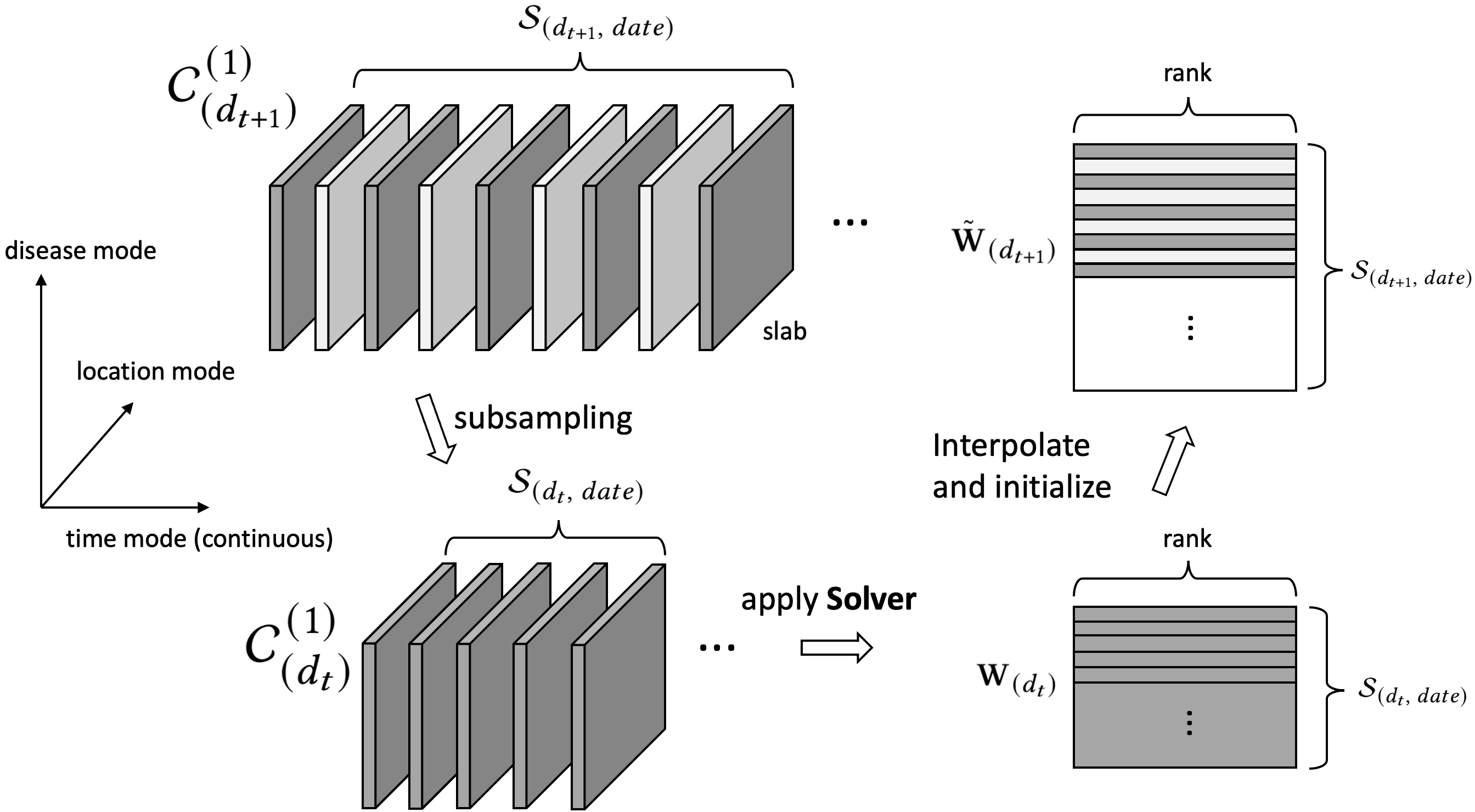
Let us denote the resolution hierarchy as , where is the highest resolution (i.e., original tensors). The multiple resolutions are computed via recursive subsampling along three tensor modes simultaneously. The underlying ideas of the multiresolution factorization are: (i) to subsample high-resolution information into low resolution and solve a low-resolution problem; (ii) to then interpolate the low-resolution solution factors for initializing the high-resolution problem, such that fewer iterations are needed in high resolution.
4.1. High () to Low () Resolution
Assume that is a generic notation for high resolution and is for the neighboring low resolution, we use subscript-parenthesis notation, e.g., to denote the entities at each resolution.
Objective at . The goal is to find optimal factor matrices: , , , , , such that they minimize the loss at (the form could refer to Equation (6)),
In the following, we conceptulize the solution to the objective.
-
(1)
Subsampling: We first subsample all accessible information (tensors and the known aggregation matrices) from to at once,
(8) . -
(2)
Solve the objective at : Next, we solve the -problem recursively and obtain smaller factor matrices (, , , ,), where the -objective can be similarly written as
(9) the interim tensor is calculated by
(10) and the resolution constraint is .
-
(3)
Interpolation: Then, we interpolate the solutions to initialize the problem. More precisely, four factor matrices are obtained by interpolation:
(11) (12) . And one is calculated by the known aggregation matrix according to the constraint:
(13) -
(4)
Optimization at : With the initialized factor matrices, we finally can apply our optimization algorithm recursively on the objective to improve the factors.
These four steps are the key to the paper. The multiresolution factorization is conducted by recursively applying four steps within Step (2). In this section, Step (1) and (3) are of our focus, while we will specify Step (4) in Section 5. The subsampling and interpolation are closely related, and we elucidate them below.
4.2. Resolution Transition from to
In our example, three modes are presented with -specific mode sizes: (i) location mode: anonymized location identifier , state ; (ii) disease mode: ICD-10 , CCS ; (iii) time mode: date . To make it clear, we use the term aspect to indicate a tensor mode or its projection/aggregation at a coarse granularity.
In total, we have three modes in our problem and five different aspects, corresponding to five factors. We call a mode with two aspects an aggregated mode and a mode with one aspect as an single mode. For example, the location and disease modes are aggregated modes, and the time mode is a single mode. Because location mode can be at zipcode or state aspect; disease mode can be at ICD-10 aspect (fine-granular) or CCS aspect (coarse-granular). But time mode is only represented at the date aspect.
Mode subsampling is actually conducted on each aspect. Tensors and aggregation matrices are subsampled altogether in the same way when they share the same aspect. For example, on subsampling ICD-10 aspect, (the second mode), (the second mode), (the second mode) and (the second dimension) are targeted. We consider different subsampling scenarios.
-
•
Continuous or categorical. For single modes, we provide two strategies based on mode property: (i) mode with continuous or smooth information (called continuous mode), e.g., date; (ii) mode with categorical information (called categorical mode).
-
•
Known or unknown aggregation. For aggregated mode, we provide different treatments depending on whether the associated aggregation matrix is (i) known or (ii) unknown.
In fact, the strategies for aggregated modes are based on the single mode (continuous or categorical) strategy. We first introduce the strategies on a single mode.
4.3. Single Continuous Mode
The transition for this mode type is under the assumption of smoothness: information along the mode contains some spatial or temporal consistency. For a continuous mode, we subsample the index set (of the aspect) to and later use neighborhood smoothing to interpolate the factors back to initialize factors.
For example, the time mode assumes smoothness, since within a time period, the disease statistics over the same geographical regions will not change abruptly. See the diagram in Figure 2.
4.3.1. Subsampling.
We define
| (14) |
to be the index set of the date aspect at -resolution. We sample at a regular interval as
| (15) |
yielding a -resolution index set of size .
For example, includes the date aspect, thus it will be subsampled using the index set .
4.3.2. Interpolation.
Factor corresponds to the date aspect at . The initialization of factor is given by
| (16) | ||||
| (17) |
if is an even number, then
| (18) |
4.3.3. Intuition.
As shown in Figure 2, from to , only the “dark” slabs are selected for the -resolution. Tensor slabs of along the date aspect are controlled by , where one row corresponds to one slab. After solving the problem, the solution factor provides an estimate for those “dark” slabs. To also estimate the “light” slabs, we assume that it could be approximated by the neighboring “dark” slabs. The actual interpolation follows Equation (16), (17), (18), where we average neighboring rows.
4.4. Single Categorical Mode
For a categorical mode, we also want to subsample the index set to . However, we now focus on the density of the corresponding tensor slabs. Later on, we interpolate the factors back to .
We use the ICD-10 (fine-granular disease code) aspect as an example. This aspect corresponds to factor at , for which we provide an illustration in Figure 3.
The ICD-10 information could be obtained from one coarse tensor, e.g., , at . Along this aspect, we count the non-zero elements over each slab and obtain a count vector; each element stores the counts of one slab, corresponding to the ICD-10 code,
| (19) |
4.4.1. Subsampling.
We define
| (20) |
to be the index set of ICD-10 aspect at -resolution.

We order the count vector and find the indices corresponding to the largest half (composing the dense part of the tensor, while the unselected half is the sparse part), denoted as , as the index set at , so that
| (21) |
The tensors and aggregation matrices that include ICD-10 aspect, e.g., , are subsampled along this mode.
4.4.2. Interpolation.
is the corresponding solution factor for ICD-10 at . We get the initialization as follows. The rows of are direct copies from the rows of if the corresponding indices are selected in , otherwise, we fill the rows with random entries (in the paper, we use i.i.d. samples from , and users might customize their configuration based on the applications).
4.4.3. Intuition.
As for the categorical mode (in Figure 3), the rationality of our strategy comes from two underlying heuristics: (i) the dense half of the indices is likely to account for a large volume of the tensor, such that after the optimization at , we already recover a dominant part at ; (ii) the selected indices (slabs) preserve the dense half of the tensor, while from randomized algorithm perspective, a slab may be regarded as a training sample, composited by the other factor matrices. Preserving those dense slabs would be beneficial for the estimation of other factors.
4.5. Aggregated Mode
We are now ready to introduce our treatments of aggregated modes, for which the aggregation matrix may or may not be known.
Each aggregated mode is associated with two aspects and thus two factor matrices. For mode subsampling: two aspects would be subsampled independently based on the aforementioned categorical or continuous strategy. If they are connected with a known aggregation matrix , then is subsampled accordingly along two dimensions; For factor interpolation: we follow the aforementioned strategies to interpolate two factors independently if the is unknown; otherwise, we use the strategy to interpolate only the fine-granular factor and manually compute the other one. For example, at resolution, the aggregation matrix from to , i.e., , is known. In this case, we would first interpolate a high resolution and then compute a high resolution based on , instead of interpolating up from .
5. Optimization Algorithms
This section presents an effective alternating optimization algorithm, which is proposed for the coupled decomposition problem at each resolution. We first present the ALS algorithm and then formulate our quadratic subproblems.
5.1. Coupled-ALS Algorithm
5.1.1. Alternating Least Squares (ALS)
To solve a low-rank CP approximation of a given tensor, ALS is one of the most popular algorithms (Sidiropoulos et al., 2017). It has been applied for both decomposition (Larsen and Kolda, 2020; Sidiropoulos et al., 2017) and completion (Song et al., 2019; Karlsson et al., 2016). However, our approach differs by considering a reconstructed (interim) tensor at each step in a coupled decomposition setting. Below is the standard ALS algorithm.
Given a tensor , to find a rank- CP decomposition with factors , , , the following loss function is minimized,
| (22) |
ALS algorithm optimally solves for one of the factor matrices while keeping the others fixed and then cycles through all of the factor matrices. A sub-iteration of ALS for is executed by solving
| (23) |
where is the Khatri-Rao product and is the unfolded tensor along the first mode.
5.1.2. Coupled-ALS
In our case, at each resolution , we have a coupled tensor decomposition problem as defined in equation ((2)). Similar to standard ALS, if we solve for one factor matrix while keeping all the other unknowns fixed, the problem reduces to a quadratic problem which can be solved optimally by coupling normal equations with respect to the factor at each granularity.
To reduce clutter, we elaborate on the full resolution form of Equation (6). Specifically, we solve a least squares problem with the following equations.
-
•
For , equations are derived using and , which are the unfoldings of and along the first mode. Thus, we have the following two equations,
(24) (25) -
•
Similarly, for , equations are derived using and .
-
•
For , equations are derived using , and .
-
•
For , equations are derived using .
-
•
For , equations are derived using only. However, and satisfy the constraint .
5.2. Multi-resolution ALS
5.2.1. Alternating Optimization with Constraint.
Considering the constraint issue, e.g., between and , we use the equations to update one of them (the one corresponds to fine granular aspect) and later update the other one. For our example, is updated by the linear equations, while is updated by the constraint and new , instead of using linear equations222Note that, since these two factors are coupled, we could have transformed the equations to supplement equations by pseudo inverse (i.e. inverse of ), such that would associate with three linear equations. However, the non-uniqueness of makes the optimization unstable.. The optimization flow follows the ALS routine, where during each iteration, we sequentially update , by the associated linear equations, and then manually update a new .
5.2.2. Joint Normal Equations.
, are solved by using joint normal equations. For each of them, we consider stacking multiple linear systems and formulating joint normal equations with respect to each factor for the objective defined in equation (6). Using as the example, the normal equations are given as
| (26) |
where the components are weighted accordingly. The formulation could be further simplified as
| (27) |
This formulation is amenable to large scale problems as the right hand sides can exploit sparsity and the use of the matricized tensor times Khatri-Rao product (MTTKRP) kernel with each tensor. To avoid dense MTTKRP with , the implicit form given in Equation (7) can be used to efficiently calculate the MTTKRP by
| (28) |
where . The above simplification requires sparse MTTKRP and a sparse reconstruction tensor , for which efficient programming abstractions are available (Singh et al., 2021).
5.2.3. Solver Implementation
To solve the joint normal equations, we employ a two-stage approach.
-
•
Stage 1: We start from the initialization given by the low resolution and apply the weighted Jacobi algorithm for (e.g., 5) iterations, which smooths out the error efficiently.
-
•
Stage 2: Starting from the iteration, we apply Cholesky decomposition to the left-hand side (e.g., Equation (5.2.2)) and decompose the joint normal equations into solving two triangular linear systems, which could generate more stable solutions. Finally, the triangular systems are solved exactly.
In practice, we find that the combination of Stage 1 and Stage 2 works better than directly applying Stage 2 in light of both convergence speed and final converged results, especially when the number of observed entries is small. We perform ablation studies for this part.
The time and space complexity of MTC is asymptotically equal to that of applying standard CP-ALS on original tensor , which is and , respectively.
6. Experiments
The experiments provide a comprehensive study on MTC. As an outline, the following evaluations are presented:
-
(1)
ablation study on the different amount of partially observed data, compared to SOTA tensor completion and decomposition methods,
-
(2)
performance comparison on tensor completion and downstream tensor prediction task, compared with baselines,
-
(3)
ablation study on model initialization, compared with other initialization baselines.
| Name | -mode | -mode | -mode | Sparsity | Agg. -mode | Agg. -mode | Agg. -mode | Partial Obs. |
|---|---|---|---|---|---|---|---|---|
| HT | zipcode (1,200) | ICD-10 (1,000) | date (128) | 75.96% | county (220) | CCS (189) | 5% | |
| GCSS | identifier (2,727) | keyword (422) | date (362) | 87.73% | state (50) | week (52) | 5% | |
| * sparsity x% means x% of the entries are zeros in the original tensor. | ||||||||
6.1. Data Preparation
6.1.1. Two COVID-19 Related Databases
Two COVID-related databases are considered in our evaluation:
-
•
The health tensor (HT) is a proprietary real-world dataset, constructed from IQVIA medical claim database, including a location by disease by time tensor, counting the COVID related disease cases in the US from Mar. to Aug. 2020 during the pandemic.
-
•
(ii) The Google COVID-19 Symptoms Search (GCSS)333https://pair-code.github.io/covid19_symptom_dataset/?country=GB is a public dataset, which shows aggregated trends in Google searches for disease-related health symptoms, signs, and conditions, in format location identifier by keyword by time.
6.1.2. Data Processing
For HT data, we use the most popular 1,200 zipcodes and 1,000 ICD-10 codes as the first two modes and use the first five months as the third mode (while the last month data is used for the prediction task), which creates . We aggregate the first mode by county and the second mode by CCS code separately to obtain two aggregated tensors, . We randomly sample 5% elements from the tensor as the partial observation, . For the GCSS data, we use all 2,727 location identifiers and 422 search keywords as the first two modes and a complete 2020 year span as the third time mode. To create two coarse viewed tensors, we aggregate on the state level in the first mode and week level for the third mode, separately. Assume 5% of the elements are observed in GCSS. For both datasets, the first two modes are assumed categorical, while the last time mode is continuous.
In this experiment, we assume all the aggregation matrices are unknown. In the Appendix, we use synthetic data and GCSS to show that our model could achieve OracleCPD level accuracy if some aggregation is given. Basic data statistics are listed in Table 2.
| Model | Health Tensor (HT) | Google COVID-19 Symptoms Search (GCSS) | ||||
|---|---|---|---|---|---|---|
| PoF | CPU Time | Peak Memory | PoF | CPU Time | Peak Memory | |
| BGD | 0.4480 0.0161 (7.155e-05) | 11,708.02 98.39s | 10.27 GB | 0.5552 0.0098 (5.733e-06) | 26,074.53 207.00s | 19.32 GB |
| B-PREMA | 0.4678 0.0176 (1.329e-04) | 11,614.75 113.34s | 11.04 GB | 0.5923 0.0045 (1.791e-06) | 26,201.12 273.30s | 19.40 GB |
| CMTF-OPT | 0.4815 0.0245 (4.490e-04) | 10,159.50 88.37s | 10.53 GB | 0.5720 0.0198 (9.394e-05) | 25,681.41 141.30s | 19.25 GB |
| 0.6109 0.0234 (5.713e-02) | 1,437.20 67.57s | 10.32 GB | 0.7508 0.0063 (2.022e-01) | 1,821.84 93.39s | 19.75 GB | |
| 0.6432 0.0144 (4.821e-01) | 1,375.32 52.66s | 10.31 GB | 0.7560 0.0059 (6.880e-01) | 1,874.18 74.37s | 20.09 GB | |
| 0.6282 0.0223 (1.880e-01) | 1,499.26 59.66s | 10.55 GB | 0.7524 0.0044 (2.274e-01) | 1,932.02 25.25s | 20.33 GB | |
| MTC | 0.6520 0.0113 | 1,501.43 58.36s | 10.73 GB | 0.7579 0.0049 | 1,929.49 40.27s | 20.15 GB |
| * table format: mean standard deviation (-value) | ||||||
6.2. Experimental Setup
6.2.1. Baselines
We include the following comparison models from different perspectives: (i) reference models: CPC-ALS (Karlsson et al., 2016): state of the art tensor completion model, only using partial observed data, OracleCPD (CP decomposition of the original complete tensor with ALS); (ii) related baselines (they are gradient based): Block gradient descent (BGD) (Xu and Yin, 2013), B-PREMA (Almutairi et al., 2021), CMTF-OPT (Acar et al., 2011b). They use both partial and coarse information; (iii) initialization models: MRTL (Park et al., 2020), TendiB (Almutairi et al., 2020), Higher-order SVD (HOSVD); (iv) our variants: removes multiresolution module; removes stage 1 (Jacobi) in the solver; removes both multiresolution part and stage 1. More details are in the Appendix.
6.2.2. Tasks and Metrics
Evaluation metrics include: (i) Percentage of Fitness (PoF) (Song et al., 2019), suppose the target tensor is and the low-rank reconstruction is , the relative standard error (RSE) and PoF are defined by
| (29) |
(ii) CPU Time; (iii) Peak Memory.
We also consider (2) future tensor prediction, which belongs to a broader spatio-temporal prediction domain (Wang et al., 2020). We evaluate related to tensor-based baselines, while a thorough comparison with other models is beyond our scope. Specifically, we use Gaussian Process (GP) with radial basis function and white noise kernel along the date aspect to estimate a date factor matrix for the next month,
| (30) |
Then, the future disease tensor could be estimated by . We use the next-month real disease tensor to evaluate the prediction results, and again, we use PoF as the metric.
6.2.3. Hyperparameters
For HT dataset, we use CP rank , iterations at each low resolution, and in solver stage 1, within which Jacobi rounds are performaned per iteration. For GCSS, we use , iterations at each low resolution, , and Jacobi rounds per iteration. By default, we set iterations at the finest resolution for both datasets, which ensures the convergence. The parameter is set to be at the -th iteration, which varies the focus from coarse information to fine-granular information gradually. We publish our dataset and codes in a repository444https://github.com/ycq091044/MTC.
6.3. Comparison with Reference Models

We first compare our MTC with tensor decomposition model OracleCPD and a state of the art tensor completion model CPC-ALS on GCSS. The experiment shows the importance of different data sources and the model sensitivity w.r.t. the amount of partial data. Three models use the same CP rank . The OracleCPD is implemented on the original tensor, which provides an ideal low-rank approximation. The CPC-ALS runs on the partially observed data only, while our MTC uses both the partial and coarse tensors.
We show the results in Figure 4. When less partially observed data (e.g., 2.5%) are presented, MTC can achieve more (e.g., 7.5%) improvement on PoF over CPC-ALS, with the help of coarse-granular data. When we have more partial observations (e.g., 20%), the gaps between three models become smaller (within 5%).
6.4. Comparison on Tensor Completion
We compare our MTC and the variants with related baselines: BGD, B-PREMA, CMTF-OPT on the tensor completion task. The experiments are conducted 3 times with different random seeds. The results, standard deviations, and statistical -values are shown in Table 3. We can conclude that the baselines are inferior to our proposed methods by around 15% in fitness measure on both datasets.
The table also shows the memory requirements and executed time of each method. MTC reduces the time consumption significantly to about of that of the baselines, since: (i) our iterative method incurs fewer floating-point arithmetics than computing the exact gradients from Equation (6); (ii) gradient baselines require to perform expensive line search with multiple function evaluations.
We also show the optimization landscape of all models and some ablation study results in Figure 5. We find that: (i) the multiresolution factorization and solver stage 1 are better used together; (ii) use of MTC is more beneficial when having more missing values.

6.5. Comparison on Tensor Prediction
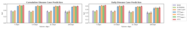
After the optimization on HT dataset, we load the CP factors of each method and conduct the tensor prediction task as described in the experimental setup. Specifically, we perform cumulative and daily disease case prediction, where for one particular ICD-10 code at one particular zipcode location, we predict how many more disease cases will happen within the future days.
The results are shown in Figure 6, where the dark bars are the standard deviations. The prediction results confirmed MTC and its variants outperform the baselines by up to about 20% on PoF.
6.6. Ablation Study on Initializations
To evaluate the multiresolution factorization part in MTC, we compare with other tensor initialization methods. Specifically, we implement the initialization from (i) other baselines: MRTL, TendiB; (ii) a typical tensor initialization method: HOSVD; (iii) no initialization, . For a fair comparison, we use the same optimization method (in Section 5) after different initializations.
Different amount of partial observations (i.e., different ) are considered: 5%, 2% and 1% on HT dataset. We report the first 30 iterations and the initialization time in Figure 7. Essentially, our MTC outperforms all other models after 30 iterations. One interesting finding is that TendiB and HOSVD start from the same PoF level regardless of the amount of partial observation since their initialization barely depends on the coarse views, i.e., and . However, with only a few iterations, MTC can surpass all baselines.

7. Conclusion
This paper identifies and solves a new problem: tensor completion from its partial and coarse observations. We formulate the problem into a generic couple-ALS form and propose an efficient completion model, MTC. The module combines multiresolution factorization and an effective optimization method as the treatment. We evaluate our MTC on two COVID-19 databases and show noticeable performance gain over the baseline methods.
Acknowledgements
This work was in part supported by the National Science Foundation award SCH-2014438, PPoSS 2028839, IIS-1838042, the National Institute of Health award NIH R01 1R01NS107291-01 and OSF Healthcare.
References
- (1)
- Acar et al. (2011a) Evrim Acar, Daniel M Dunlavy, Tamara G Kolda, and Morten Mørup. 2011a. Scalable tensor factorizations for incomplete data. Chemometrics and Intelligent Laboratory Systems (2011).
- Acar et al. (2011b) Evrim Acar, Tamara G Kolda, and Daniel M Dunlavy. 2011b. All-at-once optimization for coupled matrix and tensor factorizations. arXiv:1105.3422 (2011).
- Afshar et al. (2021) Ardavan Afshar, Kejing Yin, Sherry Yan, Cheng Qian, Joyce C Ho, Haesun Park, and Jimeng Sun. 2021. SWIFT: Scalable Wasserstein Factorization for Sparse Nonnegative Tensors. In AAAI.
- Ailon and Chazelle (2006) Nir Ailon and Bernard Chazelle. 2006. Approximate nearest neighbors and the fast Johnson-Lindenstrauss transform. In STOC. 557–563.
- Almutairi et al. (2020) Faisal M Almutairi, Charilaos I Kanatsoulis, and Nicholas D Sidiropoulos. 2020. Tendi: Tensor disaggregation from multiple coarse views. In PAKDD. Springer.
- Almutairi et al. (2021) Faisal M Almutairi, Charilaos I Kanatsoulis, and Nicholas D Sidiropoulos. 2021. PREMA: principled tensor data recovery from multiple aggregated views. IEEE Journal of Selected Topics in Signal Processing (2021).
- Araujo et al. (2017) Miguel Ramos Araujo, Pedro Manuel Pinto Ribeiro, and Christos Faloutsos. 2017. TensorCast: Forecasting with context using coupled tensors. In ICDM.
- Bahargam and Papalexakis (2018) Sanaz Bahargam and E. Papalexakis. 2018. Constrained coupled matrix-tensor factorization and its application in pattern and topic detection. In ASONAM.
- Barak and Moitra (2016) Boaz Barak and Ankur Moitra. 2016. Noisy tensor completion via the sum-of-squares hierarchy. In COLT. PMLR, 417–445.
- Borsoi et al. (2020) Ricardo Augusto Borsoi, Clémence Prévost, Konstantin Usevich, David Brie, José Carlos Moreira Bermudez, and C. Richard. 2020. Coupled Tensor Decomposition for Hyperspectral and Multispectral Image Fusion with Variability. arXiv (2020).
- Carroll and Chang (1970) J Douglas Carroll and Jih-Jie Chang. 1970. Analysis of individual differences in multidimensional scaling via an N-way generalization of “Eckart-Young” decomposition. Psychometrika 35, 3 (1970), 283–319.
- Eshragh et al. (2019) A. Eshragh, F. Roosta, A. Nazari, and M. Mahoney. 2019. LSAR: Efficient Leverage Score Sampling Algorithm for the Analysis of Big Time Series Data. arXiv (2019).
- Hitchcock (1927) Frank L Hitchcock. 1927. The expression of a tensor or a polyadic as a sum of products. Journal of Mathematics and Physics 6, 1-4 (1927), 164–189.
- Hong et al. (2020) David Hong, Tamara G Kolda, and Jed A Duersch. 2020. Generalized canonical polyadic tensor decomposition. SIAM Rev. 62, 1 (2020), 133–163.
- Huang et al. (2020) Huyan Huang, Yipeng Liu, and Ce Zhu. 2020. A Unified Framework for Coupled Tensor Completion. arXiv preprint arXiv:2001.02810 (2020).
- Kargas et al. (2021) Nikos Kargas, Cheng Qian, Nicholas D Sidiropoulos, Cao Xiao, Lucas M Glass, and Jimeng Sun. 2021. STELAR: Spatio-temporal Tensor Factorization with Latent Epidemiological Regularization. In AAAI.
- Karlsson et al. (2016) Lars Karlsson, Daniel Kressner, and André Uschmajew. 2016. Parallel Algorithms for Tensor Completion in the CP Format. Parallel Comput. 57, C (2016).
- Kolda and Bader (2009) Tamara G Kolda and Brett W Bader. 2009. Tensor decompositions and applications. SIAM review 51, 3 (2009), 455–500.
- Lacroix et al. (2018) Timothee Lacroix, Nicolas Usunier, and Guillaume Obozinski. 2018. Canonical Tensor Decomposition for Knowledge Base Completion. In ICML.
- Larsen and Kolda (2020) Brett W Larsen and Tamara G Kolda. 2020. Practical leverage-based sampling for low-rank tensor decomposition. arXiv preprint arXiv:2006.16438 (2020).
- Liu et al. (2012) Ji Liu, Przemyslaw Musialski, Peter Wonka, and Jieping Ye. 2012. Tensor completion for estimating missing values in visual data. IEEE TPAMI 35, 1 (2012).
- Özdemir et al. (2016) Alp Özdemir, Mark A Iwen, and Selin Aviyente. 2016. Multiscale tensor decomposition. In ACSSC. IEEE, 625–629.
- Park et al. (2020) J. Park, K. Carr, S. Zheng, Y. Yue, and R. Yu. 2020. Multiresolution Tensor Learning for Efficient and Interpretable Spatial Analysis. In ICML. PMLR, 7499–7509.
- Park and Ghosh (2014) Yubin Park and Joydeep Ghosh. 2014. Ludia: An aggregate-constrained low-rank reconstruction algorithm to leverage publicly released health data. In KDD.
- Schifanella et al. (2014) Claudio Schifanella, K Selçuk Candan, and Maria Luisa Sapino. 2014. Multiresolution tensor decompositions with mode hierarchies. TKDD 8, 2 (2014), 1–38.
- Sidiropoulos et al. (2017) Nicholas D Sidiropoulos, Lieven De Lathauwer, Xiao Fu, Kejun Huang, Evangelos E Papalexakis, and Christos Faloutsos. 2017. Tensor decomposition for signal processing and machine learning. IEEE TSP 65, 13 (2017), 3551–3582.
- Singh et al. (2021) Navjot Singh, Zecheng Zhang, Xiaoxiao Wu, Naijing Zhang, Siyuan Zhang, and Edgar Solomonik. 2021. Enabling distributed-memory tensor completion in Python using new sparse tensor kernels. arXiv preprint arXiv:1910.02371 (2021).
- Song et al. (2019) Qingquan Song, Hancheng Ge, James Caverlee, and Xia Hu. 2019. Tensor completion algorithms in big data analytics. ACM TKDD 13, 1 (2019), 1–48.
- Song et al. (2017) Qingquan Song, Xiao Huang, Hancheng Ge, James Caverlee, and Xia Hu. 2017. Multi-aspect streaming tensor completion. In KDD. 435–443.
- Sterck and Miller (2013) Hans De Sterck and Killian Miller. 2013. An adaptive algebraic multigrid algorithm for low-rank canonical tensor decomposition. SIAM SISC 35, 1 (2013), B1–B24.
- Wang et al. (2020) Senzhang Wang, Jiannong Cao, and Philip Yu. 2020. Deep learning for spatio-temporal data mining: A survey. TKDE (2020).
- Wang et al. (2015) Yichen Wang, Robert Chen, Joydeep Ghosh, Joshua C Denny, Abel Kho, You Chen, Bradley A Malin, and Jimeng Sun. 2015. Rubik: Knowledge guided tensor factorization and completion for health data analytics. In KDD.
- Xu and Yin (2013) Yangyang Xu and Wotao Yin. 2013. A block coordinate descent method for regularized multiconvex optimization with applications to nonnegative tensor factorization and completion. SIAM Journal on imaging sciences 6, 3 (2013).
- Yin et al. (2019) Kejing Yin, William K Cheung, Yang Liu, Benjamin CM Fung, and Jonathan Poon. 2019. Joint Learning of Phenotypes and Diagnosis-Medication Correspondence via Hidden Interaction Tensor Factorization.. In IJCAI.
Appendix A Basics of Tensor Computation
Kronecker Product.
One important product for matrices is Kroncker product. For and , their Kroncker product is defined by (each block is a scalar times matrix)
Khatri–Rao Product.
Khatri-Rao product is another important product for matrices, specifically, for matrices with same number of columns. The Khatri-Rao product of and can be viewed as column-wise Kroncker product,
where .
Tensor Unfolding.
This operation is to matricize a tensor along one mode. For tensor , we could unfold it along the first mode into a matrix (we use subscript notation). Specifically, each row of is a vectorization of a slab in the original tensor; we have
Similarly, for the unfolding operation along the second or third mode, we have
Hadamard Product.
The Hadamard product is the element-wise product for tensors of the same size. For example, the Hadamard product of two -mode tensors is
Appendix B Solver Implementation
We show the implementation of two stages in our solver.
Stage 1.
Suppose that we want to solve for the factor matrix , given Equation (5.2.2). To simplify the derivation, we assume
| (31) | ||||
| (32) |
The Jacobi method first decomposes into a diagonal matrix and an off-diagonal matrix , such that . After moving the off-diagonal part to the right, Equation (5.2.2) becomes
| (33) |
It is cheap to take the inverse of the diagonal (before the inverse, we add a small 1e-5 to the diagonal values to improve numerical stability) on both sides. The Jacobi iteration is given by the following recursive equation,
| (34) |
The convergence property is ensured by the largest absolute value of eigenvalues (i.e., spectral radius) of . If the the eigenvalues of are all in , then the iteration will converge. The iteration is enhanced by adding first-order momentum.
| (35) |
Now, the new spectral radius of is controlled by .
Stage 2.
This stage uses Cholesky decomposition to solve the joint normal equation. We use scipy.linalg.solve_triangular to get the exact solution.
Appendix C Details in Experiments
We list the GCSS data, processing files, the synthetic data, codes of our models, and all other baselines in an open repository.
C.1. Baseline Implementation
We provide more details about baselines used in the experiments:
-
•
CPC-ALS is a SOTA tensor completion method. It could be integrated with the sparse structure on parallel machines. The implementation could refer to (Karlsson et al., 2016). We provide our implementation in the link.
-
•
OracleCPD is implemented by standard CP decomposition on the original tensor, which provides the target low-rank factors. We implement it with our proposed solver. After convergence, the PoF results and objective functions are similar to the results provided by python Package tensorly.decomposition.parafac.
-
•
Block Gradient Descent (BGD) uses to replace in Equation (3.3), and then apply the block gradient descent algorithm. The learning rate is chosen by a binary line search algorithm with depth 3.
-
•
B-PREMA (Almutairi et al., 2021): this work is similar to BGD but with extra loss terms,
(36) ensuring that after the aggregation, the respective column sums of this two factors should be equal. Then, it also uses line search to find the learning rate.
-
•
CMTF-OPT (Acar et al., 2011b) is a popular model for coupled matrix and tensor factorization. We adopt it for coupled tensor factorization. Instead of alternatively optimizing factor matrices, it updates all factors at once. We use gradient descent to implement it, and the learning rate is also selected by line search.
-
•
MRTL (Park et al., 2020) designs a multiresolution tensor algorithm to build good initialization for accelerating their classification task. We adopt their tensor initialization method and compare it to our proposed multiresolution factorization.
-
•
TendiB (Almutairi et al., 2020) provides a heuristic initialization trick for the coupled factorization task. We only adopt its initialization based on our problem setting. In our case, we implement it as follows. We apply CPD on to estimate , and first, and then we freeze and use it to estimate and by applying another CPD on . We have also tried to interpolate and from the estimated and . However, it performs poorly. Consequently, we adopte the first implementation.
-
•
Higher-order singular value decomposition (HOSVD) (Kolda and Bader, 2009) is commonly used for initializing tensor CP-ALS decomposition. It first alternatively estimates orthogonal factors by higher-order orthogonal iteration (HOOI) and then applies ALS on the core tensor. The final initialization is the compositions of the orthogonal factor and core ALS factor. We adopt the HOSVD method as another initialization baseline.
C.2. Tasks and Metrics
We provide more details and rationality on the metrics.
-
•
Percentage of Fitness (PoF). Several performance evaluation metrics have been introduced in a survey paper (Song et al., 2019), and PoF is the most common one. For this metric, we also perform a two-tailed Student T-test and showe the -value in Table 3.
-
•
CPU Time. We make the methods execute for the same number of iterations and then compare their running time. The running time includes data loading, initialization (in our methods, it also includes the expense on low resolutions) and excludes the metric computation time.
-
•
Peak Memory. To evaluate space complexity, we record the memory usage during the optimization process and report the peak memory load.
C.3. Implementation and Hyperparameters
All the experiments are implemented by Python 3.7.8, scipy 1.5.2 and numpy 1.19.1 on Intel Cascade Lake Linux platform with 64 GB memory and 80 vCPU cores. By default, we conduct each experiment three times with different random seeds.
Since the CPD accepts an scaling invariance property, we apply the following trick after each iteration. For example, a set of factors would be identical to another factor set in terms of both the completion task or the prediction task. During the implementation of all models, we have adopted the following rescaling strategy to minimize the float-point round-off error:
| (37) | ||||
| (38) | ||||
| (39) |
where
| (40) |
which essentially equilibrates the norms of the factors of each component (we also do it for and ).
C.4. Experiments on Synthetic Data
The experiments on synthetic data verify our model in the ideal low-rank case.
Synthetic Tensor.
The data is generated by three uniformly randomed rank- factors with as the mode size consistently, . We sort each column of , to make sure the mode smoothness. Thus, a tensor is constructed, assuming that the first mode is categorical and the second/third modes are continuous. We also generate two aggregation matrix for the first and second modes, separately, to obtain coarse tensors, , .
Verification on Synthetic Data.
On the synthetic data, MTC is compared with three variants. We find that with only partially observed elements, all models can achieve near PoF, which is an exact completion of the low-rank synthetic . We thus further reduce the partial observation rate and consider three scenarios: (i) only observed data; (ii) observation with , where is unknown and is known; (iii) observation with , where are both unknown.

Results are shown in Figure 8. Basically, we conclude that: (i) our model is more advantageous with coarse level information; (ii) the multiresolution factorization and stage 1 are better used together.
C.5. Additional Experiments on GCSS with Known Aggregation
The main paper experiments do not use any aggregation information since, in those scenarios, the differences between model variants are clearer. This appendix supplies one aggregation matrix along the third model and shows that all our variants can achieve a similar tensor completion performance as OracleCPD.
Specifically, on GCSS dataset, we keep other settings unchanged and supply the aggregation matrix (from date to week) along the third mode. All variants converge quickly, and thus we only run the experiments for 50 iterations. The results are shown below.
| Model | PoF |
|---|---|
| OracleCPD | 0.7780 0.0012 |
| 0.7706 0.0058 | |
| 0.7694 0.0025 | |
| 0.7704 0.0037 | |
| MTC | 0.7708 0.0026 |