Yating [email protected]
\addauthorConghui [email protected]
\addauthorGim Hee [email protected]
\addinstitution
Department of Computer Science
National University of Singapore
Singapore
Audio-Visual Conditioned Video Prediction
Motion and Context-Aware Audio-Visual Conditioned Video Prediction
Abstract
The existing state-of-the-art method for audio-visual conditioned video prediction uses the latent codes of the audio-visual frames from a multimodal stochastic network and a frame encoder to predict the next visual frame. However, a direct inference of per-pixel intensity for the next visual frame is extremely challenging because of the high-dimensional image space. To this end, we decouple the audio-visual conditioned video prediction into motion and appearance modeling. The multimodal motion estimation predicts future optical flow based on the audio-motion correlation. The visual branch recalls from the motion memory built from the audio features to enable better long-term prediction. We further propose context-aware refinement to address the diminishing of the global appearance context in the long-term continuous warping. The global appearance context is extracted by the context encoder and manipulated by motion-conditioned affine transformation before fusion with features of warped frames. Experimental results show that our method achieves competitive results on existing benchmarks.

1 Introduction
Humans perceive the world via multisensory processing. Particularly, audio-visual interactions are ubiquitous in our daily life. For instance, a person at a bus stop perceives an approaching bus through both audio and visual cues, yet his/her view is suddenly blocked by another pedestrian. Despite this visual barrier, the person’s cognitive system can still fill in the missing visual content using previously seen frames and unbroken audio information. It has also been proven in neurobiology studies that such audio-visual pairing has the advantage of increasing the activation of neurons [Knöpfel et al.(2019)Knöpfel, Sweeney, Radulescu, Zabouri, Doostdar, Clopath, and Barnes] to enhance perceptual ability. Inspired by these observations, our aim is to investigate the feasibility of equipping machines with the capacity to leverage audio-visual interaction, employing audio-visual conditioned video prediction as a testbed.
Fig. 1 illustrates the audio-visual conditioned video prediction task. Given a full audio clip and a short sequence of the past visual frames, the objective is to predict the missing future visual frames that are as close to the ground truth frames as possible. The given audio clips and visual frames act as guidance in predicting the motion and appearance of future visual frames.
Existing state-of-the-art work Sound2Sight [Chatterjee and Cherian(2020)] proposes to directly infer per-pixel intensity, which contains both motion and appearance of future images, from the audio-visual inputs. A multi-modal stochastic network is used to encode the audio-visual information into a latent space distribution. A random vector drawn from this latent space distribution is then concatenated with the embedding of the current visual frame to simultaneously predict the motion and appearance of objects for the next visual frame, which is extremely challenging due to the high-dimensional nature of image space. As a result, Sound2Sight struggles to preserve the visual content in the generated visual frames, i.e. , the appearance of the digits in Fig. 4. We postulate that this inability to retain the visual content is caused by the tightly entangled motion and appearance modeling in Sound2Sight.
To this end, we model the motion and appearance separately in the audio-visual conditioned video prediction. We propose multimodal motion estimation (MME) to predict future object motion in the form of optical flow by using the audio-motion correlation. The rhythm of the sound and the object motion are naturally aligned since the sound originates from object motion [Blokhintzev(1946), Tijdeman(1975)]. Inspired by this natural phenomenon, we store the audio features in the motion memory to guide the visual motion prediction. In contrast to the internal memory in the ConvLSTMs that selectively remembers the past memory, the motion memory keeps all the past memory, which provides a good supplement in long-term motion prediction. To effectively bridge the audio-visual modality gap, we further design operator Condense to condense the large-size motion memory into a compact representation and operator Recall for the visual branch to use the audio motion context.
Although the next frame can now be generated by simply warping the current frame according to the predicted motion, the long-term continuous warping in the video prediction would result in the diminishing of the global appearance context. In order to effectively retain the appearance of objects, we creatively design a context-aware refinement (CAR) module. Other than just using a U-Net to refine the warped frames [Bei et al.(2021)Bei, Yang, and Soatto, Pan et al.(2019)Pan, Wang, Jia, Shao, Sheng, Yan, and Wang], we design a context encoder to supplement the global appearance context by extracting the visual features from the given past frame. Since the appearance details of each future frame may vary due to object movement, we perform the motion-conditioned affine transformation on the global context feature before inserting it into the U-Net decoder for better adaptation of the motion variance at each time step.
Our contributions in this paper are as follows:
-
•
We propose the multimodal motion estimation module to predict the optical flow of the next visual frame with the help of motion memory built from the audio features. We design the Condense and Recall operators to help the visual branch effectively utilize the audio motion memory.
-
•
We introduce the context-aware refinement module to mitigate the loss of global appearance context in the long-term warpings by using the context encoder and motion-conditioned affine transformation.
-
•
We conduct extensive experiments on both synthetic and real-world datasets to verify the effectiveness of our method.

2 Related Work
Video prediction. Video prediction estimates future video frames close to ground truth future frames conditioned on a few past frames. It can be divided into two categories: prediction in pixel space [Wang et al.(2017)Wang, Long, Wang, Gao, and Yu, Jin et al.(2020)Jin, Hu, Tang, Niu, Shi, Han, and Li, Xingjian et al.(2015)Xingjian, Chen, Wang, Yeung, Wong, and Woo, Lee et al.(2021a)Lee, Kim, Choi, Kim, and Ro, Wang et al.(2018b)Wang, Jiang, Yang, Li, Long, and Fei-Fei], and prediction in low-dimensional space [Lee et al.(2021b)Lee, Jung, Zhang, Chen, Koh, Huang, Yoon, Lee, and Hong, Villegas et al.(2017)Villegas, Yang, Zou, Sohn, Lin, and Lee, Villegas et al.(2018)Villegas, Erhan, Lee, et al., Wu et al.(2020)Wu, Gao, Park, and Chen]. Prediction in pixel space directly estimates the per-pixel intensity. For example, PredRNN [Wang et al.(2017)Wang, Long, Wang, Gao, and Yu] enables memory states to be updated across vertically stacked RNN layers and horizontally through all RNN states. Jin et al\bmvaOneDot[Jin et al.(2020)Jin, Hu, Tang, Niu, Shi, Han, and Li] adopt multi-level wavelet transform to deal with motion blur and missing appearance details. Denton and Fergus [Denton and Fergus(2018)] additionally consider stochasticity in the prediction by learning a prior distribution to capture the future dynamics.
Direct estimation of the per-pixel intensity of future visual frames is a very challenging task because of the high-dimensional image space. As a result, there are many works that seek to predict a low-dimensional representation, such as semantic map [Lee et al.(2021b)Lee, Jung, Zhang, Chen, Koh, Huang, Yoon, Lee, and Hong, Bei et al.(2021)Bei, Yang, and Soatto, Villar-Corrales et al.(2022)Villar-Corrales, Karapetyan, Boltres, and Behnke], human pose [Villegas et al.(2017)Villegas, Yang, Zou, Sohn, Lin, and Lee, Villar-Corrales et al.(2022)Villar-Corrales, Karapetyan, Boltres, and Behnke] and optical flow [Bei et al.(2021)Bei, Yang, and Soatto, Li et al.(2018)Li, Fang, Yang, Wang, Lu, and Yang, Liu et al.(2017)Liu, Yeh, Tang, Liu, and Agarwala, Liang et al.(2017)Liang, Lee, Dai, and Xing, Akan et al.(2021)Akan, Erdem, Erdem, and Güney]. Li et al\bmvaOneDot[Li et al.(2018)Li, Fang, Yang, Wang, Lu, and Yang] generate consecutive multiple future frames from only one image by multiple time step flow prediction and flow-to-frame synthesis. Bei et al\bmvaOneDot[Bei et al.(2021)Bei, Yang, and Soatto] first infer future optical flow and semantic maps independently for each object in the scene and then use U-Net to inpaint the future images. MSPred [Villar-Corrales et al.(2022)Villar-Corrales, Karapetyan, Boltres, and Behnke] simultaneously predicts future images and abstract representations via the hierarchical predictor module.
Different from the visual-only video prediction methods, we additionally consider the audio information. The pioneer work Sound2Sight [Chatterjee and Cherian(2020)] learns a joint audio-visual latent embedding to capture future dynamics. However, the latent codes cause the tight entanglement of motion and appearance, thus making it difficult for the model to balance the capture of correct motion and maintaining the shape of objects. Our solution is to model the motion and appearance separately through multimodal motion estimation and context-aware refinement, respectively.
Audio-visual representation learning. Audio-Visual representation learning learns a general representation in a self-supervised way by utilizing audio-visual correlation. There are mainly three types of correspondences: semantic similarity [Arandjelovic and Zisserman(2017), Aytar et al.(2016)Aytar, Vondrick, and Torralba, Arandjelovic and Zisserman(2018), Hu et al.(2019)Hu, Nie, and Li, Morgado et al.(2021)Morgado, Vasconcelos, and Misra], temporal consistency [Owens and Efros(2018), Korbar et al.(2018)Korbar, Tran, and Torresani, Afouras et al.(2020)Afouras, Owens, Chung, and Zisserman] and spatial correspondence [Gao et al.(2020)Gao, Chen, Al-Halah, Schissler, and Grauman, Yang et al.(2020)Yang, Russell, and Salamon]. Arandjelovic et al\bmvaOneDot[Arandjelovic and Zisserman(2017)] propose audio-visual correspondence learning by classifying whether the input audio and visual frame are from the same video or not. [Owens and Efros(2018)] design a pretext task to predict whether the audio stream and visual sequence are temporally aligned. [Yang et al.(2020)Yang, Russell, and Salamon] leverage audio-visual spatial correspondence by predicting whether the two channels of audio are flipped. In addition to learning a general representation, there are also many downstream audio-visual tasks, such as sound source localization [Chen et al.(2021)Chen, Xie, Afouras, Nagrani, Vedaldi, and Zisserman, Senocak et al.(2018)Senocak, Oh, Kim, Yang, and Kweon, Hu et al.(2020)Hu, Qian, Jiang, Tan, Wen, Ding, Lin, and Dou], audio-visual source separation [Gao and Grauman(2019), Zhao et al.(2018)Zhao, Gan, Rouditchenko, Vondrick, McDermott, and Torralba, Zhao et al.(2019)Zhao, Gan, Ma, and Torralba], audio-visual video parsing [Tian et al.(2020)Tian, Li, and Xu, Wu and Yang(2021)] and talking face generation [Chung et al.(2017)Chung, Jamaludin, and Zisserman, Chen et al.(2019)Chen, Maddox, Duan, and Xu, Vougioukas et al.(2018)Vougioukas, Petridis, and Pantic]. In this paper, we study the task of audio-visual conditioned video prediction and leverage audio-motion correlation.
3 Method
Problem definition. Let us denote a video with frames as , where represents a visual frame and its corresponding audio clip . A visual frame is an image of size , where is the number of channels, and are the width and height of the image. An audio clip is a two-dimensional spectrogram, where denotes the frequency range and represents the time duration of the audio clip. Given the first visual frames and the whole audio , the goal of the audio-visual conditioned video prediction task is to predict the missing visual frames to be as similar to the ground truth visual frames as possible. For brevity, we drop the frame index and denote the indices of the previous, current and next predicted frames as , and , respectively.
Method overview. Fig. 2 shows our proposed framework which consists of two modules: 1) multimodal motion estimation (MME) and 2) context-aware refinement (CAR). Our MME and CAR modules are designed to model motion and appearance, respectively. MME predicts future optical flow by taking visual and audio inputs. It stores the past and current audio information in the motion memory and the visual branch recalls from the condensed motion memory to better infer long-term future motions. CAR renders future frames by taking global appearance context into account. The warped images are supplemented with global appearance features extracted by the context encoder, and modulated by motion-conditioned affine transformation to get the final predicted future frames.
3.1 Multimodal Motion Estimation
The MME predicts optical flow in a recurrent way. For ease of warping, the MME operates on backward optical flow, i.e. both input and output are backward optical flow. We use both audio and visual modalities in this module because they both contain clear motion information. To predict the frame, the motion encoder takes the concatenation of the current optical flow and visual frame as inputs, and outputs the motion feature . Note that is a given visual frame if , otherwise it is generated by warping according to the predicted optical flow . We do not refine the warped image in MME. Concurrently, the audio encoder extracts the audio feature from input audio signal .
For our recurrent MME to effectively facilitate motion prediction, it is crucial to guarantee the presence of long-term memory for the audio information. However, the straightforward choice of LSTM is notorious for only having a short memory, where the memory cell is quickly saturated to remember only the latest input. As a result, it is difficult to infer long-term future motions. We thus design an external motion memory to store the audio features. In contrast to the memory cell inside LSTM that selectively remembers past memory, our motion memory keeps all the past memory without abandon. Our advantage is that it does not lose any past memory, and thus efficiently keeps all long-term information. The stores audio features up to time , . Then, visual features Recall from via cross-attention as the query , and is used to generate the key and value . During the long-term prediction, the size of increases linearly with the prediction length, making it difficult for the visual branch to catch useful information from the large motion memory. We address this motion memory complexity problem by Condensing the full into a compact memory as follows:
| (1) | ||||
where denotes the last slice of the memory. The operation follows [Wang et al.(2018a)Wang, Girshick, Gupta, and He]. The visual branch Recalls from the condensed audio memory and obtain the enhanced motion feature as follow:
| (2) |
We tile into the feature vector of size , where before computing Eqn. 2. is then fed into ConvLSTMs and motion decoder to predict optical flow at next time step as follows:
| (3) |
where is the hidden state and is the cell state of the ConvLSTMs at time step .

3.2 Context-Aware Refinement
The Context-Aware Refinement (CAR) module is then designed to generate the next visual frame according to the optical flow predicted by MME. Since audio cannot convey dense pixel information, we rely on the visual modality for appearance modeling. We start by warping the current visual frame using the predicted optical flow as follow:
| (4) |
where is the pixel coordinates. Similar to MME, is the given visual frame if , otherwise it is the output of CAR.
The warping procedure is performed recurrently by taking the current prediction as input and warping it into the next frame. It causes the warped image to become increasingly blurry and consequently leads to the loss of appearance context as shown in Fig. 3. The warped images gradually lose the shape of the brush.
To alleviate the blurry visual frame problem, we first use a U-Net [Ronneberger et al.(2015)Ronneberger, Fischer, and Brox] to refine the local details. Furthermore, we address the loss of appearance context by providing external appearance information. The context encoder extracts global appearance context from the last given visual frame . is the feature at the -th layer of and is the total number of layers. The context encoder resembles the U-Net encoder in its design, albeit shallower structure. Given the varying appearance of each frame caused by object motion, it is necessary to adjust the global context accordingly for effective prediction. Inspired by the success of text-image fusion using affine transformation [Tao et al.(2020)Tao, Tang, Wu, Sebe, Jing, Wu, and Bao], we propose motion-conditioned affine transformation to refine the global context for each frame. We first obtain the motion feature by concatenating the output of the motion encoder and audio encoder as follow:
| (5) |
where denotes the concatenation operation. We also employ audio to compute as it contains motion-related information. The transformation parameters and for the global context feature at the -th layer are obtained from two separate MLPs, which are both conditioned on motion feature so that the transformed feature is able to adapt to motion variance:
| (6) |
Then, channel-wise scaling and shifting is performed on to obtain the adapted context :
| (7) |
Finally, we insert into its corresponding layer in the U-Net decoder.
3.3 Optimization
We train our model in two stages due to the different convergence speeds of MME and CAR. We optimize MME in the first stage, and then we fix MME and optimize CAR in the second stage. We train MME by optimizing an optical flow reconstruction loss and a smoothness regularization term :
| (8) |
where is a weighting hyperparameter for . computes a mean-squared error between the predicted optical flow and ground truth optical flow as follows:
| (9) |
Following [Wu et al.(2020)Wu, Gao, Park, and Chen, Yin and Shi(2018)], we have a smoothness regularization term for our optical flow estimation:
| (10) |
where is the gradient operator. The supervision for CAR is an image reconstruction loss , which computes the mean-squared error between the predicted and ground truth frames:
| (11) |
4 Experiments
| Method | Type | SSIM | PSNR | ||||||
|---|---|---|---|---|---|---|---|---|---|
| Fr 6 | Fr 15 | Fr 25 | Mean | Fr 6 | Fr 15 | Fr 25 | Mean | ||
| Denton and Fergus [Denton and Fergus(2018)] | V | ||||||||
| MSPred [Villar-Corrales et al.(2022)Villar-Corrales, Karapetyan, Boltres, and Behnke] | V | 0.9400 | 0.8903 | 0.8060 | 0.8846 | 21.57 | 19.02 | 17.04 | 19.08 |
| Vougioukas et al\bmvaOneDot[Vougioukas et al.(2018)Vougioukas, Petridis, and Pantic] | M | ||||||||
| Sound2Sight [Chatterjee and Cherian(2020)] | M | ||||||||
| Our Method | M | 0.9608 | 0.9158 | 0.8990 | 0.9195 | 23.61 | 19.88 | 18.99 | 20.23 |
Datasets. We conduct experiments on both synthetic and real-world datasets taken from [Chatterjee and Cherian(2020)]: 1) Multimodal MovingMNIST. This dataset is an extension of stochastic MovingMNIST [Srivastava et al.(2015)Srivastava, Mansimov, and Salakhudinov] by adding artificial sound. Although MovingMNIST is synthetic, it is a standard benchmark in video prediction [Wang et al.(2018b)Wang, Jiang, Yang, Li, Long, and Fei-Fei, Lee et al.(2021a)Lee, Kim, Choi, Kim, and Ro, Denton and Fergus(2018)]. In Multimodal MovingMNIST, each digit is equipped with a unique tone and the amplitude of the tone is inversely proportional to the distance of the digit from the origin. The sound changes momentarily whenever the digit hits the boundary. This dataset consists of 8,000 training and 1,000 test videos. 2) YouTube Painting. It contains painting videos from YouTube. In each video, a painter is painting on a canvas in an indoor environment and there is a clear sound of the brush strokes. It contains training, and 500 test videos. Each video is of 64 64 resolution, 30fps, and 3 seconds long. 3) AudioSet-Drums. This dataset contains selected videos from the drums class of AudioSet [Gemmeke et al.(2017)Gemmeke, Ellis, Freedman, Jansen, Lawrence, Moore, Plakal, and Ritter]. The video clips are selected such that the drum player is visible when the drum beat is audible. It contains training, and test videos. Each video is of 64 × 64 resolution, 30fps, and 3 seconds long.
Implementation. The video frames are resized to in Multimodal MovingMNIST and in YouTube Painting and AudioSet-Drums. The intensity values of the video frames are normalized into . We directly use the precomputed spectrogram by [Chatterjee and Cherian(2020)] as audio input. We use the Adam optimizer [Kingma and Ba(2014)] and the learning rate is set to and for MME and CAR, respectively. The coefficient is set to 0.01. We use 4-layer ConvLSTMs in MME and insert layers of context feature in CAR. Ground truth optical flow is precomputed using the TV-L1 algorithm from [Zach et al.(2007)Zach, Pock, and Bischof]. We implement our framework with Pytorch on two Nvidia GeForce GTX1080Ti GPUs.
Evaluation setup. On Multimodal MovingMNIST, we show 5 initial frames and full audio, and we predict the next 15 frames during training and 20 frames during evaluation. On YouTube Painting and AudioSet-Drums, we show 15 initial visual frames and full audio, and predict the next 15 visual frames during training and 30 visual frames during evaluation. We evaluate our method by the structure similarity (SSIM) [Wang et al.(2004)Wang, Bovik, Sheikh, and Simoncelli] and Peak Signal to Noise Ratio (PSNR). We report SSIM and PSNR on selected visual frames. The mean SSIM and PSNR of the full predicted sequence are also reported to represent average performance.
4.1 Results

We compare our results with Sound2Sight [Chatterjee and Cherian(2020)], Vougioukas et al\bmvaOneDot[Vougioukas et al.(2018)Vougioukas, Petridis, and Pantic], MSPred [Villar-Corrales et al.(2022)Villar-Corrales, Karapetyan, Boltres, and Behnke] and Denton and Fergu [Denton and Fergus(2018)]. We re-run the source code of Sound2Sight [Chatterjee and Cherian(2020)] to compute the average score over 100 times of sampling instead of using the best result of the samples drawn from sampling reported by Sound2sight. In practice, it is statistically more meaningful to use the mean instead of the best result since the stochastic approach cannot always achieve the highest result in every sampling. Moreover, we do not know the ground truths of future visual frames. Therefore, it is unreasonable for [Chatterjee and Cherian(2020)] to search for the best samples drawn from their stochastic model using the ground truths.
| Method | Type | SSIM | PSNR | ||||||
|---|---|---|---|---|---|---|---|---|---|
| Fr 16 | Fr 30 | Fr 45 | Mean | Fr 16 | Fr 30 | Fr 45 | Mean | ||
| Denton and Fergus [Denton and Fergus(2018)] | V | ||||||||
| MSPred [Villar-Corrales et al.(2022)Villar-Corrales, Karapetyan, Boltres, and Behnke] | V | 0.9648 | 0.8991 | 0.8617 | 0.8965 | 33.42 | 26.42 | 24.25 | 26.65 |
| Vougioukas et al\bmvaOneDot[Vougioukas et al.(2018)Vougioukas, Petridis, and Pantic] | M | ||||||||
| Sound2Sight [Chatterjee and Cherian(2020)] | M | ||||||||
| Our Method | M | 0.9848 | 0.9284 | 0.9104 | 0.9313 | 35.12 | 27.19 | 25.53 | 27.70 |
| Method | Type | SSIM | PSNR | ||||||
|---|---|---|---|---|---|---|---|---|---|
| Fr 16 | Fr 30 | Fr 45 | Mean | Fr 16 | Fr 30 | Fr 45 | Mean | ||
| Denton and Fergus [Denton and Fergus(2018)] | V | ||||||||
| MSPred [Villar-Corrales et al.(2022)Villar-Corrales, Karapetyan, Boltres, and Behnke] | V | 0.9799 | 0.9382 | 0.9214 | 0.9389 | 33.55 | 27.30 | 25.91 | 27.60 |
| Vougioukas et al\bmvaOneDot[Vougioukas et al.(2018)Vougioukas, Petridis, and Pantic] | M | ||||||||
| Sound2Sight [Chatterjee and Cherian(2020)] | M | 26.71 | |||||||
| Our Method | M | 0.9896 | 0.9533 | 0.9437 | 0.9558 | 35.00 | 27.76 | 28.22 | |
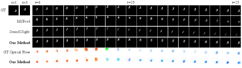
Multimodal MovingMNIST. Tab. 1 shows quantitative results on Multimodal MovingMNIST. Our method outperforms others by a large margin across all time steps. Fig. 4 shows the quantitative results. The first four rows show the comparison of the predicted visual frames sequence. The last two rows show the corresponding optical flow results. We follow the flow color coding of [Baker et al.(2011)Baker, Scharstein, Lewis, Roth, Black, and Szeliski]. It can be seen that our method is able to correctly predict the trajectory and also maintain the complex shape of digit ‘3’ in long-term prediction. On the contrary, the predicted sequence from Sound2Sight and MSPred gradually lose the shape of the digit or even deviate from the correct trajectory.
YouTube Painting. Tab. 2 shows quantitative results on YouTube Painting. Our model again surpasses other methods. Fig. 5 shows the qualitative comparison with Sound2Sight. Due to entangled modeling of motion and appearance, the result of Sound2Sight gradually loses the shape of the hand. Furthermore, the hand becomes stationary at the top right corner of the image. In contrast, our model maintains a relatively good appearance and generally follows the movement of the hand in ground truth frames. We can also see that our predicted optical flows are close to the ground truths.
AudioSet-Drums. Tab. 3 shows quantitative results on AudioSet-Drums. Our model surpasses others at almost every time step. We notice that our superiority is not as obvious on AudioSet-Drums as on the other two datasets. The reason may be that motion only exists in a small region of frames in AudioSet-Drums, and is hard for our model to fully capture it. Nevertheless, our model still achieves the best overall result.
| Method | YouTube | MNIST | AudioSet |
|---|---|---|---|
| V | |||
| V + Recall | |||
| MME | 9.85 | 4.82 | 3.97 |
| Method | SSIM | |||
|---|---|---|---|---|
| Fr 16 | Fr 30 | Fr 45 | Mean | |
| MME+Unet | 0.9873 | |||
| MME+Unet+ContextEnc | ||||
| MME+CAR | 0.9284 | 0.9104 | 0.9313 | |
4.2 Ablation Study
Effectiveness of audio-motion correlation in MME. As audio is directly influencing optical flow prediction, we analyze the effectiveness of audio in MME. We compare the quality of optical flow using average endpoint error (AEPE) [Sun et al.(2018)Sun, Yang, Liu, and Kautz, Ilg et al.(2017)Ilg, Mayer, Saikia, Keuper, Dosovitskiy, and Brox] in Tab. 5. The baseline ‘V’ predicts optical flow without audio. ‘V+Recall’ Recall from audio motion memory, but does not condense it. ‘MME’ is our full model in stage 1 with both condense and recall. MME has the lowest error in the flow prediction, suggesting the audio is effective in helping the visual motion prediction.
Effectiveness of Context-Aware Refinement. We analyze context-aware refinement (CAR) in Tab. 5. ‘MME+Unet’ only uses U-Net for refinement in stage 2. ‘MME+Unet+ContextEnc’ adds a context encoder but does not perform affine transformation over the context feature. ‘MME+CAR’ is our full model with motion-conditioned affine transformation. We can see from the first and second rows that a single U-Net is insufficient to model image appearance in long-term prediction, and thus it is very important to supply additional context information. We can see from the second and last rows that our motion-conditioned affine transformation is able to adjust the global context feature for better performance in long-term predictions.
| Method | Fr 16 | Fr 30 | Fr 45 | Mean |
|---|---|---|---|---|
| Sound2Sight [Chatterjee and Cherian(2020)] | 0.9556 | 0.9107 | 0.8936 | 0.9117 |
| Ours | 0.9827 | 0.9252 | 0.9069 | 0.9280 |
Input video with higher resolution. We use the video frames of original resolution as input. The results are shown in Tab. 6. Our model consistently outperforms [Chatterjee and Cherian(2020)], demonstrating its effectiveness even when provided with higher-resolution videos.
5 Conclusions
In this paper, we address the task of audio-visual conditioned video prediction by decoupling it into motion and appearance. We design the MME and CAR by considering the influence of audio and visual modalities in each component. MME leverages audio-motion correlation by using audio as an external motion memory in predicting future optical flow. CAR addresses the loss of appearance context in long-term prediction by adding a context encoder. To make the global context feature compatible with motion variance, we perform the motion-conditioned affine transformation to adjust the feature. The effectiveness of our proposed method is analyzed both quantitatively and qualitatively.
Acknowledgement.
This research is supported by the National Research Foundation, Singapore under its AI Singapore Programme (AISG Award No: AISG2-RP-2021-024), and the Tier 2 grant MOE-T2EP20120-0011 from the Singapore Ministry of Education.
Supplementary Material
Appendix A Qualitative Ablation Study
We conduct qualitative analysis to verify the effectiveness of MME and CAR.
Effectiveness of audio-motion correlation in MME. Fig. A1 presents the qualitative comparion of different motion estimation networks. ‘GT Flow’ is the ground truth optical flow. The baseline ‘V’ predicts optical flow without audio. ‘V+Recall’ Recall from audio motion memory, but does not condense it. ‘MME’ is our full model in stage 1 with both condense and recall. It is clear to see that only using visual modality (‘V’) to predict motion has the worst prediction. Although ‘V+Recall’ captures the correct motion in the short term, it fails at longer future due to its large-size motion memory. In contrast, MME has a better balance in both short-term and long-term predictions due to the condensed memory.

Effectiveness of Context-Aware Refinement. Fig. A2 presents the qualitative comparison of different image refinement networks. ‘Unet’ only uses U-Net for refinement in stage 2. ‘Unet+ContextEnc’ adds a context encoder but does not perform affine transformation over the context feature. It shows that CAR is able to provide and aggregate the feature of hand and pen to make the moving object more concrete.

Appendix B Qualitative Video Results
We provide a video (‘video results.mp4’) to show the prediction by our model and the ground truth in the supplementary zip file. The white denotes ground truth and the red denotes prediction. Video 1 and video 2 show 15 past frames and 30 future frames. Video 3 and 4 show 5 past frames and 20 future frames. Our prediction is temporally smooth and consistent with the ground truth audio and visual frames.
Appendix C Architecture Details
We present the detailed architecture of our proposed framework.
Motion Encoder. The motion encoder consists of four convolutional layers with kernel size of and stride of 2. The number of channels is . Each convolutional layer is followed by Batch Normalization and Leaky ReLU, except for the last layer which is followed by Batch Normalization and Tanh.
Motion Decoder. The motion decoder consists of four deconvolution layers with kernel size of and stride of 2. The number of channels is . Each convolutional layer is followed by Batch Normalization and Leaky ReLU, except for the last layer.
Audio Encoder. The audio encoder consists of five convolutional layers with kernel size of for the first four layers and with kernel size of for the last layer. The number of channels is . Each convolutional layer is followed by Batch Normalization and Leaky ReLU, except for the last layer which is followed by Batch Normalization and Tanh.
Condense and Recall. The operators and use attention mechanism as shown in Fig C3. Specifically, Operator takes the motion memory as input and projects it into the query , key and value via three separate 1D convolutional layers with kernel size of 1, respectively. In , the visual feature is sent into a 2D convolutional layer with kernel size of and then is flattened along spatial dimensions as . The condensed memory is sent into two separate 1D convolutional layers with kernel size of 1 and projected as and , respectively.
Context Encoder. The context encoder has four blocks, where each block consists of two convolutional layers followed by Batch Normalization and ReLU. A max pooling layer is inserted between adjacent blocks.

References
- [Afouras et al.(2020)Afouras, Owens, Chung, and Zisserman] Triantafyllos Afouras, Andrew Owens, Joon Son Chung, and Andrew Zisserman. Self-supervised learning of audio-visual objects from video. In Computer Vision–ECCV 2020: 16th European Conference, Glasgow, UK, August 23–28, 2020, Proceedings, Part XVIII 16, pages 208–224. Springer, 2020.
- [Akan et al.(2021)Akan, Erdem, Erdem, and Güney] Adil Kaan Akan, Erkut Erdem, Aykut Erdem, and Fatma Güney. Slamp: Stochastic latent appearance and motion prediction. In Proceedings of the IEEE/CVF International Conference on Computer Vision, pages 14728–14737, 2021.
- [Arandjelovic and Zisserman(2017)] Relja Arandjelovic and Andrew Zisserman. Look, listen and learn. In Proceedings of the IEEE International Conference on Computer Vision, pages 609–617, 2017.
- [Arandjelovic and Zisserman(2018)] Relja Arandjelovic and Andrew Zisserman. Objects that sound. In Proceedings of the European conference on computer vision (ECCV), pages 435–451, 2018.
- [Aytar et al.(2016)Aytar, Vondrick, and Torralba] Yusuf Aytar, Carl Vondrick, and Antonio Torralba. Soundnet: Learning sound representations from unlabeled video. Advances in neural information processing systems, 29:892–900, 2016.
- [Baker et al.(2011)Baker, Scharstein, Lewis, Roth, Black, and Szeliski] Simon Baker, Daniel Scharstein, JP Lewis, Stefan Roth, Michael J Black, and Richard Szeliski. A database and evaluation methodology for optical flow. International journal of computer vision, 92(1):1–31, 2011.
- [Bei et al.(2021)Bei, Yang, and Soatto] Xinzhu Bei, Yanchao Yang, and Stefano Soatto. Learning semantic-aware dynamics for video prediction. In Proceedings of the IEEE/CVF Conference on Computer Vision and Pattern Recognition, pages 902–912, 2021.
- [Blokhintzev(1946)] D Blokhintzev. The propagation of sound in an inhomogeneous and moving medium i. The Journal of the Acoustical Society of America, 18(2):322–328, 1946.
- [Chatterjee and Cherian(2020)] Moitreya Chatterjee and Anoop Cherian. Sound2sight: Generating visual dynamics from sound and context. In European Conference on Computer Vision, pages 701–719. Springer, 2020.
- [Chen et al.(2021)Chen, Xie, Afouras, Nagrani, Vedaldi, and Zisserman] Honglie Chen, Weidi Xie, Triantafyllos Afouras, Arsha Nagrani, Andrea Vedaldi, and Andrew Zisserman. Localizing visual sounds the hard way. In Proceedings of the IEEE/CVF Conference on Computer Vision and Pattern Recognition, pages 16867–16876, 2021.
- [Chen et al.(2019)Chen, Maddox, Duan, and Xu] Lele Chen, Ross K Maddox, Zhiyao Duan, and Chenliang Xu. Hierarchical cross-modal talking face generation with dynamic pixel-wise loss. In Proceedings of the IEEE/CVF Conference on Computer Vision and Pattern Recognition, pages 7832–7841, 2019.
- [Chung et al.(2017)Chung, Jamaludin, and Zisserman] Joon Son Chung, Amir Jamaludin, and Andrew Zisserman. You said that? arXiv preprint arXiv:1705.02966, 2017.
- [Denton and Fergus(2018)] Emily Denton and Rob Fergus. Stochastic video generation with a learned prior. In International Conference on Machine Learning, pages 1174–1183. PMLR, 2018.
- [Gao and Grauman(2019)] Ruohan Gao and Kristen Grauman. Co-separating sounds of visual objects. In Proceedings of the IEEE/CVF International Conference on Computer Vision, pages 3879–3888, 2019.
- [Gao et al.(2020)Gao, Chen, Al-Halah, Schissler, and Grauman] Ruohan Gao, Changan Chen, Ziad Al-Halah, Carl Schissler, and Kristen Grauman. Visualechoes: Spatial image representation learning through echolocation. In European Conference on Computer Vision, pages 658–676. Springer, 2020.
- [Gemmeke et al.(2017)Gemmeke, Ellis, Freedman, Jansen, Lawrence, Moore, Plakal, and Ritter] Jort F Gemmeke, Daniel PW Ellis, Dylan Freedman, Aren Jansen, Wade Lawrence, R Channing Moore, Manoj Plakal, and Marvin Ritter. Audio set: An ontology and human-labeled dataset for audio events. In 2017 IEEE International Conference on Acoustics, Speech and Signal Processing (ICASSP), pages 776–780. IEEE, 2017.
- [Hu et al.(2019)Hu, Nie, and Li] Di Hu, Feiping Nie, and Xuelong Li. Deep multimodal clustering for unsupervised audiovisual learning. In Proceedings of the IEEE/CVF Conference on Computer Vision and Pattern Recognition, pages 9248–9257, 2019.
- [Hu et al.(2020)Hu, Qian, Jiang, Tan, Wen, Ding, Lin, and Dou] Di Hu, Rui Qian, Minyue Jiang, Xiao Tan, Shilei Wen, Errui Ding, Weiyao Lin, and Dejing Dou. Discriminative sounding objects localization via self-supervised audiovisual matching. Advances in Neural Information Processing Systems, 33, 2020.
- [Ilg et al.(2017)Ilg, Mayer, Saikia, Keuper, Dosovitskiy, and Brox] Eddy Ilg, Nikolaus Mayer, Tonmoy Saikia, Margret Keuper, Alexey Dosovitskiy, and Thomas Brox. Flownet 2.0: Evolution of optical flow estimation with deep networks. In Proceedings of the IEEE conference on computer vision and pattern recognition, pages 2462–2470, 2017.
- [Jin et al.(2020)Jin, Hu, Tang, Niu, Shi, Han, and Li] Beibei Jin, Yu Hu, Qiankun Tang, Jingyu Niu, Zhiping Shi, Yinhe Han, and Xiaowei Li. Exploring spatial-temporal multi-frequency analysis for high-fidelity and temporal-consistency video prediction. In Proceedings of the IEEE/CVF Conference on Computer Vision and Pattern Recognition, pages 4554–4563, 2020.
- [Kingma and Ba(2014)] Diederik P Kingma and Jimmy Ba. Adam: A method for stochastic optimization. arXiv preprint arXiv:1412.6980, 2014.
- [Knöpfel et al.(2019)Knöpfel, Sweeney, Radulescu, Zabouri, Doostdar, Clopath, and Barnes] Thomas Knöpfel, Yann Sweeney, Carola I Radulescu, Nawal Zabouri, Nazanin Doostdar, Claudia Clopath, and Samuel J Barnes. Audio-visual experience strengthens multisensory assemblies in adult mouse visual cortex. Nature communications, 10(1):1–15, 2019.
- [Korbar et al.(2018)Korbar, Tran, and Torresani] Bruno Korbar, Du Tran, and Lorenzo Torresani. Cooperative learning of audio and video models from self-supervised synchronization. arXiv preprint arXiv:1807.00230, 2018.
- [Lee et al.(2021a)Lee, Kim, Choi, Kim, and Ro] Sangmin Lee, Hak Gu Kim, Dae Hwi Choi, Hyung-Il Kim, and Yong Man Ro. Video prediction recalling long-term motion context via memory alignment learning. In Proceedings of the IEEE/CVF Conference on Computer Vision and Pattern Recognition, pages 3054–3063, 2021a.
- [Lee et al.(2021b)Lee, Jung, Zhang, Chen, Koh, Huang, Yoon, Lee, and Hong] Wonkwang Lee, Whie Jung, Han Zhang, Ting Chen, Jing Yu Koh, Thomas Huang, Hyungsuk Yoon, Honglak Lee, and Seunghoon Hong. Revisiting hierarchical approach for persistent long-term video prediction. arXiv preprint arXiv:2104.06697, 2021b.
- [Li et al.(2018)Li, Fang, Yang, Wang, Lu, and Yang] Yijun Li, Chen Fang, Jimei Yang, Zhaowen Wang, Xin Lu, and Ming-Hsuan Yang. Flow-grounded spatial-temporal video prediction from still images. In Proceedings of the European Conference on Computer Vision (ECCV), pages 600–615, 2018.
- [Liang et al.(2017)Liang, Lee, Dai, and Xing] Xiaodan Liang, Lisa Lee, Wei Dai, and Eric P Xing. Dual motion gan for future-flow embedded video prediction. In proceedings of the IEEE international conference on computer vision, pages 1744–1752, 2017.
- [Liu et al.(2017)Liu, Yeh, Tang, Liu, and Agarwala] Ziwei Liu, Raymond A Yeh, Xiaoou Tang, Yiming Liu, and Aseem Agarwala. Video frame synthesis using deep voxel flow. In Proceedings of the IEEE international conference on computer vision, pages 4463–4471, 2017.
- [Morgado et al.(2021)Morgado, Vasconcelos, and Misra] Pedro Morgado, Nuno Vasconcelos, and Ishan Misra. Audio-visual instance discrimination with cross-modal agreement. In Proceedings of the IEEE/CVF Conference on Computer Vision and Pattern Recognition, pages 12475–12486, 2021.
- [Owens and Efros(2018)] Andrew Owens and Alexei A Efros. Audio-visual scene analysis with self-supervised multisensory features. In Proceedings of the European Conference on Computer Vision (ECCV), pages 631–648, 2018.
- [Pan et al.(2019)Pan, Wang, Jia, Shao, Sheng, Yan, and Wang] Junting Pan, Chengyu Wang, Xu Jia, Jing Shao, Lu Sheng, Junjie Yan, and Xiaogang Wang. Video generation from single semantic label map. In Proceedings of the IEEE/CVF Conference on Computer Vision and Pattern Recognition, pages 3733–3742, 2019.
- [Ronneberger et al.(2015)Ronneberger, Fischer, and Brox] Olaf Ronneberger, Philipp Fischer, and Thomas Brox. U-net: Convolutional networks for biomedical image segmentation. In International Conference on Medical image computing and computer-assisted intervention, pages 234–241. Springer, 2015.
- [Senocak et al.(2018)Senocak, Oh, Kim, Yang, and Kweon] Arda Senocak, Tae-Hyun Oh, Junsik Kim, Ming-Hsuan Yang, and In So Kweon. Learning to localize sound source in visual scenes. In Proceedings of the IEEE Conference on Computer Vision and Pattern Recognition, pages 4358–4366, 2018.
- [Srivastava et al.(2015)Srivastava, Mansimov, and Salakhudinov] Nitish Srivastava, Elman Mansimov, and Ruslan Salakhudinov. Unsupervised learning of video representations using lstms. In International conference on machine learning, pages 843–852. PMLR, 2015.
- [Sun et al.(2018)Sun, Yang, Liu, and Kautz] Deqing Sun, Xiaodong Yang, Ming-Yu Liu, and Jan Kautz. Pwc-net: Cnns for optical flow using pyramid, warping, and cost volume. In Proceedings of the IEEE conference on computer vision and pattern recognition, pages 8934–8943, 2018.
- [Tao et al.(2020)Tao, Tang, Wu, Sebe, Jing, Wu, and Bao] Ming Tao, Hao Tang, Songsong Wu, Nicu Sebe, Xiao-Yuan Jing, Fei Wu, and Bingkun Bao. Df-gan: Deep fusion generative adversarial networks for text-to-image synthesis. arXiv preprint arXiv:2008.05865, 2020.
- [Tian et al.(2020)Tian, Li, and Xu] Yapeng Tian, Dingzeyu Li, and Chenliang Xu. Unified multisensory perception: Weakly-supervised audio-visual video parsing. In Computer Vision–ECCV 2020: 16th European Conference, Glasgow, UK, August 23–28, 2020, Proceedings, Part III 16, pages 436–454. Springer, 2020.
- [Tijdeman(1975)] H Tijdeman. On the propagation of sound waves in cylindrical tubes. Journal of Sound and Vibration, 39(1):1–33, 1975.
- [Villar-Corrales et al.(2022)Villar-Corrales, Karapetyan, Boltres, and Behnke] Angel Villar-Corrales, Ani Karapetyan, Andreas Boltres, and Sven Behnke. Mspred: Video prediction at multiple spatio-temporal scales with hierarchical recurrent networks. In British Machine Vision Conference (BMVC), 2022.
- [Villegas et al.(2017)Villegas, Yang, Zou, Sohn, Lin, and Lee] Ruben Villegas, Jimei Yang, Yuliang Zou, Sungryull Sohn, Xunyu Lin, and Honglak Lee. Learning to generate long-term future via hierarchical prediction. In international conference on machine learning, pages 3560–3569. PMLR, 2017.
- [Villegas et al.(2018)Villegas, Erhan, Lee, et al.] Ruben Villegas, Dumitru Erhan, Honglak Lee, et al. Hierarchical long-term video prediction without supervision. In International Conference on Machine Learning, pages 6038–6046. PMLR, 2018.
- [Vougioukas et al.(2018)Vougioukas, Petridis, and Pantic] Konstantinos Vougioukas, Stavros Petridis, and Maja Pantic. End-to-end speech-driven facial animation with temporal gans. arXiv preprint arXiv:1805.09313, 2018.
- [Wang et al.(2018a)Wang, Girshick, Gupta, and He] Xiaolong Wang, Ross Girshick, Abhinav Gupta, and Kaiming He. Non-local neural networks. In Proceedings of the IEEE conference on computer vision and pattern recognition, pages 7794–7803, 2018a.
- [Wang et al.(2017)Wang, Long, Wang, Gao, and Yu] Yunbo Wang, Mingsheng Long, Jianmin Wang, Zhifeng Gao, and Philip S Yu. Predrnn: Recurrent neural networks for predictive learning using spatiotemporal lstms. In Proceedings of the 31st International Conference on Neural Information Processing Systems, pages 879–888, 2017.
- [Wang et al.(2018b)Wang, Jiang, Yang, Li, Long, and Fei-Fei] Yunbo Wang, Lu Jiang, Ming-Hsuan Yang, Li-Jia Li, Mingsheng Long, and Li Fei-Fei. Eidetic 3d lstm: A model for video prediction and beyond. In International conference on learning representations, 2018b.
- [Wang et al.(2004)Wang, Bovik, Sheikh, and Simoncelli] Zhou Wang, Alan C Bovik, Hamid R Sheikh, and Eero P Simoncelli. Image quality assessment: from error visibility to structural similarity. IEEE transactions on image processing, 13(4):600–612, 2004.
- [Wu and Yang(2021)] Yu Wu and Yi Yang. Exploring heterogeneous clues for weakly-supervised audio-visual video parsing. In Proceedings of the IEEE/CVF Conference on Computer Vision and Pattern Recognition, pages 1326–1335, 2021.
- [Wu et al.(2020)Wu, Gao, Park, and Chen] Yue Wu, Rongrong Gao, Jaesik Park, and Qifeng Chen. Future video synthesis with object motion prediction. In Proceedings of the IEEE/CVF Conference on Computer Vision and Pattern Recognition, pages 5539–5548, 2020.
- [Xingjian et al.(2015)Xingjian, Chen, Wang, Yeung, Wong, and Woo] SHI Xingjian, Zhourong Chen, Hao Wang, Dit-Yan Yeung, Wai-Kin Wong, and Wang-chun Woo. Convolutional lstm network: A machine learning approach for precipitation nowcasting. In Advances in neural information processing systems, pages 802–810, 2015.
- [Yang et al.(2020)Yang, Russell, and Salamon] Karren Yang, Bryan Russell, and Justin Salamon. Telling left from right: Learning spatial correspondence of sight and sound. In Proceedings of the IEEE/CVF Conference on Computer Vision and Pattern Recognition, pages 9932–9941, 2020.
- [Yin and Shi(2018)] Zhichao Yin and Jianping Shi. Geonet: Unsupervised learning of dense depth, optical flow and camera pose. In Proceedings of the IEEE conference on computer vision and pattern recognition, pages 1983–1992, 2018.
- [Zach et al.(2007)Zach, Pock, and Bischof] Christopher Zach, Thomas Pock, and Horst Bischof. A duality based approach for realtime tv-l 1 optical flow. In Joint pattern recognition symposium, pages 214–223. Springer, 2007.
- [Zhao et al.(2018)Zhao, Gan, Rouditchenko, Vondrick, McDermott, and Torralba] Hang Zhao, Chuang Gan, Andrew Rouditchenko, Carl Vondrick, Josh McDermott, and Antonio Torralba. The sound of pixels. In Proceedings of the European conference on computer vision (ECCV), pages 570–586, 2018.
- [Zhao et al.(2019)Zhao, Gan, Ma, and Torralba] Hang Zhao, Chuang Gan, Wei-Chiu Ma, and Antonio Torralba. The sound of motions. In Proceedings of the IEEE/CVF International Conference on Computer Vision, pages 1735–1744, 2019.