More Powerful and General Selective Inference for Stepwise Feature Selection Using the Homotopy Method
Abstract
Conditional selective inference (SI) has been actively studied as a new statistical inference framework for data-driven hypotheses. The basic idea of conditional SI is to make inferences conditional on the selection event characterized by a set of linear and/or quadratic inequalities. Conditional SI has been mainly studied in the context of feature selection such as stepwise feature selection (SFS). The main limitation of the existing conditional SI methods is the loss of power due to over-conditioning, which is required for computational tractability. In this study, we develop a more powerful and general conditional SI method for SFS using the homotopy method which enables us to overcome this limitation. The homotopy-based SI is especially effective for more complicated feature selection algorithms. As an example, we develop a conditional SI method for forward-backward SFS with AIC-based stopping criteria, and show that it is not adversely affected by the increased complexity of the algorithm. We conduct several experiments to demonstrate the effectiveness and efficiency of the proposed method.
1 Introduction
As machine learning (ML) is being applied to a greater variety of practical problems, ensuring the reliability of ML is becoming increasingly important. Among several potential approaches to reliable ML, conditional selective inference (SI) is recognized as a promising approach for evaluating the statistical reliability of data-driven hypotheses selected by ML algorithms. The basic idea of conditional SI is to make inference on a data-driven hypothesis conditional on the selection event that the hypothesis is selected. Conditional SI has been actively studied especially in the context of feature selection. Notably, Lee et al. (2016) and Tibshirani et al. (2016) proposed conditional SI methods for selected features using Lasso and stepwise feature selection (SFS), respectively. Their basic idea is to characterize the selection event by a polytope, i.e., a set of linear inequalities, in a sample space. When a selection event can be characterized by a polytope, practical computational methods developed by these authors can be used for making inferences of the selected hypotheses conditional on the selection events.
Unfortunately, however, such polytope-based SI has several limitations because it can only be used when the characterization of all relevant selection events is represented by a polytope. In fact, in most of the existing polytope-based SI studies, extra-conditioning is required in order for the selection event to be characterized as a polytope. For example, in SI for SFS by Tibshirani et al. (2016), the authors needed to consider conditioning not only on selected features but also on additional events regarding the history of the feature selection algorithmic process and the signs of the features. Such extra-conditioning leads to loss of power in the inference (Fithian et al., 2014).
In this study, we go beyond polytope-based SI and propose a novel conditional SI method using the homotopy continuation approach for SFS. We call the proposed method homotopy-based SI. In contrast to polytope-based SI for SFS in Tibshirani et al. (2016), the proposed method is more powerful and more general. The basic idea of homotopy-based SI is to use the homotopy continuation approach to keep track of the hypothesis selection event when the dataset changes in the direction of the selected test statistic, which enables efficient identification of the subspace of the sample space in which the same hypothesis is selected. Furthermore, we show that the proposed homotopy-based SI is more advantageous for more complicated feature selection algorithms. As an example, we develop a homotopy-based conditional SI for forward-backward SFS (FB-SFS) algorithm with AIC-based stopping criteria, and show that it is not adversely affected by the increased complexity of the algorithm and that a sufficiently high power is retained.
Related works
Traditional statistical inference presumes that a statistical model and a statistical target for which we seek to conduct inference are determined before observing the dataset. Therefore, if we apply traditional methods to hypotheses selected after observing the dataset, the inferential results are no longer valid. This problem has been extensively discussed in the context of feature selection. In fact, even in commonly used feature selection methods such as SFS, correct assessment of the statistical reliability of selected features has long been difficult. Several approaches have been suggested in the literature toward addressing this problem (Benjamini and Yekutieli, 2005; Leeb and Pötscher, 2005; Leeb et al., 2006; Benjamini et al., 2009; Pötscher et al., 2010; Berk et al., 2013; Lockhart et al., 2014; Taylor et al., 2014). A particularly notable approach is conditional SI introduced in the seminal paper by Lee et al. (2016). In their work, the authors showed that, for a set of features selected by Lasso, the selection event can be characterized as a polytope by conditioning on the selected set of features as well as additional events on their signs. Furthermore, Tibshirani et al. (2016) showed that polytope-based SI is also applicable to SFS by additionally conditioning on the history and signs of sequential feature selection. Conditional SI has been actively studied in the past few years and extended to various directions (Fithian et al., 2015; Choi et al., 2017; Tian et al., 2018; Chen and Bien, 2019; Hyun et al., 2018; Loftus and Taylor, 2014, 2015; Panigrahi et al., 2016; Tibshirani et al., 2016; Yang et al., 2016; Suzumura et al., 2017; Tanizaki et al., 2020; Duy et al., 2020a).
In conditional SIs, it is typically preferred to condition on as little as possible so that the inference can be more powerful (Fithian et al., 2014). Namely, the main limitations of current polytope-based SI methods are that excessive conditioning is required to represent the selection event with a single polytope. In the seminal paper by Lee et al. (2016), the authors already discussed the problem of over-conditioning, and explained how extra conditioning on signs can be omitted by an exhaustive enumeration of all possible signs and by taking the union over the resulting polyhedra. However, such an exhaustive enumeration of exponentially increasing number of sign combinations is feasible only when the number of selected features is fairly small. Several other approaches were proposed to circumvent the drawbacks and restrictions of polytope-based SI. Loftus and Taylor (2015) extended polytope-based SI such that selection events characterized by quadratic inequalities can be handled, but this inherits the same over-conditioning problem. To improve the power, Tian et al. (2018) proposed an approach to randomize the algorithm in order to condition on less. Terada and Shimodaira (2019) proposed to use bootstrap re-sampling to characterize the selection event more generally. The disadvantage of these approaches is that additional randomness is introduced into the algorithm and/or the inference.
This study is motivated by Liu et al. (2018) and Duy and Takeuchi (2020). The former studied Lasso SI for full-model parameters, whereas the latter extended the basic idea of the former so that it can be also applied to Lasso SI in more general settings. These two studies go beyond polytope-based SI for more powerful Lasso SI without conditioning on signs. Because Lasso is formulated as a convex optimization problem, the selection event for conditional SI can be characterized based on the optimality conditions of the convex optimization problem. These two methods rely on the optimality conditions to characterize the minimum conditions for the Lasso feature selection event.
In contrast, the SFS algorithm cannot be formulated as an optimization problem. Therefore, existing conditional SI methods for SFS are based on conditioning on the history rather than the output of the SFS algorithm. Namely, existing SI methods actually consider conditions not only on which features are selected but also in what order they are selected. Moreover, when the SFS algorithm is extended to more complex procedures such as FB-SFS, the over-conditioning problem has more pronounced negative effects. Because features can be added and removed in various orders in FB-SFS, if we condition on the history rather than the output of the algorithm, we will suffer from extensive over-conditioning on the entire history of feature addition and removal.
Our contributions
Our contributions are as follows. First, we propose a novel conditional SI method for the SFS algorithm using the homotopy continuation approach and show that the proposed method overcomes the over-conditioning problem in existing methods and enables us to conduct minimally conditioned more powerful conditional SI on the selected features by the SFS algorithm. Second, we develop a conditional SI method for the FB-SFS algorithm with AIC-based stopping criteria by using the homotopy continuation approach. Although the conventional polytope-based SI method is more adversely affected by the over-conditioning problem when SFS is extended to FB-SFS, we show that our homotopy-based method still enables us to conduct minimally-conditioned SI and retains sufficiently high power. We demonstrate the validity and power of the proposed homotopy-based SI methods through numerical experiments on synthetic and real benchmark datasets. The codes will be released when the submission of this draft is accepted.
Notations
For a natural number , we denote to be the set . The identity matrix is denoted by . For a matrix and a set of column indices , indicates the matrix with the set of columns corresponding to .
2 Problem Statement
We consider the forward SFS for a regression problem. Let be the number of instances and be the number of original features. We denote the observed dataset as where is the design matrix and is the response vector. Following the problem setup from the existing literature on conditional SI such as Lee et al. (2016) and Tibshirani et al. (2016), we assume that the observed response is a realization of the following random response vector
| (1) |
where is the unknown mean vector and is the covariance matrix, which is known or estimable from independent data. The design matrix is assumed to be non-random. For notational simplicity, we assume that each column vector of is normalized to have unit length.
Stepwise feature selection
We consider the standard forward SFS method as studied in Tibshirani et al. (2016) in §2 and §3. At each step of the SFS method, the feature that most improves the fit is newly added. When each feature has unit length, it is equivalent to the feature which is most correlated with the residual of the least-square regression model fitted with the previously selected features. For a response vector and a set of features , let be the residual vector obtained by regressing onto for a set of features , i.e.,
where . Let be the number of the selected features by the SFS method111 We discuss a situation where the number of features is selected by cross-validation in Appendix E. In other parts of the paper, we assume that is determined before looking at the data. . We denote the index of the feature selected at step as and the set of selected features up to step as for (Note, however, that, if there is no ambiguity, we simply denote the final set of the selected features as ). Feature is selected as
| (2) |
where and .
Statistical inference
In order to quantify the statistical significance of the relation between the selected features and the response, we consider a statistical test for each coefficient of the selected model parameters
Note that the coefficient is written as by defining
| (3) |
where is a unit vector, element of which is 1 and 0 otherwise. Note that depends on and , but we omit the dependence for notational simplicity. We consider the following statistical test for each coefficient
| (4) |
where is the element of the population least squares , i.e., the projection of onto the column space of . Throughout the paper, we do not assume that the linear model is correctly specified, i.e., it is possible that for any . Even when the linear model is not correctly specified, is still a well-defined best linear approximation.
Conditional Selective Inference
Because the target of the inference is selected by observing the data , if we naively apply a traditional statistical test to the problem in (4) as if the inference target is pre-determined, the result will be invalid (type-I error cannot be controlled at the desired significance level) owing to selection bias. To address the selection bias problem, we consider conditional SI introduced in Lee et al. (2016) and Tibshirani et al. (2016). Let us write the SFS algorithm as the following function:
which maps a response vector to the set of the selected feature by the SFS algorithm.
In conditional SI, the inference is conducted based on the following conditional sampling distribution of the test-statistic:
| (5) |
where
is the nuisance parameter, which is independent of the test statistic. The first condition in (5) indicates the event that the set of the selected features by the -step SFS method with a random response vector is , i.e., the same as those selected with the observed response vector . The second condition indicates that the nuisance parameter for a random response vector is the same as that for the observed vector 222 The corresponds to the component in the seminal paper (see Lee et al. (2016), §5, Eq. 5.2, and Theorem 5.2). .
To conduct the conditional inference for (5), the main task is to identify the conditional data space
| (6) |
Once is identified, we can easily compute the pivotal quantity
| (7) |
where is the c.d.f. of the truncated Normal distribution with mean , variance , and truncation region . Later, we will explain how is defined in (7). The pivotal quantity is crucial for calculating -value or obtaining confidence interval. Based on the pivotal quantity, we can obtain selective -value (Fithian et al., 2014) in the form of
| (8) |
where . Furthermore, to obtain confidence interval for any , by inverting the pivotal quantity in (7), we can find the smallest and largest values of such that the value of the pivotal quantity remains in the interval (Lee et al., 2016).
Characterization of the conditional data space
Using the second condition in (6), the data in are restricted to a line (see Liu et al. (2018) and Fithian et al. (2014)). Therefore, the set can be re-written, using a scalar parameter , as
| (9) |
where , , and
| (10) |
Here, , and depend on and , but we omit the subscripts for notational simplicity. Now, let us consider a random variable and its observation such that they respectively satisfy and . The conditional inference in (5) is re-written as the problem of characterizing the sampling distribution of
| (11) |
Because , follows a truncated Normal distribution. Once the truncation region is identified, the pivotal quantity in (7) is obtained as . Thus, the remaining task is reduced to the characterization of .
Over-conditioning in existing conditional SI methods
Unfortunately, full identification of the truncation region in conditional SI for the SFS algorithm is considered computationally infeasible. Therefore, in existing conditional SI studies such as Tibshirani et al. (2016), the authors circumvent the computational difficulty by over conditioning. Note that over-conditioning is not harmful for selective type-I error control, but it leads to the loss of power (Fithian et al., 2014). In fact, the decrease in the power due to over-conditioning is not unique problem for SFS in Tibshirani et al. (2016) but is a common major problem in many existing conditional SIs (Lee et al., 2016). In the next section, we propose a method to overcome this difficulty.
3 Proposed Homotopy-based SI for SFS
As we discussed in §2, to conduct conditional SI, the truncation region in (10) should be identified. To construct , our idea is 1) computing for all and 2) identifying the set of intervals of on which . However, it seems intractable to obtain for infinitely many values of . To overcome the difficulty, we combine two approaches called extra-conditioning and homotopy continuation. Our idea is motivated by the regularization paths of Lasso (Osborne et al., 2000; Efron and Tibshirani, 2004), SVM (Hastie et al., 2004) and other similar methods (Rosset and Zhu, 2007; Bach et al., 2006; Rosset and Zhu, 2007; Tsuda, 2007; Lee and Scott, 2007; Takeuchi et al., 2009; Takeuchi and Sugiyama, 2011; Karasuyama and Takeuchi, 2010; Hocking et al., 2011; Karasuyama et al., 2012; Ogawa et al., 2013; Takeuchi et al., 2013), in which the solution path along the regularization parameter can be computed by analyzing the KKT optimality conditions of parametrized convex optimization problems. Although SFS cannot be formulated as a convex optimization problem, by introducing the notion of extra-conditioning, we note that a conceptually similar approach as homotopy continuation can be used to keep track all possible changes in the selected features when the response vector changes along the direction of the test-statistic. A conceptually similar idea has recently been used for evaluating the reliability of deep learning representations (Duy et al., 2020b).
3.1 Extra-Conditioning
First, let us consider the history and signs of the SFS algorithm. The history of the SFS algorithm is defined as
i.e., the sequence of the sets of the selected features in steps. The signs of the SFS algorithm are defined as a vector , element of which is defined as
for , which indicates the sign of the feature when it is first entered to the model at step .
We interpret the function as a composite function where
i.e., the following relationships hold: .
Let us now consider conditional SI not on but on . The next lemma indicates that, by conditioning on the history and the signs rather than the set of the selected features , the truncation region can be simply represented as an interval in the line .
Lemma 1.
Consider a response vector . Let be the history and the signs obtained by applying the -step SFS algorithm to the response vector , and their elements are written as
Then, the over-conditioned truncation region defined as
| (12) |
is an interval
| (13) |
where
for .
The proof is presented in Appendix A.
Note that the condition is redundant for our goal of making the inference conditional on . This over-conditioning is undesirable because it decreases the power of conditional inference (Fithian et al., 2014), but the original conditional SI method for SFS in Tibshirani et al. (2016) performs conditional inference under exactly this over-conditioning case because otherwise the selection event cannot be formulated as a polytope. In the following subsection, we overcome this computational difficulty by utilizing the homotopy continuation approach.
3.2 Homotopy Continuation
In order to obtain the optimal truncation region in (10), our idea is to enumerate all the over-conditioned regions in (12) and to consider their union
by homotopy continuation. To this end, let us consider all possible pairs of history and signs for . Clearly, the number of such pairs is finite. With a slight abuse of notation, we index each pair by and denote it such as , where is the number of the pairs. Lemma 1 indicates that each pair corresponds to an interval in the line. Without loss of generality, we assume that the left-most interval corresponds to , the second left-most interval corresponds to , and so on. Then, using an increasing sequence of real numbers , we can write these intervals as . In practice, we do not have to consider the entire line , but it suffices to consider a sufficiently wide range. Specifically, in the experiments in §5, we set and where is the standard error of the test-statistic. With this choice of the range, the probability mass outside the range is negligibly small.
Our simple idea is to compute all possible pairs by keeping track of the intervals one by one, and then to compute the truncation region by collecting the intervals in which the set of the selected features is the same as the set of the actually selected features from the observed data , i.e.,
We call breakpoints. We start from applying the SFS algorithm to the response vector and obtain the first pair . Next, using Lemma 1 with , the next breakpoint is obtained as the right end of the interval in (13). Next, the second pair is obtained by applying the SFS method to the response vector , where is a small value such that for all . This process is repeated until the next breakpoint becomes greater than . The pseudo-code of the entire method is presented in Algorithm 1 and the computation of the truncation region is described in Algorithm 2.
4 Forward Backward Stepwise Feature Selection
In this section, we present a conditional SI method for the FB-SFS algorithm using the homotopy method. At each step of the FB-SFS algorithm, a feature is considered for addition to or subtraction from the current set of the selected features based on some pre-specified criterion. As an example of commonly used criterion, we study the AIC-based criterion, which is used as the default option in well-known stepAIC package in R.
Under the assumption of Normal linear model , for a set of the selected features , the AIC is written as
| (14) |
where and is the number of the selected features (the irrelevant constant term is omitted here). The goal of AIC-based FB-SFS is to find a model with the smallest AIC while adding and removing features step by step. The algorithm starts either from the null model (the model with only a constant term) or the full model (the model with all the features). At each step, among all possible choices of adding one feature to or deleting one feature from the current model, the one with the smallest AIC is selected. The algorithm terminates when the AIC is no longer reduced.
With a slight abuse of notations, let us use the following notations, the same as in §3.
where is the set of the selected features and is the history of the FB-SFS algorithm written as
where is the set of the selected features at step for . Here, the history contains the information on feature addition and removal in the FB-SFS algorithm. Therefore, unlike the forward SFS algorithm in §3, the size of can be increased or decreased depending on whether a feature is added or removed.
Using these notations, the truncation region is similarly obtained as
| (15) |
The basic idea of the homotopy method is the same as before; we find a range of such that the algorithm has a certain history and take the union of those for which the output obtained from the history is equal to the actual selected set of features . The following lemma indicates that a range of in which the algorithm has a certain history can be analytically obtained.
Lemma 2.
Consider a response vector . Then, the over-conditioned truncation region defined as
| (16) |
is characterized by a finite number of quadratic inequalities of .
The proof is presented in Appendix A.
Unlike the case of polytope-based SI for forward SFS in the previous section, the over-conditioned region in Lemma 2 possibly consists of multiple intervals. The homotopy continuation approach can be similarly used for computing the union of intervals in (15). Starting from , we first compute with using Lemma 2. If consists of multiple intervals, we can consider only the interval containing and set the right end of that interval as the next breakpoint. The computation of the next breakpoint can be written as
| (17) |
for , where, if consists of two separated intervals, then the maximum operator in (17) shall take the maximum in the interval containing .
5 Experiment
We present the experimental results of forward SFS in §3 and §4 in 5.1 and 5.2, respectively. The details of the experimental setups are described in Appendix B. More experimental results on the computational and robustness aspects of the proposed method are provided in Appendices C and D, respectively. In all the experiments, we set the significance level .
5.1 Forward SFS
We compared the following five methods:
-
•
Homotopy: conditioning on the selected features (minimal conditioning);
-
•
Homotopy-H: additionally conditioning on the history ;
-
•
Homotopy-S: additionally conditioning on the signs ;
-
•
Polytope (Tibshirani et al., 2016): additionally conditioning on the history and signs ;
-
•
DS: split the data and use one for feature selection and the other for inference.
Synthetic data experiments
We examined the false positive rates (FPRs), true positive rates (TPRs) and confidence interval (CI) lengths. We generated the dataset by and with . We set , , for experiments on FPRs and TPRs. The coefficients was respectively set as and for FPR and TPR experiments. We set , , and for experiments on CIs.
The results of FPRs, TPRs and CIs are shown in Fig. 1(a), (b) and (c), respectively. The FPRs and TPRs were estimated by 100 trials, and the plots in Fig. 1(a) and (b) are the averages when the 100 trials were repeated 20 times, while the plots in Fig. 1(c) are the results of 100 trials. In all five methods, the FPRs are properly controlled under the significance level . Regarding the TPR comparison, it is obvious that Homotopy method has the highest power because it is minimally conditioned. Note that the additional conditioning on the history and/or the signs significantly decreases the power. The results of the CIs are consistent with the results of TPRs.

(a) False Positive Rates (FPRs)

(b) True Positive Rates (TPRs)

(c) Confidence Interval (CI) Lengths
Real data experiments
We compared the proposed method (Homotopy) and conventional method (Polytope) on three real datasets333We used Housing (Dataset 1), Abalone (Dataset 2), and Concrete Compressive Strength (Dataset 3) datasets in UCI machine learning repository.. From each of the original dataset, we randomly generated sub-sampled datasets with sizes 25, 50 and 100. We applied the proposed and the conventional methods to each sub-sampled dataset, examined the cases where the selective -values of a selected feature was different between the two methods, and computed the percentage of times when the proposed method provided smaller selective -values than the conventional one. Table 1 shows the results from 1000 trials. The proposed method provides smaller selective -values than the conventional method significantly more frequently especially when is large.
| Dataset 1 | Dataset 2 | Dataset 3 | |
|---|---|---|---|
| 56.40% | 57.69% | 66.79% | |
| 62.85% | 65.1% | 70.09% | |
| 71.3% | 71.88% | 76.58% |
| Dataset 1 | Dataset 2 | Dataset 3 | |
|---|---|---|---|
| 69.35% | 75.43% | 57.13% | |
| 72.72% | 78.42% | 60.91% | |
| 78.60% | 81.38% | 76.19% |
5.2 Forward-Backward (FB)-SFS
We compared the following two methods:
-
•
Homotopy: conditioning on the selected features (minimal conditioning);
-
•
Quadratic: additionally conditioning on the history (implemented by using quadratic inequality-based conditional SI in (Loftus and Taylor, 2015)).
Synthetic data experiments
We examined the FPRs, TPRs and CI lengths by generating synthetic datasets in the same way as above. We set for experiments on FPRs and TPRs. The coefficients were zero for the case of FPR, whereas the first half of the coefficients were either and the second half were zero for the case of TPR. We set , , and each element of was randomly set from for experiments on CIs.
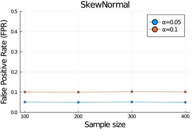
The results of FPRs, TPRs and CIs are shown in Fig. 2(a), (b) and (c), respectively. The FPRs and TPRs were estimated by 100 trials, and the plots in Fig. 2 (a) and (b) are the averages when the 100 trials were repeated 20 times for FPR and 10 times for TPR, whereas the plots in Fig. 2(c) are the results of 100 trials. In both methods, the FPRs are properly controlled under the significance level . Regarding the TPR comparison, it is obvious that Homotopy method has the higher power than Quadratic because it is minimally conditioned. The results of the CIs are consistent with the results of TPRs.

(a) False Positive Rates (FPRs)

(b) True Positive Rates (TPRs)

(c) Confidence Interval (CI) Lengths
Real data experiments
We compared the proposed method (Homotopy) and conventional method (Quadratic) on the same three real datasets.From each of the original dataset, we randomly generated sub-sampled datasets with sizes 25, 50 and 100. We applied the proposed and the conventional methods to each sub-sampled dataset, examined the cases where the selective -values of a selected feature was different between the two methods, and computed the percentage of times when the proposed method provided smaller selective -values than the conventional one. Table 2 shows the results from 1000 trials. The proposed method provides smaller selective -values than the conventional method significantly more frequently especially when is large.
6 Conclusion
In this paper, we proposed a more powerful and general conditional SI method for SFS algorithm. We resolved the over-conditioning problem in existing approaches by introducing the homotopy continuation approach. The experimental results indicated that the proposed homotopy-based approach is more powerful and general.
Acknowledgement
This work was partially supported by MEXT KAKENHI (20H00601, 16H06538), JST CREST (JPMJCR1502), RIKEN Center for Advanced Intelligence Project, and RIKEN Junior Research Associate Program.
Appendix A Proofs
A.1 Proof of Lemma 1
Proof.
Let for all and write and . By conditioning on the histories ,
for all such that . This indicates that
| (18) |
for all and such that , where is the sequence of the selected features when the -step SFS algorithm is applied to the response vector . By further conditioning on the signs , (18) is written as
for all and such that and . By restricting on a line , the range of is written as
| (19) |
∎
A.2 The proof of Lemma 2
Proof.
For a set of features and a response vector in a line, let us denote the AIC as a function of and as . Subsequently, by substituting into (14), it is written as a quadratic function of as
| (20) |
Equation (20) represents the range of such that when is fed into the algorithm, the same history is obtained. Let the sequence of the selected models corresponding to the history be
where is the number of steps in the history . Next, the event of the history can be fully characterized by comparing AICs as follows:
| (21) |
for and
| (22) |
Here, the first and second inequalities in (21) indicate that the selected model at step has the smallest AIC among all possible choices, the third inequality in (21) indicates that the AIC of the selected model at step is smaller than that at the previous step, and two inequalities (22) indicate that the AIC of the selected model at the final step cannot be decreased anymore. Because the AIC is written as a quadratic function of as in (20) under the fixed history , all these conditions are written as quadratic inequalities of . This means that the range of that satisfies these conditions is represented by a finite set of quadratic inequalities of . ∎
Appendix B Details of Experiments
We executed the experiments on Intel(R) Xeon(R) CPU E5-2687W v3 @ 3.10GHz.
Comparison methods in the case of Forward SFS.
In the case of forward SFS, we remind that results a set of selected featured when applying forward SFS algorithm to . With a slight abuse of notations, let and respectively denote the history and signs obtained when applying algorithm to . We compared the following five methods:
-
•
Homotopy: conditioning on the selected features (minimal conditioning), i.e.,
-
•
Homotopy-H: additionally conditioning on the history , i.e.,
Here, we note that already includes the event .
-
•
Homotopy-S: additionally conditioning on the signs, i.e.,
-
•
Polytope (Tibshirani et al., 2016): additionally conditioning on both history and signs , i.e.,
This definition is equivalent to
where is defined in §3.
-
•
DS: data splitting is the commonly used procedure for the purpose of selection bias correction. In this approach, the data is randomly divided in two halves — first half used for model selection and the other for inference.
Comparison methods in the case of Forward-Backward SFS.
In the case of forward-backward SFS, results a set of selected featured when applying forward-backward SFS algorithm to , and results the history. We compared the following two methods:
-
•
Homotopy: conditioning on the selected features (minimal conditioning), i.e.,
-
•
Quadratic: additionally conditioning on the history (implemented by using quadratic inequality-based conditional SI in (Loftus and Taylor, 2015)), i.e.,
Definition of TPR.
In SI, we only conduct statistical testing when there is at least one hypothesis discovered by the algorithm. Therefore, the definition of TPR, which can be also called conditional power, is as follows:
where is the number of truly positive features selected by the algorithm (e.g., SFS) and is the number of truly positive features whose null hypothesis is rejected by SI.
Demonstration of confidence interval (forward SFS).
We generated outcomes as , where and . We set , and . We note that the number of selected features between the four options of conditional SI methods (Homotopy, Homotopy-H, Homotopy-S, Polytope) and DS can be different. Therefore, for a fair comparison, we only consider the features that are selected in both cases. Figure 3 shows the demonstration of CIs for each selected feature. The results are consistent with Fig. 1 (b).

Appendix C Experiments on Computational Aspects (Forward SFS)
We demonstrate the computational efficiency of the proposed Homotopy method. We generated outcomes as , where and . We set and . In Figure 4, we show the results of comparing the computational time between the proposed Homotopy method and the existing method. For the existing study, if we want to keep high statistical power, we have to enumerate a huge number of all the combinations of histories and signs which is only feasible when the number of selected features is fairly small. We observe in blue plots in Fig. 4 that the computational cost of existing method is exponentially increasing with the number of selected features. With the proposed method, we are able to significantly reduce the computational cost while keeping high power.

One might wonder how we can circumvent the computational bottleneck of exponentially increasing number of polytopes. Our experience suggests that, by focusing on the line along the test-statistic in data space, we can skip majority of the polytopes that do not affect the truncated Normal sampling distribution because they do not intersect with this line. In other words, we can skip majority of combinations of histories and signs that never appear. We show the violin plot of the actual numbers of intervals of the test statistic that involves in the construction of truncated sampling distribution in Figure 5. Here, we set and . Regarding Homotopy and Homotopy-S, the number of polytopes linearly increases when increasing . This is the reason why our method is highly efficient. In regard to Homotopy-H, the number of polytopes decreases because the history constraint is too strict when is increased.

Appendix D Experiments on Robustness (Forward-Backward SFS)
We applied our proposed method to the cases where the noise follows Laplace distribution, skew normal distribution (skewness coefficient 10), and distribution. We also conducted experiments when was also estimated from the data. We generated outcomes as , , where , and follows Laplace distribution, skew normal distribution, or distribution with zero mean and standard deviation was set to 1. In the case of estimated , . We set all elements of to 0, and set . For each case, we ran 1,200 trials for each . The FPR results are shown in Figure 6. Although we only demonstrate the results for the case of forward-backward SFS algorithm, the extension to forward SFS algorithm with similar setting is straightforward.


Appendix E Homotopy-based SI for Cross-Validation (Forward SFS)
In this section, we introduce a method for SI conditional also on the selection of the number of selected features via cross-validation. Consider selecting the number of steps in the SFS method from a given set of candidates where is the number of candidates. When conducting cross-validation on the observed dataset , suppose that is the event that is selected as the best one. The test-statistic for the selected feature when applying the SFS method with steps to is then defined as
| (23) |
We note that and depend on but we omit the dependence for notational simplicity. The conditional data space in (9) with the event of selecting is then written as
| (24) |
where . The truncation region can be obtained by the intersection of the following two sets:
Since the former can be obtained by using the method described in §3, the remaining task is to identify the latter .
For notational simplicity, we consider the case where the dataset is divided into training and validation sets, and the latter is used for selecting . The following discussion can be easily extended to cross-validation scenario. Let us re-write
With a slight abuse of notation, for , let be the set of selected features by applying -step SFS method to . The validation error is then defined as
| (25) |
where . Then, we can write
Since the validation error in (25) is a picecewise-quadratic function of , we have a corresponding picecewise-quadratic function of for each . The truncation region can be identified by the intersection of the intervals of in which the validation error corresponding to is minimum among a set of picecewise-quadratic functions for all the other .
Loftus (2015) already discussed that it is possible to consider cross-validation event into conditional SI framework. However, his method is highly over-conditioned in the sense that additional conditioning on all intermediate models in the process of cross-validation is required. Our method described above is minimumly-conditioned SI in the sense that our inference is conducted based exactly on the conditional sampling distribution of the test-statistic in (23) without any extra conditions.
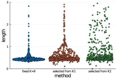
For the experiments on cross-validation, we demonstrate the TPRs and the CIs between the cases when is fixed and is selected from the set , or using -fold cross-validation. We set , only the first elements of was set to , and all the rest were set to . We show that the TPR tends to decrease when increasing the size of in Figure 7. This is due to the fact that when we increase the size of , we have to condition on more information which leads to shorter truncation interval and results low TPR. The TPR results are consistent with the CI results shown in Figure 8. In other words, when increasing the size of , the lower the TPR is, the longer the length of CI becomes.

References
- Lee et al. (2016) Jason D Lee, Dennis L Sun, Yuekai Sun, Jonathan E Taylor, et al. Exact post-selection inference, with application to the lasso. The Annals of Statistics, 44(3):907–927, 2016.
- Tibshirani et al. (2016) Ryan J Tibshirani, Jonathan Taylor, Richard Lockhart, and Robert Tibshirani. Exact post-selection inference for sequential regression procedures. Journal of the American Statistical Association, 111(514):600–620, 2016.
- Fithian et al. (2014) William Fithian, Dennis Sun, and Jonathan Taylor. Optimal inference after model selection. arXiv preprint arXiv:1410.2597, 2014.
- Benjamini and Yekutieli (2005) Yoav Benjamini and Daniel Yekutieli. False discovery rate–adjusted multiple confidence intervals for selected parameters. Journal of the American Statistical Association, 100(469):71–81, 2005.
- Leeb and Pötscher (2005) Hannes Leeb and Benedikt M Pötscher. Model selection and inference: Facts and fiction. Econometric Theory, pages 21–59, 2005.
- Leeb et al. (2006) Hannes Leeb, Benedikt M Pötscher, et al. Can one estimate the conditional distribution of post-model-selection estimators? The Annals of Statistics, 34(5):2554–2591, 2006.
- Benjamini et al. (2009) Yoav Benjamini, Ruth Heller, and Daniel Yekutieli. Selective inference in complex research. Philosophical Transactions of the Royal Society A: Mathematical, Physical and Engineering Sciences, 367(1906):4255–4271, 2009.
- Pötscher et al. (2010) Benedikt M Pötscher, Ulrike Schneider, et al. Confidence sets based on penalized maximum likelihood estimators in gaussian regression. Electronic Journal of Statistics, 4:334–360, 2010.
- Berk et al. (2013) Richard Berk, Lawrence Brown, Andreas Buja, Kai Zhang, Linda Zhao, et al. Valid post-selection inference. The Annals of Statistics, 41(2):802–837, 2013.
- Lockhart et al. (2014) Richard Lockhart, Jonathan Taylor, Ryan J Tibshirani, and Robert Tibshirani. A significance test for the lasso. Annals of statistics, 42(2):413, 2014.
- Taylor et al. (2014) Jonathan Taylor, Richard Lockhart, Ryan J Tibshirani, and Robert Tibshirani. Post-selection adaptive inference for least angle regression and the lasso. arXiv preprint arXiv:1401.3889, 354, 2014.
- Fithian et al. (2015) William Fithian, Jonathan Taylor, Robert Tibshirani, and Ryan Tibshirani. Selective sequential model selection. arXiv preprint arXiv:1512.02565, 2015.
- Choi et al. (2017) Yunjin Choi, Jonathan Taylor, Robert Tibshirani, et al. Selecting the number of principal components: Estimation of the true rank of a noisy matrix. The Annals of Statistics, 45(6):2590–2617, 2017.
- Tian et al. (2018) Xiaoying Tian, Jonathan Taylor, et al. Selective inference with a randomized response. The Annals of Statistics, 46(2):679–710, 2018.
- Chen and Bien (2019) Shuxiao Chen and Jacob Bien. Valid inference corrected for outlier removal. Journal of Computational and Graphical Statistics, pages 1–12, 2019.
- Hyun et al. (2018) Sangwon Hyun, Kevin Lin, Max G’Sell, and Ryan J Tibshirani. Post-selection inference for changepoint detection algorithms with application to copy number variation data. arXiv preprint arXiv:1812.03644, 2018.
- Loftus and Taylor (2014) Joshua R Loftus and Jonathan E Taylor. A significance test for forward stepwise model selection. arXiv preprint arXiv:1405.3920, 2014.
- Loftus and Taylor (2015) Joshua R Loftus and Jonathan E Taylor. Selective inference in regression models with groups of variables. arXiv preprint arXiv:1511.01478, 2015.
- Panigrahi et al. (2016) Snigdha Panigrahi, Jonathan Taylor, and Asaf Weinstein. Bayesian post-selection inference in the linear model. arXiv preprint arXiv:1605.08824, 28, 2016.
- Yang et al. (2016) Fan Yang, Rina Foygel Barber, Prateek Jain, and John Lafferty. Selective inference for group-sparse linear models. In Advances in Neural Information Processing Systems, pages 2469–2477, 2016.
- Suzumura et al. (2017) Shinya Suzumura, Kazuya Nakagawa, Yuta Umezu, Koji Tsuda, and Ichiro Takeuchi. Selective inference for sparse high-order interaction models. In Proceedings of the 34th International Conference on Machine Learning-Volume 70, pages 3338–3347. JMLR. org, 2017.
- Tanizaki et al. (2020) Kosuke Tanizaki, Noriaki Hashimoto, Yu Inatsu, Hidekata Hontani, and Ichiro Takeuchi. Computing valid p-values for image segmentation by selective inference. 2020.
- Duy et al. (2020a) Vo Nguyen Le Duy, Hiroki Toda, Ryota Sugiyama, and Ichiro Takeuchi. Computing valid p-value for optimal changepoint by selective inference using dynamic programming. arXiv preprint arXiv:2002.09132, 2020a.
- Terada and Shimodaira (2019) Yoshikazu Terada and Hidetoshi Shimodaira. Selective inference after variable selection via multiscale bootstrap. arXiv preprint arXiv:1905.10573, 2019.
- Liu et al. (2018) Keli Liu, Jelena Markovic, and Robert Tibshirani. More powerful post-selection inference, with application to the lasso. arXiv preprint arXiv:1801.09037, 2018.
- Duy and Takeuchi (2020) Vo Nguyen Le Duy and Ichiro Takeuchi. Parametric programming approach for powerful lasso selective inference without conditioning on signs. arXiv preprint arXiv:2004.09749, 2020.
- Osborne et al. (2000) Michael R Osborne, Brett Presnell, and Berwin A Turlach. A new approach to variable selection in least squares problems. IMA journal of numerical analysis, 20(3):389–403, 2000.
- Efron and Tibshirani (2004) B. Efron and R. Tibshirani. Least angle regression. Annals of Statistics, 32(2):407–499, 2004.
- Hastie et al. (2004) T. Hastie, S. Rosset, R. Tibshirani, and J. Zhu. The entire regularization path for the support vector machine. Journal of Machine Learning Research, 5:1391–415, 2004.
- Rosset and Zhu (2007) S. Rosset and J. Zhu. Piecewise linear regularized solution paths. Annals of Statistics, 35:1012–1030, 2007.
- Bach et al. (2006) F. R. Bach, D. Heckerman, and E. Horvits. Considering cost asymmetry in learning classifiers. Journal of Machine Learning Research, 7:1713–41, 2006.
- Tsuda (2007) K. Tsuda. Entire regularization paths for graph data. In In Proc. of ICML 2007, pages 919–925, 2007.
- Lee and Scott (2007) G. Lee and C. Scott. The one class support vector machine solution path. In Proc. of ICASSP 2007, pages II521–II524, 2007.
- Takeuchi et al. (2009) I. Takeuchi, K. Nomura, and T. Kanamori. Nonparametric conditional density estimation using piecewise-linear solution path of kernel quantile regression. Neural Computation, 21(2):539–559, 2009.
- Takeuchi and Sugiyama (2011) Ichiro Takeuchi and Masashi Sugiyama. Target neighbor consistent feature weighting for nearest neighbor classification. In Advances in neural information processing systems, pages 576–584, 2011.
- Karasuyama and Takeuchi (2010) M. Karasuyama and I. Takeuchi. Nonlinear regularization path for quadratic loss support vector machines. IEEE Transactions on Neural Networks, 22(10):1613–1625, 2010.
- Hocking et al. (2011) T. Hocking, j. P. Vert, F. Bach, and A. Joulin. Clusterpath: an algorithm for clustering using convex fusion penalties. In Proceedings of the 28th International Conference on Machine Learning, pages 745–752, 2011.
- Karasuyama et al. (2012) M. Karasuyama, N. Harada, M. Sugiyama, and I. Takeuchi. Multi-parametric solution-path algorithm for instance-weighted support vector machines. Machine Learning, 88(3):297–330, 2012.
- Ogawa et al. (2013) Kohei Ogawa, Motoki Imamura, Ichiro Takeuchi, and Masashi Sugiyama. Infinitesimal annealing for training semi-supervised support vector machines. In International Conference on Machine Learning, pages 897–905, 2013.
- Takeuchi et al. (2013) Ichiro Takeuchi, Tatsuya Hongo, Masashi Sugiyama, and Shinichi Nakajima. Parametric task learning. Advances in Neural Information Processing Systems, 26:1358–1366, 2013.
- Duy et al. (2020b) Vo Nguyen Le Duy, Shogo Iwazaki, and Ichiro Takeuchi. Quantifying statistical significance of neural network representation-driven hypotheses by selective inference. arXiv preprint arXiv:2010.01823, 2020b.