Moral Machine or Tyranny of the Majority?

Michael Feffer Carnegie Mellon University
{mfeffer, hheidari, zlipton}@andrew.cmu.edu Hoda Heidari¹¹1These authors contributed equally. Carnegie Mellon University
{mfeffer, hheidari, zlipton}@andrew.cmu.edu Zachary C. Lipton¹¹footnotemark: 1 Carnegie Mellon University
{mfeffer, hheidari, zlipton}@andrew.cmu.edu

Abstract

With Artificial Intelligence systems increasingly applied in consequential domains, researchers have begun to ask how these systems ought to act in ethically charged situations where even humans lack consensus. In the Moral Machine project, researchers crowdsourced answers to “Trolley Problems” concerning autonomous vehicles. Subsequently, Noothigattu et al. (2018) proposed inferring linear functions that approximate each individual’s preferences and aggregating these linear models by averaging parameters across the population. In this paper, we examine this averaging mechanism, focusing on fairness concerns in the presence of strategic effects. We investigate a simple setting where the population consists of two groups, with the minority constituting an $\alpha<0.5$ share of the population. To simplify the analysis, we consider the extreme case in which within-group preferences are homogeneous. Focusing on the fraction of contested cases where the minority group prevails, we make the following observations: (a) even when all parties report their preferences truthfully, the fraction of disputes where the minority prevails is less than proportionate in $\alpha$ ; (b) the degree of sub-proportionality grows more severe as the level of disagreement between the groups increases; (c) when parties report preferences strategically, pure strategy equilibria do not always exist; and (d) whenever a pure strategy equilibrium exists, the majority group prevails 100% of the time. These findings raise concerns about stability and fairness of preference vector averaging as a mechanism for aggregating diverging voices. Finally, we discuss alternatives, including randomized dictatorship and median-based mechanisms.

1 Introduction

Machine learning (ML) has increasingly been employed to automate decisions in consequential domains including autonomous vehicles, healthcare, hiring, finance, and criminal justice. These domains present many ethically charged decisions, where even knowledgeable humans may lack consensus about the right course of action. Consequently, AI researchers have been forced to consider how to resolve normative disputes when competing values come into conflict. The formal study of such ethical quandaries long predates the advent of modern AI systems. For example, philosophers have long debated Trolley Problems [32], which generally take the form of inescapable decisions among normatively undesirable alternatives. Notably, these problems typically lack clear-cut answers, and people’s judgments are often sensitive to subtle details in the provided context.

Questions about whose values are represented and what objectives are optimized in ML-based systems have become especially salient in light of documented instances of algorithmic bias in deployed systems [1, 4, 26]. Faced with questions of whose values ought to prevail when a judgment must be made, some AI ethics researchers have advocated participatory machine learning, a family of methods for democratizing decisions by incorporating the views of a variety of stakeholders [22, 16, 18]. For example, a line of papers on preference elicitation tasks stakeholders with choosing among sets of alternatives [16, 22, 18, 14, 13, 10]. In many of these studies, the hope is to compute a socially aligned objective function [22, 10] or fairness metric [16, 13, 14].

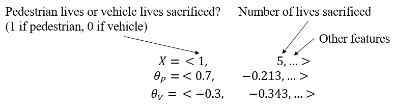
In a pioneering study, Awad et al. [2] introduced the Moral Machine, a large-scale crowdsourcing study in which millions of participants from around the world were presented with autonomous driving scenarios in the style of Trolley Problems. Participants were shown images depicting two possible outcomes and asked which alternative they preferred. In one scenario, the first alternative might be to collide with a barrier and sacrifice several young passengers, and the second to pulverize two elderly pedestrians in a crosswalk. Utilizing the Moral Machine dataset, Noothigattu et al. [25] proposed methods for inferring each participant’s preferences. Specifically, they represent each alternative by a fixed-length vector of attributes, $\mathbf{x}$ , and each participant’s scoring function as the dot product between their preference vector $\boldsymbol{\theta}$ and the alternative $\mathbf{x}$ . The objective is to infer parameters $\boldsymbol{\theta}$ so that whenever an individual prefers one alternative over another, the preferred alternative receives a higher score. To aggregate these preference vectors across a population, Noothigattu et al. [25] propose to simply average them. Faced with a “moral dilemma”, an autonomous vehicle would conceivably featurize each alternative, compute their dot products with the aggregate preference vector, and choose the highest scoring option. These approaches have been echoed in a growing body of follow-up studies [28, 33, 19]. However, despite the work’s influence, key properties of the proposed mechanism remain under-explored.

In this paper, we analyze the mechanism of averaging preference vectors across a population, focusing on stability, strategic effects, and implications for fairness. While averaging mechanisms have been extensively studied [15, 29, 23, 30], Noothigattu et al. [25]’s approach warrants analysis for several reasons: (i) here, individuals vote on the parameters of a ranking algorithm, rather than directly on the outcomes of interest and (ii) since only the ordering induced by the preference vectors matters, only the direction of the aggregate vector is relevant. We introduce a stylized model in which the population of interest consists of a (disadvantaged) minority group, constituting an $\alpha<0.5$ share of the population, and an (advantaged) majority group constituting $1-\alpha$ . The goal is to determine how an autonomous vehicle should behave by polling the population via Noothigattu et al. [25]’s algorithm, where the problem setup is identical to that of the Moral Machine [2]. Because we only observe which alternative an individual prefers, our analysis focuses on the fraction of cases (among disputed cases) where each group prevails.

To clarify the fairness properties of the mechanism, we concentrate our analysis on an stylized setting in which within-group preferences are homogeneous. We emphasize this assumption is only meant for simplifying the analysis and revealing fundamental limitations of the simple preference vector averaging mechanism. The problems we identify here do not simply disappear in more complicated settings with within-group variation in preferences. Moreover, to isolate the role of the aggregation mechanism, we assume participants can directly report their preference vectors. With these assumptions in place, our analysis makes the following key observations: (i) even when preferences are reported truthfully, the fraction of cases where the minority prevails is sub-proportionate (i.e., less than $\alpha$ ); (ii) the degree of sub-proportionality grows more severe when the divergence between the two groups’ preference vectors is large; (iii) as with most averaging-based approaches, this mechanism is not strategy-proof; (iv) whenever a pure strategy equilibrium exists, the majority group prevails on 100% of cases; and (v) last but not least, while other stable and incentive-compatible mechanisms do exist (e.g., the randomized dictatorship model), they come with other fundamental shortcomings.

Several takeaways flow from our analysis. First, this averaging of preference vectors is qualitatively different from averaging votes directly on outcomes of interest, giving rise to instability and surprising strategic behavior. Second, the degree of compromise among majority and minority demographics, both under truthful and strategic settings, is an important consideration when designing aggregation mechanisms to support participatory ML systems. Finally, our work raises critical questions regarding the limitations of simple voting methods to ensure stakeholders’ participation in the design of high-stakes automated decision-making systems. We hope that this work encourages the community to reflect on the importance of addressing normative disagreements among stakeholders—not simply by passing them through an aggregation mechanism, but by effectively giving voice to the disadvantaged communities and facilitating deliberations necessary to reach an acceptable outcome for all stakeholders.

2 Related Work

Our work draws on the preference elicitation and computational social choice literatures. We build most directly on a line of work consisting of the Moral Machine [2] and subsequently proposed procedures for inferring and aggregating preferences [25]. These studies inspired numerous follow-up articles, such as Pugnetti & Schläpfer [28], who pose the same questions to Swiss vehicle customers; Wang et al. [33], who modify the algorithms to support differential privacy; and Kemmer et al. [19], who evaluate various methods of aggregating crowdsourced judgments, including averaging.

Preference elicitation for participatory ML

Lee et al. [22] helped nonprofit volunteers build ML algorithms via pairwise comparisons and aggregating the resulting preferences using Borda Count voting. Johnston et al. [17] adopted participatory mechanisms to determine how to allocate COVID-19 triage supplies. Freedman et al. [10] modified parameter weights in their kidney exchange linear programs to help break ties based on inferred participant preferences about who should receive kidney donations. Still other works that learn fairness metrics from user input assume a single participant or a group capable of coming to consensus, and therefore employ no aggregation mechanism [16, 13, 14]. Note that, per Chamberlin [5], that using Borda Count instead of averaging does not necessarily alleviate issues related to strategic voting. Similarly, a minimax group regret approach as employed in Johnston et al. [17] may also be vulnerable to subgroup strategic voting.

Computational Social Choice

Like us, El-Mhamdi et al. [9] highlights the general susceptibility of averaging-based methods to strategic voting and discusses alternative median-based mechanisms. While they mention the Moral Machine as an example, they do not analyze the particular mechanism presented in [25] or provide any of the insights about fairness and strategic concerns presented in our work. Moulin [24], Conitzer et al. [7], Zhang et al. [35] propose median-based algorithms for voting in a strategy-proof manner in the context of crowdsourcing societal tradeoffs. Brill & Conitzer [3] address strategic voting, noting that median-based approaches are less susceptible to manipulation. Conitzer et al. [6] describes issues with crowdsourcing societal tradeoffs more generally. Concerning randomized dictatorship models, Gibbard [11, 12] introduce randomized solutions as “unattractive” yet strategy-proof approaches. Zeckhauser [34] similarly states that randomized dictatorship has some favorable characteristics in that it forces voters to report their true preferences (i.e., is strategy-proof) and is probabilistically linear (i.e., switching votes from one alternative to another only affects the selection probabilities of those two alternatives in a linear fashion). Instead of proposing other aggregation mechanisms, both Landemore & Page [21] and Pierson [27] argue that deliberation and discussion among participants are procedures that, when used in conjunction with voting, can lead to better outcomes than voting as a standalone process.

3 Our Problem Setup

Consider a population consisting of two groups: A, the majority, and D, a minority constituting $\alpha<0.5$ fraction of the population. Each group is characterized by a true preference vector $\boldsymbol{\theta}^{*}_{i}\in\mathbb{R}^{d}$ that determines the preferences of all members of that group over outcomes/alternatives. (In the autonomous vehicle example, the outcome could be the individuals chosen to be saved in face of an unavoidable accident.) Each alternative is represented by a feature vector $\mathbf{x}\in\mathbb{R}^{d}$ . We assume alternatives are drawn independently from $M$ , a spherically symmetric distribution centered at the origin with radius 1. Members of group $i$ prefer alternative $\mathbf{x}\in\mathbb{R}^{d}$ to alternative $\mathbf{y}\in\mathbb{R}^{d}$ whenever $\boldsymbol{\theta}^{*}_{i}.\mathbf{x}\geq\boldsymbol{\theta}^{*}_{i}.\mathbf{y}$ , i.e., whenever $\boldsymbol{\theta}^{*}_{i}.(\mathbf{x}-\mathbf{y})\geq 0$ . So the true preference vector $\boldsymbol{\theta}^{*}_{i}\in\mathbb{R}^{d}$ of group $i\in\{A,D\}$ allows us to calculate their rankings over any set of alternatives. See Appendix A for a concrete example of such vectors. Throughout and unless otherwise specified, we assume $\boldsymbol{\theta}^{*}_{A}\neq\boldsymbol{\theta}^{*}_{D}$ (e.g., in the context of the Moral Machine experiment, $\boldsymbol{\theta}^{*}_{A}$ may reflect group A’s preference for sacrificing pedestrians when an autonomous vehicle is faced with an accident, and $\boldsymbol{\theta}^{*}_{D}$ reflects group D’s preference for sacrificing passengers).

Note that in enforcing within-group homogeneity of preferences in our model, we do not assert that groups are homogeneous in the real world. Rather, our aim is to elucidate whether this mechanism respects the preferences of minority groups. In other words, the homogeneity assumption allows us to make a clear analytic point rather than state a realistic or normatively desirable situation. Such simplifying assumptions are common in economics and theoretical computer science literature (e.g., Costinot & Kartik [8], Krishna & Morgan [20]).

Formulation as a game

We consider a two-player normal-form game $G={(S_{A},u_{A}),(S_{D},u_{D})}$ in which groups in the setup described above correspond to players, $A$ and $D$ (so player $A$ and $D$ have true preference vectors $\boldsymbol{\theta}^{*}_{A}$ and $\boldsymbol{\theta}^{*}_{D}$ , respectively). $S_{i}$ denotes player $i$ ’s strategy space, and $u_{i}$ their payoff/utility. More precisely, each player $i\in\{A,D\}$ strategically reports a preference vector $\boldsymbol{\theta}_{i}\in S_{i}$ (which may be different from $\boldsymbol{\theta}^{*}_{i}$ ), where $S_{i}$ consists of all $d$ -dimensional vectors with Euclidean norm equal to 1. The payoff function for player $i$ , $u_{i}:\mathbb{R}^{d}\times\mathbb{R}^{d}\longrightarrow\mathbb{R}$ , is a function where $u_{i}(\boldsymbol{\theta}_{A},\boldsymbol{\theta}_{D})$ indicates the payoff of player $i\in\{A,D\}$ when players $A$ and $D$ report preference vectors $\boldsymbol{\theta}_{A}$ and $\boldsymbol{\theta}_{D}$ , respectively. We assume the payoff function for each player $i\in\{A,D\}$ captures the proximity of their true preference vector $\boldsymbol{\theta}^{*}_{i}$ to the aggregate vector, $\boldsymbol{\theta}_{C}$ , obtained by a simple averaging mechanism: $\boldsymbol{\theta}_{C}=(\alpha\boldsymbol{\theta}_{D}+(1-\alpha)\boldsymbol{\theta}_{A})/{\lVert\alpha\boldsymbol{\theta}_{D}+(1-\alpha)\boldsymbol{\theta}_{A}\rVert}$ .²²2While only the direction of $\boldsymbol{\theta}_{C}$ matters, we normalize its length for mathematical convenience.

Each player aims to maximize the fraction of decisions that agree with their true preferences. As shown in Proposition 1, achieving this goal requires that each player $i\in\{A,D\}$ reports a preference vector such that the resulting aggregate vector $\boldsymbol{\theta}_{C}$ is closest, as measured by cosine similarity, to their true preference vector $\boldsymbol{\theta}^{*}_{i}$ . To show this formally, we first define the notion of agreement between two preference vectors.

Definition 1.

Consider two preference vectors $\boldsymbol{\theta}_{i}$ and $\boldsymbol{\theta}_{j}\in\mathbb{R}^{d}$ and a spherically symmetric distribution $M$ over the space of all alternatives (i.e., $\mathbb{R}^{d}$ ). The level of agreement between $\boldsymbol{\theta}_{i}$ and $\boldsymbol{\theta}_{j}$ , denoted by $\rho(\boldsymbol{\theta}_{i},\boldsymbol{\theta}_{j})$ , is the probability, over draws of pairs of alternatives from $M$ , such that $\boldsymbol{\theta}_{i}$ and $\boldsymbol{\theta}_{j}$ rank the alternatives in the same order:

\rho(\boldsymbol{\theta}_{i},\boldsymbol{\theta}_{j})=\mathbb{P}_{\mathbf{x}\sim M,\mathbf{y}\sim M}\left[\mathrm{sign}({\boldsymbol{\theta}_{i}}\cdot(\mathbf{y}-\mathbf{x}))=\mathrm{sign}({\boldsymbol{\theta}_{j}}\cdot(\mathbf{y}-\mathbf{x}))\right].

Proposition 1.

Suppose alternatives are sampled i.i.d. from a spherically symmetric distribution $M$ defined over $\mathbb{R}^{d}$ . Then for any two preference vectors $\boldsymbol{\theta}_{i},\boldsymbol{\theta}_{j}\in\mathbb{R}^{d}$ ,

\rho(\boldsymbol{\theta}_{i},\boldsymbol{\theta}_{j})=\frac{\pi-\cos^{-1}{(\boldsymbol{\theta}_{i}\cdot\boldsymbol{\theta}_{j}})}{\pi}.

Proof.

Note that the preference of a player $i$ over alternatives $\mathbf{x}$ and $\mathbf{y}$ depends only on the sign of $\boldsymbol{\theta}_{i}\cdot(\mathbf{y}-\mathbf{x})$ . Because $\mathbf{x}$ and $\mathbf{y}$ are drawn independently from a spherically symmetrical distribution $M$ , we can see, by symmetry, that the difference vector, $\mathbf{y}-\mathbf{x}$ , can points in any direction from $[0,2\pi]$ with equal (uniform) probability.

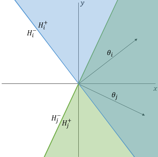
Any preference vector $\boldsymbol{\theta}$ defines two half-spaces over the vector $\mathbf{y}-\mathbf{x}\in\mathbb{R}^{d}$ . By $H^{+}$ , we denote the half-space in which $\boldsymbol{\theta}\cdot(\mathbf{y}-\mathbf{x})>0$ (and thus $\mathbf{y}$ is preferred to $\mathbf{x}$ ) and by $H^{-}$ , we denote the half-space in which $\boldsymbol{\theta}\cdot(\mathbf{y}-\mathbf{x})<0$ (and thus $\mathbf{x}$ is preferred to $\mathbf{y}$ ). Because the event where $\mathbf{x}=\mathbf{y}$ has $0$ measure, tie-breaking conventions will not impact our analysis.

Note that for any given player, the line separating $H^{+}$ from $H^{-}$ is perpendicular to $\boldsymbol{\theta}$ and passes through the origin. Disagreements among $\boldsymbol{\theta}_{i}$ and $\boldsymbol{\theta}_{j}$ correspond to pairs of alternatives such that either $\mathbf{x}-\mathbf{y}\in\{H_{j}^{-}\cap H_{i}^{+}\}$ or $\mathbf{x}-\mathbf{y}\in\{H_{i}^{-}\cap H_{j}^{+}\}$ . So we have:

	$\displaystyle\rho(\boldsymbol{\theta}_{i},\boldsymbol{\theta}_{j})$	$\displaystyle=$	$\displaystyle\mathbb{P}_{\mathbf{x}\sim M,\mathbf{y}\sim M}\left[\mathrm{sign}({\boldsymbol{\theta}_{i}}\cdot(\mathbf{y}-\mathbf{x}))=\mathrm{sign}({\boldsymbol{\theta}_{j}}\cdot(\mathbf{y}-\mathbf{x}))\right],$
		$\displaystyle=$	$\displaystyle 1-\mathbb{P}_{\mathbf{x}\sim M,\mathbf{y}\sim M}\left[\mathbf{x}-\mathbf{y}\in H_{j}^{-}\cap H_{i}^{+}\text{ or }\mathbf{x}-\mathbf{y}\in H_{j}^{+}\cap H_{i}^{-}\right].$

Note that both $\{H_{j}^{-}\cap H_{i}^{+}\}$ and $\{H_{i}^{-}\cap H_{j}^{+}\}$ are cones whose vertices lie at the origin and whose vertex angles are each given by $\measuredangle(\boldsymbol{\theta}_{i},\boldsymbol{\theta}_{j})$ . See Figure 1 for an illustration of these half-spaces and their intersections.

Refer to caption — Figure 1: Half-spaces $H_{i}^{+},H_{i}^{-},H_{j}^{+},H_{j}^{-}$ and intersections for preference vectors $\boldsymbol{\theta}_{i}$ and $\boldsymbol{\theta}_{j}$ .

Because the alternatives, $\mathbf{x},\mathbf{y}$ are drawn i.i.d. from a spherically symmetric distribution,

	$\displaystyle\mathbb{P}\left[\mathbf{x}-\mathbf{y}\in\{H_{j}^{-}\cap H_{i}^{+}\}\right]$	$\displaystyle=\mathbb{P}\left[\mathbf{x}-\mathbf{y}\in\{H_{i}^{-}\cap H_{j}^{+}\}\right]$
		$\displaystyle=\frac{\cos^{-1}(\boldsymbol{\theta}_{i}\cdot\boldsymbol{\theta}_{j})}{2\pi}.$

Moreover, because these regions of disagreement are disjoint, the total probability of disagreement $\boldsymbol{\theta}_{i}$ , $\boldsymbol{\theta}_{j}$ is given by the sum of the probabilities of $\mathbf{y}-\mathbf{x}$ lying in either region of disagreement, $\cos^{-1}{(\boldsymbol{\theta}_{i}\cdot\boldsymbol{\theta}_{j})})/2\pi$ . Thus, the level of agreement is given by $\frac{\pi-\cos^{-1}{(\boldsymbol{\theta}_{i}\cdot\boldsymbol{\theta}_{j})}}{\pi}.$ ∎

Because the level of agreement of the aggregate decisions with player $i$ is monotonic in the cosine similarity between their true preferences $\boldsymbol{\theta}^{*}_{i}$ and the aggregate vector $\boldsymbol{\theta}_{C}$ , we can equivalently take the cosine similarity as the payoff of interest. More precisely, we can define $u_{A},u_{D}$ as follows: for all $\boldsymbol{\theta}_{A}\in S_{A}$ and $\boldsymbol{\theta}_{D}\in S_{D}$ ,

u_{A}(\boldsymbol{\theta}_{A},\boldsymbol{\theta}_{D})=\boldsymbol{\theta}_{C}\cdot\boldsymbol{\theta}^{*}_{A},

u_{D}(\boldsymbol{\theta}_{A},\boldsymbol{\theta}_{D})=\boldsymbol{\theta}_{C}\cdot\boldsymbol{\theta}^{*}_{D}.

We are interested in understanding pure strategy Nash equilibria of the above game. To define pure strategy Nash equilibria precisely, we need to first define the concept best responses to a given pure strategy. We say a pure strategy $\boldsymbol{\theta}_{i}\in S_{i}$ is a best response to $\boldsymbol{\theta}_{-i}\in S_{-i}$ in $G$ if for all $\boldsymbol{\hat{\theta}}_{i}\in S_{i}$ ,

u_{i}(\boldsymbol{\theta}_{i},\boldsymbol{\theta}_{-i})\geq u_{i}(\boldsymbol{\hat{\theta}}_{i},\boldsymbol{\theta}_{-i}).

Given a strategy $\boldsymbol{\theta}_{-i}$ for player ${-i}$ , we will use the notation $BR_{i}(\boldsymbol{\theta}_{-i})$ to refer to the set of all pure best responses of $i$ to $\boldsymbol{\theta}_{-i}$ .

Definition 2 (Nash Equilibrium).

A strategy profile $(\boldsymbol{\theta}^{\prime}_{A},\boldsymbol{\theta}^{\prime}_{D})$ is a pure Nash Equilibrium for $G$ if $\boldsymbol{\theta}^{\prime}_{A}$ is a best-response to $\boldsymbol{\theta}^{\prime}_{D}$ and vice versa.

From here on, we restrict our analysis to the case where $d=2$ . As we argue in Appendix C, it may suffice to consider the 2-dimensional plane containing the origin, $\boldsymbol{\theta}^{*}_{A}$ , and $\boldsymbol{\theta}^{*}_{D}$ .

4 Findings

We are now ready to introduce our primary findings.

Disproportionate majority voice via the averaging mechanisms

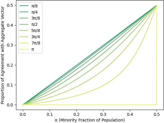
Assume that all participants truthfully report their preferences. Even here, the averaging mechanism has some strange properties. Notably, focusing on the fraction of all disputed cases where group D prevails, specifically

\mathbb{P}[\textrm{sign}({\boldsymbol{\theta}_{C}}\cdot(\mathbf{y}-\mathbf{x}))=\textrm{sign}({\boldsymbol{\theta}^{*}_{D}}\cdot(\mathbf{y}-\mathbf{x}))\>|\>\textrm{sign}({\boldsymbol{\theta}^{*}_{A}}\cdot(\mathbf{y}-\mathbf{x}))\neq\textrm{sign}({\boldsymbol{\theta}^{*}_{D}}\cdot(\mathbf{y}-\mathbf{x}))]

(1)

we find that this is sub-proportional in $\alpha$ (the pattern follows a sigmoid-like shape). Moreover, the degree of sub-proportionality depends on the angle between the true preference vectors because even though $\boldsymbol{\theta}_{C}$ is a weighted sum of $\boldsymbol{\theta}^{*}_{A}$ and $\boldsymbol{\theta}^{*}_{D}$ , the direction of $\boldsymbol{\theta}_{C}$ (and in turn the levels of agreement with the minority and majority groups) depends on the directions of $\boldsymbol{\theta}^{*}_{A}$ and $\boldsymbol{\theta}^{*}_{D}$ in addition to $\alpha$ . This can be seen clearly in Figure 2 where the probability of group D prevailing is computed via Equation 1 under varying settings of their population share $\alpha$ and for various levels of agreement between the two groups (see Appendix B). Note that sub-proportionality becomes more extreme as the angle between the true preference vectors increases.

Majority Group Can Create Aggregate Vector In Any Direction

Next, we address the setting where groups can report their preferences strategically. First, we find that for any preference vector $\boldsymbol{\theta}_{D}$ reported by the minority group, the majority group can always choose some preference vector to report such that the aggregate vector is identical to their true preferences $\boldsymbol{\theta}_{C}=\boldsymbol{\theta}^{*}_{A}$ . This implies that if a pure strategy Nash equilibrium exists, group A always gets their way. (In our running example, this implies that the autonomous vehicle always operates in accordance with group $A$ ’s preferences.)

Lemma 1.

For any fixed vector $\boldsymbol{\theta}_{D}$ played by the minority group, the majority group can report a vector $\boldsymbol{\theta}_{A}$ , such that $\boldsymbol{\theta}_{C}=\boldsymbol{\theta}^{*}_{A}$ .

Proof sketch.

In order to ensure $\boldsymbol{\theta}^{*}_{A}=\boldsymbol{\theta}_{C}$ , player $A$ must report $\boldsymbol{\theta}_{A}$ such that $\frac{\alpha\boldsymbol{\theta}_{D}+(1-\alpha)\boldsymbol{\theta}_{A}}{\lVert\alpha\boldsymbol{\theta}_{D}+(1-\alpha)\boldsymbol{\theta}_{A}\rVert}=\boldsymbol{\theta}^{*}_{A}$ . For any vector $\boldsymbol{\theta}_{D}$ , it is easy to see that the above equation is equivalent to:

\boldsymbol{\theta}_{A}=\frac{\bigg{[}\alpha(\boldsymbol{\theta}_{D}\cdot\boldsymbol{\theta}^{*}_{A})+\sqrt{\alpha^{2}(\boldsymbol{\theta}_{D}\cdot\boldsymbol{\theta}^{*}_{A})^{2}-2\alpha+1}\bigg{]}\boldsymbol{\theta}^{*}_{A}-\alpha\boldsymbol{\theta}_{D}}{(1-\alpha)}.

(2)

(See Appendix D for the full derivation.) ∎

4.1 Conditions for Pure Strategy Nash Equilibrium

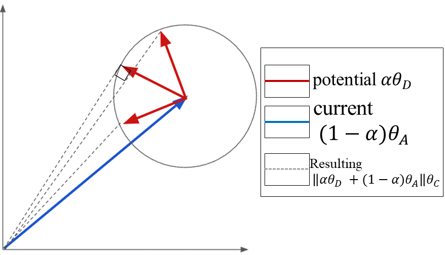
In this section, we present a necessary condition for the existence of a pure Nash Equilibrium in the above game. First, we derive the maximum amount by which the minority group can pull the aggregate vector based on their relative population size by reporting their preference strategically.

Lemma 2.

Consider a fixed reported majority group vector $\boldsymbol{\theta}_{A}$ . Suppose the minority group reports $\boldsymbol{\theta}_{D}$ to yield an aggregate vector $\boldsymbol{\theta}_{C}$ . Then for any $\boldsymbol{\theta}_{D}\in S_{D}$ ,

\measuredangle\left(\boldsymbol{\theta}_{C},\boldsymbol{\theta}_{A}\right)\leq\sin^{-1}{\left(\frac{\alpha}{1-\alpha}\right)}.

(3)

The equality occurs if and only if $\boldsymbol{\theta}_{D}$ is orthogonal to $\boldsymbol{\theta}_{C}$ .

Proof sketch.

It is easy to see that $\boldsymbol{\theta}_{D}$ yields an aggregate vector $\boldsymbol{\theta}_{C}$ such that $\measuredangle\left(\boldsymbol{\theta}_{C},\boldsymbol{\theta}_{A}\right)=\sin^{-1}{\left(\frac{\alpha\sin{(\measuredangle\left(\boldsymbol{\theta}_{C},\boldsymbol{\theta}_{D}\right))}}{1-\alpha}\right)}$ . Note that because $\sin{(\measuredangle\left(\boldsymbol{\theta}_{C},\boldsymbol{\theta}_{D}\right))}\leq 1$ , $\left(\frac{\alpha\sin{(\measuredangle\left(\boldsymbol{\theta}_{C},\boldsymbol{\theta}_{D}\right))}}{1-\alpha}\right)\leq\left(\frac{\alpha}{1-\alpha}\right)$ . Moreover, $\sin^{-1}(.)$ is a monotonic function in $[-1,1]$ . Therefore, $\measuredangle\left(\boldsymbol{\theta}_{C},\boldsymbol{\theta}_{A}\right)=\sin^{-1}{\left(\frac{\alpha\sin{(\measuredangle\left(\boldsymbol{\theta}_{C},\boldsymbol{\theta}_{D}\right))}}{1-\alpha}\right)}\leq\sin^{-1}{\left(\frac{\alpha}{1-\alpha}\right)}$ . Additionally, $\measuredangle\left(\boldsymbol{\theta}_{C},\boldsymbol{\theta}_{A}\right)=\sin^{-1}{\left(\frac{\alpha}{1-\alpha}\right)}$ if and only if $\sin{(\measuredangle\left(\boldsymbol{\theta}_{C},\boldsymbol{\theta}_{D}\right))}=1$ . This in turn happens if and only if $\boldsymbol{\theta}_{C}\perp\boldsymbol{\theta}_{D}$ .

(See Appendix E for the full derivation.) ∎

These two lemmas yield the subsequent three lemmas, which are proved in Appendix F:

First, if a pure strategy Nash equilibrium exists, the majority group can always report its preference vector such that the aggregate matches their true preferences.

Lemma 3.

Consider the game, $G$ , described in Section 3. If $(\boldsymbol{\theta}^{\prime}_{D},\boldsymbol{\theta}^{\prime}_{A})$ is a pure strategy Nash equilibrium for $G$ , then $\boldsymbol{\theta}_{C}=\boldsymbol{\theta}^{*}_{A}$ .

Second, we derive an upper bound on the angle between the aggregate and minority group’s true preferences.

Lemma 4.

For any $\boldsymbol{\theta}_{A}\in S_{A}$ , there exists $\boldsymbol{\theta}_{D}\in S_{D}$ such that $\measuredangle\left(\boldsymbol{\theta}_{C},\boldsymbol{\theta}^{*}_{D}\right)\leq\pi-\sin^{-1}\left(\frac{\alpha}{1-\alpha}\right)$ .

Lastly, in a pure strategy Nash equilibrium, the minority group’s best response is orthogonal to the aggregate.

Lemma 5.

In any pure strategy Nash equilibrium defined by best responses $\boldsymbol{\theta}^{\prime}_{A}$ and $\boldsymbol{\theta}^{\prime}_{D}$ , $\boldsymbol{\theta}^{\prime}_{D}\perp\boldsymbol{\theta}_{C}$ , and $\measuredangle\left(\boldsymbol{\theta}_{C},\boldsymbol{\theta}^{\prime}_{A}\right)=\sin^{-1}{\left(\frac{\alpha}{1-\alpha}\right)}$ .

Now, we show that a pure strategy Nash equilibrium does not always exist.

Theorem 1.

For $G$ to have a pure strategy Nash equilibrium, it must be the case that

\measuredangle\left(\boldsymbol{\theta}^{*}_{A},\boldsymbol{\theta}^{*}_{D}\right)<\pi-\sin^{-1}{\left(\frac{\alpha}{1-\alpha}\right)}.

Proof.

Suppose, via contradiction, there exists a pure strategy Nash equilibrium and $\measuredangle\left(\boldsymbol{\theta}^{*}_{A},\boldsymbol{\theta}^{*}_{D}\right)\geq\pi-\sin^{-1}{\left(\frac{\alpha}{1-\alpha}\right)}$ . Two cases are possible:

1.

$\measuredangle\left(\boldsymbol{\theta}^{*}_{A},\boldsymbol{\theta}^{*}_{D}\right)>\pi-\sin^{-1}{\left(\frac{\alpha}{1-\alpha}\right)}$ ;
2.

$\measuredangle\left(\boldsymbol{\theta}^{*}_{A},\boldsymbol{\theta}^{*}_{D}\right)=\pi-\sin^{-1}{\left(\frac{\alpha}{1-\alpha}\right)}$ .

First, consider the case where $\measuredangle\left(\boldsymbol{\theta}^{*}_{A},\boldsymbol{\theta}^{*}_{D}\right)>\pi-\sin^{-1}{\left(\frac{\alpha}{1-\alpha}\right)}$ . By Lemma 3, $\boldsymbol{\theta}^{*}_{A}=\boldsymbol{\theta}_{C}$ in this equilibrium. However, by Lemma 4, $\measuredangle\left(\boldsymbol{\theta}_{C},\boldsymbol{\theta}^{*}_{D}\right)\leq\pi-\sin^{-1}{\left(\frac{\alpha}{1-\alpha}\right)}$ given any response from the majority group. This means the minority group will report a best response $\boldsymbol{\theta}^{\prime}_{D}$ that does not yield $\boldsymbol{\theta}^{*}_{A}$ . This in turn raises a contradiction and indicates that such an equilibrium cannot exist if $\measuredangle\left(\boldsymbol{\theta}^{*}_{A},\boldsymbol{\theta}^{*}_{D}\right)>\pi-\sin^{-1}{\left(\frac{\alpha}{1-\alpha}\right)}$ .

Second, consider the case where $\measuredangle\left(\boldsymbol{\theta}^{*}_{A},\boldsymbol{\theta}^{*}_{D}\right)=\pi-\sin^{-1}{\left(\frac{\alpha}{1-\alpha}\right)}$ . By Lemma 3, $\boldsymbol{\theta}^{*}_{A}=\boldsymbol{\theta}_{C}$ in this equilibrium. Because $\boldsymbol{\theta}^{*}_{A}=\boldsymbol{\theta}_{C}$ , by Lemma 5, $\measuredangle\left(\boldsymbol{\theta}^{\prime}_{A},\boldsymbol{\theta}^{*}_{A}\right)=\left(\boldsymbol{\theta}^{\prime}_{A},\boldsymbol{\theta}_{C}\right)=\sin^{-1}{\left(\frac{\alpha}{1-\alpha}\right)}$ . Therefore $\measuredangle\left(\boldsymbol{\theta}^{\prime}_{A},\boldsymbol{\theta}^{*}_{D}\right)=\measuredangle\left(\boldsymbol{\theta}^{\prime}_{A},\boldsymbol{\theta}^{*}_{A}\right)+\measuredangle\left(\boldsymbol{\theta}^{*}_{A},\boldsymbol{\theta}^{*}_{D}\right)=\sin^{-1}{\left(\frac{\alpha}{1-\alpha}\right)}+\pi-\sin^{-1}{\left(\frac{\alpha}{1-\alpha}\right)}=\pi$ , and $\boldsymbol{\theta}^{\prime}_{A}$ is diametrically opposed to $\boldsymbol{\theta}^{*}_{D}$ . Note that there are two best responses for the minority group, both of which pull the aggregate (one by $\sin^{-1}\left(\frac{\alpha}{1-\alpha}\right)$ , the other by $-\sin^{-1}\left(\frac{\alpha}{1-\alpha}\right)$ ) towards $\boldsymbol{\theta}^{*}_{D}$ to yield $\measuredangle\left(\boldsymbol{\theta}_{C},\boldsymbol{\theta}^{*}_{D}\right)=\pi-\sin^{-1}{\left(\frac{\alpha}{1-\alpha}\right)}$ . However, only one yields $\boldsymbol{\theta}_{C}=\boldsymbol{\theta}^{*}_{A}$ . This is a contradiction because $\boldsymbol{\theta}_{C}$ does not necessarily match $\boldsymbol{\theta}^{*}_{A}$ . Therefore, this is not a pure strategy Nash equilibrium.

Thus, for $G$ to have a pure strategy Nash equilibrium, $\measuredangle\left(\boldsymbol{\theta}^{*}_{A},\boldsymbol{\theta}^{*}_{D}\right)<\pi-\sin^{-1}{\left(\frac{\alpha}{1-\alpha}\right)}$ . ∎

Theorem 1 reveals that equilibrium does not exist if (i) the groups are close to diametric opposition (in terms of their preference vectors), and (ii) the groups are close in size.

4.2 Form of Pure Strategy Nash Equilibrium

Whenever necessary conditions outlined in Theorem 1 are met, the equilibrium takes a certain form. Theorem 2 specifies this form exactly and proves the conditions are also sufficient. We denote $R=\big{(}\begin{smallmatrix}0&-1\\ 1&0\end{smallmatrix}\big{)}$ as the $\frac{\pi}{2}$ radians rotation matrix.

Theorem 2.

If $\measuredangle\left(\boldsymbol{\theta}^{*}_{A},\boldsymbol{\theta}^{*}_{D}\right)<\pi-\sin^{-1}{\left(\frac{\alpha}{1-\alpha}\right)}$ , then there exists a pure strategy Nash equilibrium. Specifically, ( $\boldsymbol{\theta}^{\prime}_{A},\boldsymbol{\theta}^{\prime}_{D}$ ) form a pure strategy Nash equilibrium iff:

$\boldsymbol{\theta}^{\prime}_{A}$ and $\boldsymbol{\theta}^{\prime}_{D}$ take the following form:

	$\displaystyle\boldsymbol{\theta}^{\prime}_{A}$	$\displaystyle=\frac{\big{[}(\sqrt{1-2\alpha})I-\alpha\mathrm{sign}(\boldsymbol{\theta}^{}_{D}\cdot R\boldsymbol{\theta}^{}_{A})R\big{]}\boldsymbol{\theta}^{*}_{A}}{1-\alpha},$
	$\displaystyle\boldsymbol{\theta}^{\prime}_{D}$	$\displaystyle=\mathrm{sign}(\boldsymbol{\theta}^{}_{D}\cdot R\boldsymbol{\theta}^{}_{A})R\boldsymbol{\theta}^{*}_{A}.$

2.

$\measuredangle\left(\boldsymbol{\theta}^{\prime}_{A},\boldsymbol{\theta}^{\prime}_{D}\right)=\sin^{-1}{\left(\frac{\alpha}{1-\alpha}\right)}+\frac{\pi}{2}$ . That is, players’ equilibrium strategies will always point in opposing directions.

Proof.

Because $\measuredangle\left(\boldsymbol{\theta}^{*}_{A},\boldsymbol{\theta}^{*}_{D}\right)<\pi-\sin^{-1}{\left(\frac{\alpha}{1-\alpha}\right)}$ , the minority group will always report the unique vector $\boldsymbol{\theta}^{\prime}_{D}$ orthogonal to $\boldsymbol{\theta}_{C}$ (as per Lemma 5) that maximizes agreement between $\boldsymbol{\theta}_{C}$ and $\boldsymbol{\theta}^{*}_{D}$ . By Lemma 3, $\boldsymbol{\theta}_{C}=\boldsymbol{\theta}^{*}_{A}$ at equilibrium, meaning that $\boldsymbol{\theta}^{\prime}_{D}$ is orthogonal to $\boldsymbol{\theta}^{*}_{A}$ . $\boldsymbol{\theta}^{\prime}_{D}$ is therefore either $R\boldsymbol{\theta}^{*}_{A}$ or $-R\boldsymbol{\theta}^{*}_{A}$ .

If $\boldsymbol{\theta}^{*}_{D}\cdot R\boldsymbol{\theta}^{*}_{A}>0$ , then the minority group should report $\boldsymbol{\theta}^{\prime}_{D}=R\boldsymbol{\theta}^{*}_{A}$ to maximize their utility. Otherwise, the minority group should report $\boldsymbol{\theta}^{\prime}_{D}=-R\boldsymbol{\theta}^{*}_{A}$ . In either case, $\boldsymbol{\theta}^{\prime}_{D}=\mathrm{sign}(\boldsymbol{\theta}^{*}_{D}\cdot R\boldsymbol{\theta}^{*}_{A})R\boldsymbol{\theta}^{*}_{A}$ . (Note that $\mathrm{sign}(\boldsymbol{\theta}^{*}_{D}\cdot R\theta^{*}_{A})=0$ if and only if the two groups are in total agreement or are diametrically opposed. The proof preconditions that the groups disagree and that $\measuredangle\left(\boldsymbol{\theta}^{*}_{A},\boldsymbol{\theta}^{*}_{D}\right)<\pi-\sin^{-1}{\left(\frac{\alpha}{1-\alpha}\right)}$ prevent this result from occurring.)

Using Equation 2 with $\boldsymbol{\theta}^{\prime}_{D}$ and $\boldsymbol{\theta}^{*}_{A}$ yields $\boldsymbol{\theta}^{\prime}_{A}$ and $\boldsymbol{\theta}^{\prime}_{D}$ in item 1. Appendix G shows the steps involved in this process. Moreover, item 2 follows from Lemma 5 because $\measuredangle\left(\boldsymbol{\theta}^{\prime}_{A},\boldsymbol{\theta}^{\prime}_{D}\right)=\measuredangle\left(\boldsymbol{\theta}^{\prime}_{A},\boldsymbol{\theta}^{\prime}_{C}\right)+\measuredangle\left(\boldsymbol{\theta}^{\prime}_{C},\boldsymbol{\theta}^{\prime}_{D}\right)=\sin^{-1}{\left(\frac{\alpha}{1-\alpha}\right)}+\frac{\pi}{2}$ . See Figure 3 for an illustration of all items. ∎

5 Discussion

Our analysis of the averaging mechanism shows the following: (a) even when groups are truthful, concessions to the minority group are less than proportional to their share of the population; (b) this sub-proportionality depends on the cosine similarity between the true preference vectors; and (c) if participants respond strategically, tyranny of the majority results whenever an equilibrium exists. We now build on this foundation by exploring: (i) how our results obtain even without intragroup collusion; (ii) the benefits and pitfalls of other aggregation mechanisms, (iii) more general implications for computational social choice and participatory ML algorithms.

No intra-group collusion required for results. All of our analysis up to this point utilized a setup in which each group acts as a monolithic player. However, we now informally argue that collusion is not required. Namely, as long as individuals are aware of the aggregate vector’s direction and the relative sizes of each group, no collusion is necessary.

Proof Sketch.

Suppose colluding and not colluding result in different aggregate vectors. Decomposing each aggregate vector into contributions from the minority and majority group members (i.e. for a given group, summing the individual preference vectors of members from that group and dividing by the number of members) will result in different contributing vectors from each group. The contributing vectors that stem from collusion are guaranteed to maximize the utility of each group. However, this means at least one of the contributing vectors in the other set (resulting from independent contributions) does not maximize the utility of its corresponding group because it does not match the vector for that same group via collusion. However, this raises a contradiction because maximizing group utility involves maximizing each group member’s individual utility, regardless of whether collusion is involved. If maximal group utility is not achieved, at least one member is not maximizing their own utility. This cannot possibly happen because we assume that all individuals are rational actors seeking to maximize their utility, so this is an impossible case. Therefore, no collusion is required to obtain the results described in previous subsections. ∎

Median-based approaches: geometric medians and coordinate-wise medians. El-Mhamdi et al. [9] mentions that average-based aggregation mechanisms are susceptible to manipulation even by an individual. In response, they describe two types of median-based aggregation approaches that generalize to $d$ dimensions: geometric medians and coordinate-wise medians. Given a set of preference vectors, the geometric median is a vector that minimizes the Euclidean distance to each vector in the set, and the coordinate-wise median is a vector whose $i$ th component is the one-dimensional median computed from the $i$ th components of all provided vectors. The main result of El-Mhamdi et al. [9] is that the geometric median is not generally strategy-proof, and they point to existing work [31] that proves the coordinate-wise median is strategy-proof but not group strategy-proof. In our setup, the coordinate-wise median is both incentive-compatible and stable, but it does not alleviate the dominance of the majority’s voice. In fact, this mechanism might be considered worse, because even when both groups report preferences truthfully, the majority group always prevails.³³3It may also possible to transform the two-dimensional problem on a circle into a one-dimensional problem on a line, where the single-peaked preferences result of Moulin [24] can be applied.

Randomized Dictatorship. In contrast to median-based approaches, the method of randomized dictatorship solves all problems related to averaging aggregation. In this method, the preferences of an individual selected at random from the population are used directly as the aggregated result. As reported in Zeckhauser [34], it is strategy-proof and probabilistically linear. In the setting we consider, participants would not be incentivized to lie (because any participant’s reported preferences could be applied to everyone), and concessions to the minority group are proportional instead of sub-proportional (because the minority group preferences will be selected with probability $\alpha$ and the majority group preferences will be selected with probability $1-\alpha$ ). Thus, the randomized dictatorship mechanism is both incentive-compatible and proportional.

In the economics literature [11, 12], researchers have contemplated such mechanisms but have argued that they are “unattractive” despite being strategy-proof because they “[leave] too much to chance” and ignore input from all individuals except the one selected at random. Zeckhauser [34] also posits that using the preferences of one over many may not be appropriate when dealing with “momentous social decisions”. Deciding the ethics of autonomous vehicles may be one such decision. Conitzer et al. [6] additionally notes that one may be more confident in their colleagues’ preferences than those of a random member of the population, so it may not meet requirements of procedural fairness despite giving proportional voice to the minority in expectation.

Additional Considerations. Zeckhauser [34] proves that “No voting system that relies on individuals’ self-interested balloting can guarantee a nondictatorial outcome that is Pareto-optimal.” In their conclusion, they note that while this is a pessimistic result, “perhaps we should not ask despairingly, Where do we go from here?, but rather inquire, Have we been employing the appropriate mind-set all along?” In other words, the correct approach may not be to build a “one-size-fits-all” strategy-proof voting scheme but rather something that holistically considers all preferences regarding a given social issue and surrounding context. Conitzer et al. [6] notes that participation requires context and locality, both of which are lost when we crowdsource moral dilemmas (as in Awad et al. [2]). Pugnetti & Schläpfer [28] echoes this message; they find that Swiss residents had different preferences about autonomous vehicle ethics relative to those of other countries. Additionally, Conitzer et al. [6] calls attention to the importance of the featurization process of the alternatives. If these alternatives are not represented properly, the elicitation and aggregation processes cannot hope to arrive at a result that accurately reflects participants’ true judgments. Moreover, Landemore & Page [21] and Pierson [27] suggest deliberation and discussion used alongside voting can lead to better overall outcomes than voting alone.

Conclusion. The central impulse of participatory machine learning is to integrate input from various stakeholders directly into the process of developing machine learning systems. For all its promise, participatory ML also raises challenging questions about the precise form that such an integration should take. Our work highlights some of the challenges of designing such mechanisms, especially when individuals may hold radically different values and act strategically. While we draw heavily on the previous literature in economics and computational social science, our work also reveals that some of the ways of combining preferences that seem natural from a machine learning perspective can be unstable and lead to strange strategic behavior in ways that do not map so neatly onto known analyses. Surprisingly, while preference elicitation has gained considerable attention in the participatory ML literature, few papers address cases in which stakeholders hold genuinely conflicting values. While some part of this work going forward will surely be to study such mechanisms formally, we also stress that better mechanism design is no panacea for reconciling conflicting values in the real world. Beyond theoretical analysis, participatory ML systems may also require channels by which communication, debate, and reconciliation of competing values could potentially take place.

Acknowledgements

Authors acknowledges support from NSF (IIS2040929) and PwC (through the Digital Transformation and Innovation Center at CMU). Any opinions, findings, conclusions, or recommendations expressed in this material are those of the authors and do not reflect the views of the National Science Foundation and other funding agencies. The first author was partially supported by a GEM Fellowship and an ARCS Scholarship.

References

Angwin et al. [2016] Angwin, J., Larson, J., Mattu, S., & Kirchner, L. (2016). Machine bias: There’s software used across the country to predict future criminals. and it’s biased against blacks. ProPublica.
Awad et al. [2018] Awad, E., Dsouza, S., Kim, R., Schulz, J., Henrich, J., Shariff, A., Bonnefon, J.-F., & Rahwan, I. (2018). The moral machine experiment. Nature, 563(7729), 59–64.
Brill & Conitzer [2015] Brill, M., & Conitzer, V. (2015). Strategic voting and strategic candidacy. In Association for the Advancement of Artificial Intelligence (AAAI).
Buolamwini & Gebru [2018] Buolamwini, J., & Gebru, T. (2018). Gender shades: Intersectional accuracy disparities in commercial gender classification. In ACM Conference on Fairness, Accountability and Transparency (FAccT).
Chamberlin [1985] Chamberlin, J. R. (1985). An investigation into the relative manipulability of four voting systems. Behavioral Science, 30(4), 195–203.
Conitzer et al. [2015] Conitzer, V., Brill, M., & Freeman, R. (2015). Crowdsourcing societal tradeoffs. In International Conference on Autonomous Agents and Multiagent Systems (AAMAS).
Conitzer et al. [2016] Conitzer, V., Freeman, R., Brill, M., & Li, Y. (2016). Rules for choosing societal tradeoffs. In Association for the Advancement of Artificial Intelligence (AAAI).
Costinot & Kartik [2007] Costinot, A., & Kartik, N. (2007). On optimal voting rules under homogeneous preferences. V Manuscript, Department of Economics, University of California San Diego.
El-Mhamdi et al. [2021] El-Mhamdi, E.-M., Farhadkhani, S., Guerraoui, R., & Hoang, L.-N. (2021). On the strategyproofness of the geometric median. arXiv preprint arXiv:2106.02394.
Freedman et al. [2020] Freedman, R., Borg, J. S., Sinnott-Armstrong, W., Dickerson, J. P., & Conitzer, V. (2020). Adapting a kidney exchange algorithm to align with human values. Artificial Intelligence, 283, 103261.
Gibbard [1973] Gibbard, A. (1973). Manipulation of voting schemes: a general result. Econometrica: Journal of the Econometric Society, (pp. 587–601).
Gibbard [1977] Gibbard, A. (1977). Manipulation of schemes that mix voting with chance. Econometrica: Journal of the Econometric Society, (pp. 665–681).
Hiranandani et al. [2020a] Hiranandani, G., Mathur, J., Narasimhan, H., & Koyejo, O. (2020a). Quadratic metric elicitation for fairness and beyond. arXiv preprint arXiv:2011.01516.
Hiranandani et al. [2020b] Hiranandani, G., Narasimhan, H., & Koyejo, S. (2020b). Fair performance metric elicitation. In Advances in Neural Information Processing Systems (NeurIPS).
Hurley & Lior [2002] Hurley, W., & Lior, D. (2002). Combining expert judgment: On the performance of trimmed mean vote aggregation procedures in the presence of strategic voting. European Journal of Operational Research, 140(1), 142–147.
Ilvento [2020] Ilvento, C. (2020). Metric learning for individual fairness. In Foundations of Responsible Computing (FORC).
Johnston et al. [2020] Johnston, C. M., Blessenohl, S., & Vayanos, P. (2020). Preference elicitation and aggregation to aid with patient triage during the covid-19 pandemic. In ICML Workshop on Participatory Approaches to Machine Learning.
Jung et al. [2021] Jung, C., Kearns, M., Neel, S., Roth, A., Stapleton, L., & Wu, Z. S. (2021). An algorithmic framework for fairness elicitation. In Foundations of Responsible Computing (FORC).
Kemmer et al. [2020] Kemmer, R., Yoo, Y., Escobedo, A., & Maciejewski, R. (2020). Enhancing collective estimates by aggregating cardinal and ordinal inputs. In AAAI Conference on Human Computation and Crowdsourcing (HCOMP).
Krishna & Morgan [2012] Krishna, V., & Morgan, J. (2012). Voluntary voting: Costs and benefits. Journal of Economic Theory, 147(6), 2083–2123.
Landemore & Page [2015] Landemore, H., & Page, S. E. (2015). Deliberation and disagreement: Problem solving, prediction, and positive dissensus. Politics, philosophy & economics, 14(3), 229–254.
Lee et al. [2019] Lee, M. K., Kusbit, D., Kahng, A., Kim, J. T., Yuan, X., Chan, A., See, D., Noothigattu, R., Lee, S., Psomas, A., et al. (2019). Webuildai: Participatory framework for algorithmic governance. In ACM Conference on Computer- Supported Cooperative Work And Social Computing (CSCW).
Marchese & Montefiori [2011] Marchese, C., & Montefiori, M. (2011). Strategy versus sincerity in mean voting. Journal of Economic Psychology, 32(1), 93–102.
Moulin [1980] Moulin, H. (1980). On strategy-proofness and single peakedness. Public Choice, 35(4), 437–455.
Noothigattu et al. [2018] Noothigattu, R., Gaikwad, S., Awad, E., Dsouza, S., Rahwan, I., Ravikumar, P., & Procaccia, A. (2018). A voting-based system for ethical decision making. In Association for the Advancement of Artificial Intelligence (AAAI).
Obermeyer et al. [2019] Obermeyer, Z., Powers, B., Vogeli, C., & Mullainathan, S. (2019). Dissecting racial bias in an algorithm used to manage the health of populations. Science, 366(6464), 447–453.
Pierson [2017] Pierson, E. (2017). Demographics and discussion influence views on algorithmic fairness. arXiv preprint arXiv:1712.09124.
Pugnetti & Schläpfer [2018] Pugnetti, C., & Schläpfer, R. (2018). Customer preferences and implicit tradeoffs in accident scenarios for self-driving vehicle algorithms. Journal of Risk and Financial Management, 11(2), 28.
Renault & Trannoy [2005] Renault, R., & Trannoy, A. (2005). Protecting minorities through the average voting rule. Journal of Public Economic Theory, 7(2), 169–199.
Renault & Trannoy [2011] Renault, R., & Trannoy, A. (2011). Assessing the extent of strategic manipulation: the average vote example. SERIEs, 2(4), 497–513.
Sui & Boutilier [2015] Sui, X., & Boutilier, C. (2015). Approximately strategy-proof mechanisms for (constrained) facility location. In International Conference on Autonomous Agents and Multiagent Systems (AAMAS).
Thomson [1985] Thomson, J. J. (1985). The trolley problem. The Yale Law Journal, 94(6), 1395–1415.
Wang et al. [2019] Wang, T., Zhao, J., Yu, H., Liu, J., Yang, X., Ren, X., & Shi, S. (2019). Privacy-preserving crowd-guided ai decision-making in ethical dilemmas. In ACM International Conference on Information and Knowledge Management (CIKM).
Zeckhauser [1973] Zeckhauser, R. (1973). Voting systems, honest preferences and pareto optimality. American Political Science Review, 67(3), 934–946.
Zhang et al. [2019] Zhang, H., Cheng, Y., & Conitzer, V. (2019). A better algorithm for societal tradeoffs. In Association for the Advancement of Artificial Intelligence (AAAI).

Appendix A Concrete Example of Preference Vectors and Alternatives

Appendix B Verbose Formulation of Equation 1

Equation 1,

\mathbb{P}[\textrm{sign}({\boldsymbol{\theta}_{C}}\cdot(\mathbf{y}-\mathbf{x}))=\textrm{sign}({\boldsymbol{\theta}^{*}_{D}}\cdot(\mathbf{y}-\mathbf{x}))\>|\>\textrm{sign}({\boldsymbol{\theta}^{*}_{A}}\cdot(\mathbf{y}-\mathbf{x}))\neq\textrm{sign}({\boldsymbol{\theta}^{*}_{D}}\cdot(\mathbf{y}-\mathbf{x}))],

or the probability that the aggregate vector agrees with the minority group’s true preference vector for a random ordering given that the true preference vectors do not agree for that ordering, can also be written as

\frac{\mathbb{P}[\textrm{sign}({\boldsymbol{\theta}_{C}}\cdot(\mathbf{y}-\mathbf{x}))=\textrm{sign}({\boldsymbol{\theta}^{*}_{D}}\cdot(\mathbf{y}-\mathbf{x})),\textrm{sign}({\boldsymbol{\theta}_{C}}\cdot(\mathbf{y}-\mathbf{x}))\neq\textrm{sign}({\boldsymbol{\theta}^{*}_{A}}\cdot(\mathbf{y}-\mathbf{x}))]}{\mathbb{P}[\textrm{sign}({\boldsymbol{\theta}^{*}_{A}}\cdot(\mathbf{y}-\mathbf{x}))\neq\textrm{sign}({\boldsymbol{\theta}^{*}_{D}}\cdot(\mathbf{y}-\mathbf{x}))]}.

Note that this can be simplified further to

\frac{\mathbb{P}[\textrm{sign}({\boldsymbol{\theta}_{C}}\cdot(\mathbf{y}-\mathbf{x}))\neq\textrm{sign}({\boldsymbol{\theta}^{*}_{A}}\cdot(\mathbf{y}-\mathbf{x}))]}{\mathbb{P}[\textrm{sign}({\boldsymbol{\theta}^{*}_{A}}\cdot(\mathbf{y}-\mathbf{x}))\neq\textrm{sign}({\boldsymbol{\theta}^{*}_{D}}\cdot(\mathbf{y}-\mathbf{x}))]},

because if the aggregate does not agree with the majority group’s preference vector, it must agree with the minority group’s preference vector, but the reverse is not necessarily true. Therefore, disagreement with the majority group’s preference vector is a subset of agreement with the minority group’s preference vector. One can determine all of the quantities above via the equation in Proposition 1 and the definition of $\boldsymbol{\theta}_{C}$ with $\boldsymbol{\theta}_{A}=\boldsymbol{\theta}^{*}_{A}$ and $\boldsymbol{\theta}_{D}=\boldsymbol{\theta}^{*}_{D}$ . This yields

	$\displaystyle\frac{1-\frac{\pi-\cos^{-1}(\boldsymbol{\theta}_{C}\cdot\boldsymbol{\theta}^{}_{A})}{\pi}}{1-\frac{\pi-\cos^{-1}(\boldsymbol{\theta}^{}_{D}\cdot\boldsymbol{\theta}^{*}_{A})}{\pi}},$
	$\displaystyle=\frac{\frac{\cos^{-1}(\boldsymbol{\theta}_{C}\cdot\boldsymbol{\theta}^{}_{A})}{\pi}}{\frac{\cos^{-1}(\boldsymbol{\theta}^{}_{D}\cdot\boldsymbol{\theta}^{*}_{A})}{\pi}},$
	$\displaystyle=\frac{\cos^{-1}(\boldsymbol{\theta}_{C}\cdot\boldsymbol{\theta}^{}_{A})}{\cos^{-1}(\boldsymbol{\theta}^{}_{D}\cdot\boldsymbol{\theta}^{*}_{A})}.$

Appendix C Pure Strategy Nash Equilibrium Contained in 2D Plane: Formal Statement and Proof

Proposition 2.

Suppose $\boldsymbol{\theta}^{*}_{i}\in\mathbb{R}^{d}$ for each player $i\in\{A,D\}$ , where $d>2$ , and $||\boldsymbol{\theta}^{*}_{i}||_{2}=1$ . If a pure strategy Nash equilibrium $(\boldsymbol{\theta}^{\prime}_{A},\boldsymbol{\theta}^{\prime}_{D})$ exists for this game, then the equilibrium $\boldsymbol{\theta}^{\prime}_{A},\boldsymbol{\theta}^{\prime}_{D}$ must be contained in $\Pi$ , where $\Pi$ is the $2$ -dimensional subspace of $\mathbb{R}^{d}$ spanned by $\boldsymbol{\theta}^{*}_{A},\boldsymbol{\theta}^{*}_{D}$ .

Proof.

By Lemma 3, any pure strategy Nash equilibrium will have the property that

\boldsymbol{\theta}_{C}=\boldsymbol{\theta}^{*}_{A}=\frac{(1-\alpha)\boldsymbol{\theta}^{\prime}_{A}+\alpha\boldsymbol{\theta}^{\prime}_{D}}{\lVert(1-\alpha)\boldsymbol{\theta}^{\prime}_{A}+\alpha\boldsymbol{\theta}^{\prime}_{D}\rVert}.

The rest of this proof will be a proof by cases. Two cases are possible:

1.

$\boldsymbol{\theta}^{\prime}_{A}\in\Pi$ ;
2.

$\boldsymbol{\theta}^{\prime}_{A}\not\in\Pi$ .

First, consider the case in which $\boldsymbol{\theta}^{\prime}_{A}\in\Pi$ . In order to obtain $\boldsymbol{\theta}_{C}=\boldsymbol{\theta}^{*}_{A}\in\Pi$ given that $\boldsymbol{\theta}^{\prime}_{A}\in\Pi$ , $\boldsymbol{\theta}^{\prime}_{D}$ must be contained in $\Pi$ as well. Therefore, if $\boldsymbol{\theta}^{\prime}_{A}\in\Pi$ , then a pure strategy Nash equilibrium $(\boldsymbol{\theta}^{\prime}_{A},\boldsymbol{\theta}^{\prime}_{D})$ is also contained in $\Pi$ .

Second, consider the case in which $\boldsymbol{\theta}^{\prime}_{A}\notin\Pi$ . We show that if $\boldsymbol{\theta}^{\prime}_{A}\notin\Pi,\exists\boldsymbol{\theta}_{D}:u_{D}(\boldsymbol{\theta}^{\prime}_{A},\boldsymbol{\theta}_{D})>u_{D}(\boldsymbol{\theta}^{\prime}_{A},\boldsymbol{\theta}^{\prime}_{D})$ , which in turn means that $(\boldsymbol{\theta}^{\prime}_{A},\boldsymbol{\theta}^{\prime}_{D})$ is not an equilibrium.

Suppose, via contradiction, $(\boldsymbol{\theta}^{\prime}_{A},\boldsymbol{\theta}^{\prime}_{D})$ is an equilibrium even though $\boldsymbol{\theta}^{\prime}_{A}\notin\Pi$ . Even in this case, because at equilibrium $\boldsymbol{\theta}_{C}=\boldsymbol{\theta}^{*}_{A}$ , it must be possible for player $D$ to report $\boldsymbol{\theta}^{\prime}_{D}$ such that adding it to $\boldsymbol{\theta}^{\prime}_{A}$ results in angular movement from $\boldsymbol{\theta}^{\prime}_{A}$ towards $\boldsymbol{\theta}^{*}_{A}$ equal to $\measuredangle\left(\boldsymbol{\theta}^{\prime}_{A},\boldsymbol{\theta}^{*}_{A}\right)$ (in the 2-dimensional subspace spanned by $\boldsymbol{\theta}^{\prime}_{A}$ and $\boldsymbol{\theta}^{*}_{A}$ ). However, player $D$ can instead report $\boldsymbol{\theta}_{D}$ to cause angular movement of at least $\measuredangle\left(\boldsymbol{\theta}^{\prime}_{A},\boldsymbol{\theta}^{*}_{A}\right)$ directly towards $\boldsymbol{\theta}^{*}_{D}$ (in the 2-dimensional subspace spanned by $\boldsymbol{\theta}^{\prime}_{A}$ and $\boldsymbol{\theta}^{*}_{D}$ ).

If $\measuredangle\left(\boldsymbol{\theta}^{\prime}_{A},\boldsymbol{\theta}^{*}_{A}\right)\geq\measuredangle\left(\boldsymbol{\theta}^{\prime}_{A},\boldsymbol{\theta}^{*}_{D}\right)$ , then $\exists\boldsymbol{\theta}_{D}:\boldsymbol{\theta}_{C}=\frac{(1-\alpha)\boldsymbol{\theta}^{\prime}_{A}+\alpha\boldsymbol{\theta}_{D}}{\lVert(1-\alpha)\boldsymbol{\theta}^{\prime}_{A}+\alpha\boldsymbol{\theta}_{D}\rVert}=\boldsymbol{\theta}^{*}_{D}$ . This in turn would maximize utility for player $D$ , meaning that $u_{D}(\boldsymbol{\theta}^{\prime}_{A},\boldsymbol{\theta}_{D})>u_{D}(\boldsymbol{\theta}^{\prime}_{A},\boldsymbol{\theta}^{\prime}_{D})$ .

If instead $\measuredangle\left(\boldsymbol{\theta}^{\prime}_{A},\boldsymbol{\theta}^{*}_{A}\right)<\measuredangle\left(\boldsymbol{\theta}^{\prime}_{A},\boldsymbol{\theta}^{*}_{D}\right)$ , then $\exists\boldsymbol{\theta}_{D}:\boldsymbol{\theta}_{C}=\frac{(1-\alpha)\boldsymbol{\theta}^{\prime}_{A}+\alpha\boldsymbol{\theta}_{D}}{\lVert(1-\alpha)\boldsymbol{\theta}^{\prime}_{A}+\alpha\boldsymbol{\theta}_{D}\rVert};\measuredangle\left(\boldsymbol{\theta}_{C},\boldsymbol{\theta}^{*}_{D}\right)=\measuredangle\left(\boldsymbol{\theta}^{\prime}_{A},\boldsymbol{\theta}^{*}_{D}\right)-\measuredangle\left(\boldsymbol{\theta}^{\prime}_{A},\boldsymbol{\theta}^{*}_{A}\right)$ .

The shortest distance between two points on a surface of a sphere is the length of an arc of the great circle whose edge contains the two points, meaning a spherical version of the triangle inequality supports the following:

	$\displaystyle\measuredangle\left(\boldsymbol{\theta}^{\prime}_{A},\boldsymbol{\theta}^{}_{A}\right)+\measuredangle\left(\boldsymbol{\theta}^{}_{A},\boldsymbol{\theta}^{*}_{D}\right)$	$\displaystyle>\measuredangle\left(\boldsymbol{\theta}^{\prime}_{A},\boldsymbol{\theta}^{*}_{D}\right),$
	$\displaystyle\measuredangle\left(\boldsymbol{\theta}^{}_{A},\boldsymbol{\theta}^{}_{D}\right)$	$\displaystyle>\measuredangle\left(\boldsymbol{\theta}^{\prime}_{A},\boldsymbol{\theta}^{}_{D}\right)-\measuredangle\left(\boldsymbol{\theta}^{\prime}_{A},\boldsymbol{\theta}^{}_{A}\right).$

The left-hand side of the inequality above is inversely proportional to $u_{D}(\boldsymbol{\theta}^{\prime}_{A},\boldsymbol{\theta}^{\prime}_{D})$ , and the right-hand side of the inequality is inversely proportional to $u_{D}(\boldsymbol{\theta}^{\prime}_{A},\boldsymbol{\theta}_{D})$ .Therefore, $u_{D}(\boldsymbol{\theta}^{\prime}_{A},\boldsymbol{\theta}_{D})>u_{D}(\boldsymbol{\theta}^{\prime}_{A},\boldsymbol{\theta}^{\prime}_{D})$ under these conditions as well.

The existence of a strategy $\boldsymbol{\theta}_{D}\neq\boldsymbol{\theta}^{\prime}_{D}$ such that $u_{D}(\boldsymbol{\theta}^{\prime}_{A},\boldsymbol{\theta}_{D})>u_{D}(\boldsymbol{\theta}^{\prime}_{A},\boldsymbol{\theta}^{\prime}_{D})$ indicates a contradiction in the claim that there exists a pure strategy Nash equilibrium whenever $\boldsymbol{\theta}^{\prime}_{A}\notin\Pi$ . Therefore, if a pure strategy Nash equilibrium $(\boldsymbol{\theta}^{\prime}_{A},\boldsymbol{\theta}^{\prime}_{D})$ exists, it must reside in $\Pi$ . ∎

Appendix D Full Proof of Lemma 1

Proof.

If we have $\boldsymbol{\theta}_{C}=\boldsymbol{\theta}^{*}_{A}$ , then it must be the case that $\frac{\alpha\boldsymbol{\theta}_{D}+(1-\alpha)\boldsymbol{\theta}_{A}}{\lVert\alpha\boldsymbol{\theta}_{D}+(1-\alpha)\boldsymbol{\theta}_{A}\rVert}=\boldsymbol{\theta}^{*}_{A}$ . This expression is equivalent to:

(1-\alpha)\boldsymbol{\theta}_{A}=\lVert\alpha\boldsymbol{\theta}_{D}+(1-\alpha)\boldsymbol{\theta}_{A}\rVert\boldsymbol{\theta}^{*}_{A}-\alpha\boldsymbol{\theta}_{D}.

(4)

We denote the magnitude of $\boldsymbol{\theta}^{*}_{A}$ by $L$ , that is, $L=\lVert\alpha\boldsymbol{\theta}_{D}+(1-\alpha)\boldsymbol{\theta}_{A}\rVert$ . (Note that $L\geq 0$ because it is the norm of a vector.) So equation 4 can be written as:

(1-\alpha)\boldsymbol{\theta}_{A}=L\boldsymbol{\theta}^{*}_{A}-\alpha\boldsymbol{\theta}_{D}.

(5)

Figure 5 shows an illustration of equation 5.

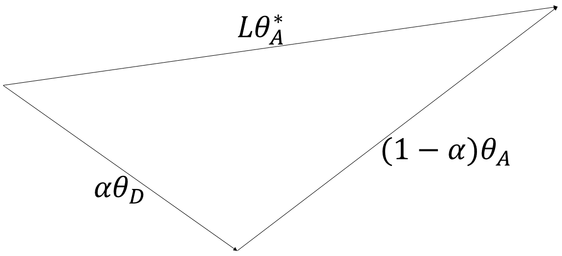
Given that $\lVert\boldsymbol{\theta}_{A}\rVert=\lVert\boldsymbol{\theta}^{*}_{A}\rVert=\lVert\boldsymbol{\theta}_{D}\rVert=1$ , after applying the Law of Cosines to equation 5, we obtain:

(1-\alpha)^{2}=L^{2}+\alpha^{2}-2\alpha L(\boldsymbol{\theta}_{D}\cdot\boldsymbol{\theta}^{*}_{A}),

(6)

where $(\boldsymbol{\theta}_{D}\cdot\boldsymbol{\theta}^{*}_{A})$ has been substituted for $\cos{\measuredangle\left(\boldsymbol{\theta}_{D},\boldsymbol{\theta}^{*}_{A}\right)}$ . Solving the above quadratic equation for $L$ , we obtain:

L=\alpha(\boldsymbol{\theta}_{D}\cdot\boldsymbol{\theta}^{*}_{A})\pm\sqrt{\alpha^{2}(\boldsymbol{\theta}_{D}\cdot\boldsymbol{\theta}^{*}_{A})^{2}-2\alpha+1}.

Note that $1-2\alpha>0$ , $\alpha(\boldsymbol{\theta}_{D}\cdot\boldsymbol{\theta}^{*}_{A})<\sqrt{\alpha^{2}(\boldsymbol{\theta}_{D}\cdot\boldsymbol{\theta}^{*}_{A})^{2}-2\alpha+1}$ . Therefore $\alpha(\boldsymbol{\theta}_{D}\cdot\boldsymbol{\theta}^{*}_{A})-\sqrt{\alpha^{2}(\boldsymbol{\theta}_{D}\cdot\boldsymbol{\theta}^{*}_{A})^{2}-2\alpha+1}<0$ . This would be a contradiction with the fact that $L$ is positive. So it must be the case that:

L=\alpha(\boldsymbol{\theta}_{D}\cdot\boldsymbol{\theta}^{*}_{A})+\sqrt{\alpha^{2}(\boldsymbol{\theta}_{D}\cdot\boldsymbol{\theta}^{*}_{A})^{2}-2\alpha+1}.

Lastly, substituting $L$ in Equation 5 with the right hand side of the above equation results in

\boldsymbol{\theta}_{A}=\frac{\bigg{[}\alpha(\boldsymbol{\theta}_{D}\cdot\boldsymbol{\theta}^{*}_{A})+\sqrt{\alpha^{2}(\boldsymbol{\theta}_{D}\cdot\boldsymbol{\theta}^{*}_{A})^{2}-2\alpha+1}\bigg{]}\boldsymbol{\theta}^{*}_{A}-\alpha\boldsymbol{\theta}_{D}}{(1-\alpha)}.

∎

Appendix E Full Proof of Lemma 2

Proof.

As in Appendix D, consider the vector sum $\alpha\boldsymbol{\theta}_{D}+(1-\alpha)\boldsymbol{\theta}_{A}=L\boldsymbol{\theta}_{C}$ , where $L=\lVert\alpha\boldsymbol{\theta}_{D}+(1-\alpha)\boldsymbol{\theta}_{A}\rVert$ . We consider the general case where $\boldsymbol{\theta}_{C}$ does not necessarily equal $\boldsymbol{\theta}^{*}_{A}$ . Figure 6 shows an illustration of this sum.

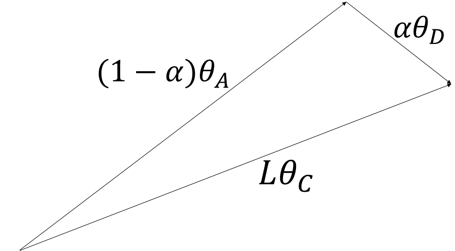
According to the Law of Sines, the following must be true:

\frac{\alpha}{\sin{(\measuredangle\left(\boldsymbol{\theta}_{C},\boldsymbol{\theta}_{A}\right)})}=\frac{1-\alpha}{\sin{(\measuredangle\left(\boldsymbol{\theta}_{C},\boldsymbol{\theta}_{D}\right)})}.

Therefore,

\measuredangle\left(\boldsymbol{\theta}_{C},\boldsymbol{\theta}_{A}\right)=\sin^{-1}{\left(\frac{\alpha\sin{(\measuredangle\left(\boldsymbol{\theta}_{C},\boldsymbol{\theta}_{D}\right)})}{1-\alpha}\right)}.

Now, three cases are possible: (i) $0\leq\measuredangle\left(\boldsymbol{\theta}_{C},\boldsymbol{\theta}_{D}\right)<\frac{\pi}{2}$ , (ii) $\measuredangle\left(\boldsymbol{\theta}_{C},\boldsymbol{\theta}_{D}\right)=\frac{\pi}{2}$ , and (iii) $\frac{\pi}{2}<\measuredangle\left(\boldsymbol{\theta}_{C},\boldsymbol{\theta}_{D}\right)\leq\pi$ . A visualization of each of these cases is shown in Figure 7.

Note that in cases (i) and (iii), $\measuredangle\left(\boldsymbol{\theta}_{C},\boldsymbol{\theta}_{A}\right)=\sin^{-1}{\left(\frac{\alpha\sin{(\measuredangle\left(\boldsymbol{\theta}_{C},\boldsymbol{\theta}_{D}\right))}}{1-\alpha}\right)}<\sin^{-1}{\left(\frac{\alpha}{1-\alpha}\right)}$ because $\left(\frac{\alpha\sin{(\measuredangle\left(\boldsymbol{\theta}_{C},\boldsymbol{\theta}_{D}\right))}}{1-\alpha}\right)<\left(\frac{\alpha}{1-\alpha}\right)$ and because $\sin^{-1}(.)$ is a monotonic function in $[-1,1]$ .

In case (ii), $\measuredangle\left(\boldsymbol{\theta}_{C},\boldsymbol{\theta}_{A}\right)=\sin^{-1}{\left(\frac{\alpha\sin{(\measuredangle\left(\boldsymbol{\theta}_{C},\boldsymbol{\theta}_{D}\right))}}{1-\alpha}\right)}=\sin^{-1}{\left(\frac{\alpha}{1-\alpha}\right)}$ . Therefore, in all cases, $\measuredangle\left(\boldsymbol{\theta}_{C},\boldsymbol{\theta}_{A}\right)\leq\sin^{-1}{\left(\frac{\alpha}{1-\alpha}\right)}$ . Equality is obtained if and only if $\boldsymbol{\theta}_{D}\perp\boldsymbol{\theta}_{C}$ .

∎

Appendix F Additional Lemma Proofs

F.1 Proof of Lemma 3

Proof.

Suppose, by contradiction, there exists a pure strategy Nash equilibrium $(\boldsymbol{\theta}^{\prime}_{D},\boldsymbol{\theta}^{\prime}_{A})$ for $G$ , and $\boldsymbol{\theta}_{C}\neq\boldsymbol{\theta}^{*}_{A}$ . By Lemma 1, there must exist a $\boldsymbol{\theta}_{A}$ given the minority group’s best response $\boldsymbol{\theta}^{\prime}_{D}$ such that $\boldsymbol{\theta}_{C}=\boldsymbol{\theta}_{A}^{*}$ . Note that such a $\boldsymbol{\theta}_{A}$ maximizes the majority group’s utility. Therefore, $\boldsymbol{\theta}_{A}$ produces a better outcome for the majority group than $\boldsymbol{\theta}^{\prime}_{A}$ . However, this raises a contradiction because if $(\boldsymbol{\theta}^{\prime}_{D},\boldsymbol{\theta}^{\prime}_{A})$ is a pure strategy Nash equilibrium, $\boldsymbol{\theta}^{\prime}_{A}$ must be a best response, but $\boldsymbol{\theta}_{A}$ is a better response. Thus, for every pure strategy Nash equilibrium $(\boldsymbol{\theta}^{\prime}_{D},\boldsymbol{\theta}^{\prime}_{A})$ , $\boldsymbol{\theta}_{C}=\boldsymbol{\theta}^{*}_{A}$ .

∎

F.2 Proof of Lemma 4

Proof.

According to Lemma 2, the minority group can pull the aggregate away from $\boldsymbol{\theta}_{A}$ by $\sin^{-1}{\left(\frac{\alpha}{1-\alpha}\right)}$ . In this case, we have $\measuredangle\left(\boldsymbol{\theta}_{C},\boldsymbol{\theta}^{*}_{D}\right)=\left(\boldsymbol{\theta}_{A},\boldsymbol{\theta}^{*}_{D}\right)-\sin^{-1}\left(\frac{\alpha}{1-\alpha}\right)$ . By definition, the largest possible value for $\measuredangle\left(\boldsymbol{\theta}_{A},\boldsymbol{\theta}^{*}_{D}\right)$ is $\pi$ . Therefore, we have

\measuredangle\left(\boldsymbol{\theta}_{C},\boldsymbol{\theta}^{*}_{D}\right)\leq\pi-\sin^{-1}\left(\frac{\alpha}{1-\alpha}\right).

∎

F.3 Proof of Lemma 5

Proof.

Suppose, by contradiction, there is a pure strategy Nash equilibrium where the minority group’s best response $\boldsymbol{\theta}^{\prime}_{D}$ is not orthogonal to $\boldsymbol{\theta}_{C}$ . Consider the majority group’s best response $\boldsymbol{\theta}^{\prime}_{A}$ . By Lemma 2, the most the minority can move the aggregate from $\boldsymbol{\theta}^{\prime}_{A}$ is by $\sin^{-1}\left(\frac{\alpha}{1-\alpha}\right)$ . Therefore, it is possible to obtain any aggregate vector in the cone centered at $\boldsymbol{\theta}^{\prime}_{A}$ with apex angle $2\sin^{-1}\left(\frac{\alpha}{1-\alpha}\right)$ , including the vectors located on its borders. Note that according to Lemma 2, it is only possible to obtain the aggregate vectors on the borders of this cone if $\boldsymbol{\theta}^{\prime}_{D}\perp\boldsymbol{\theta}_{C}$ . Depending on the location of $\boldsymbol{\theta}^{*}_{D}$ relative to this cone, there are three cases:

1.

$\boldsymbol{\theta}^{*}_{D}$ is strictly inside of this cone;
2.

$\boldsymbol{\theta}^{*}_{D}$ is on a border of this cone;
3.

$\boldsymbol{\theta}^{*}_{D}$ is outside of this cone.

See Figure 8 for a visualization of each of these cases.

In all cases that follow, $\boldsymbol{\theta}_{C}=\boldsymbol{\theta}^{*}_{A}$ in this pure strategy Nash equilibrium according to Lemma 3. Additionally, note that if $\boldsymbol{\theta}_{C}$ were on a border of this cone, $\boldsymbol{\theta}^{\prime}_{D}$ would be orthogonal to $\boldsymbol{\theta}_{C}$ according to Lemma 2. However, this would be a contradiction with the given assumption. Therefore, $\boldsymbol{\theta}_{C}=\boldsymbol{\theta}^{*}_{A}$ is strictly inside of this cone.

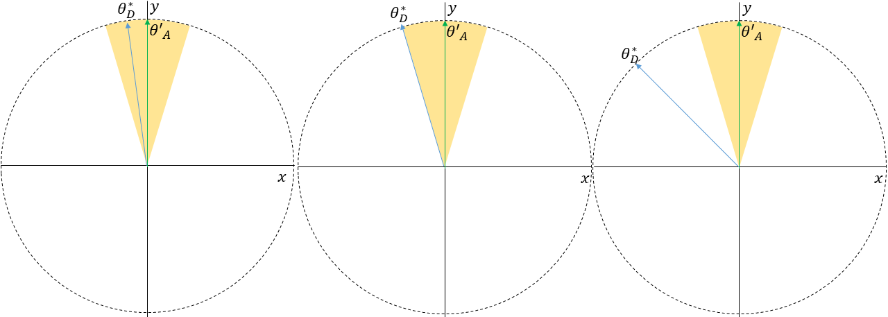
First, consider the case in which $\boldsymbol{\theta}^{*}_{D}$ is strictly inside of this cone. This means that $\exists\boldsymbol{\theta}_{D}:\boldsymbol{\hat{\theta}}_{C}=\frac{(1-\alpha)\boldsymbol{\theta}^{\prime}_{A}+\alpha\boldsymbol{\theta}_{D}}{\lVert(1-\alpha)\boldsymbol{\theta}^{\prime}_{A}+\alpha\boldsymbol{\theta}_{D}\rVert}=\boldsymbol{\theta}^{*}_{D}$ , where $\boldsymbol{\hat{\theta}}_{C}$ is the aggregate obtained from $\boldsymbol{\theta}_{D}$ and $\boldsymbol{\theta}^{\prime}_{A}$ . As mentioned in Section 3 we also assume that $\boldsymbol{\theta}^{*}_{A}\neq\boldsymbol{\theta}^{*}_{D}$ . Therefore, such a $\boldsymbol{\theta}_{D}$ would be a better response than $\boldsymbol{\theta}^{\prime}_{D}$ . However, this raises a contradiction because $\boldsymbol{\theta}^{\prime}_{D}$ is supposed to be a best response, but reporting $\boldsymbol{\theta}_{D}$ such that $\boldsymbol{\hat{\theta}}_{C}=\boldsymbol{\theta}^{*}_{D}$ would be a better response. This means that such a pure strategy Nash equilibrium cannot exist in this case.

Second, consider the case in which $\boldsymbol{\theta}^{*}_{D}$ is on a border of this cone. In this case, $\exists\boldsymbol{\theta}_{D}:\boldsymbol{\theta}_{D}\perp\boldsymbol{\hat{\theta}}_{C};\boldsymbol{\hat{\theta}}_{C}=\frac{(1-\alpha)\boldsymbol{\theta}^{\prime}_{A}+\alpha\boldsymbol{\theta}_{D}}{\lVert(1-\alpha)\boldsymbol{\theta}^{\prime}_{A}+\alpha\boldsymbol{\theta}_{D}\rVert}=\boldsymbol{\theta}^{*}_{D}$ , where $\boldsymbol{\hat{\theta}}_{C}$ is the aggregate obtained from $\boldsymbol{\theta}_{D}$ and $\boldsymbol{\theta}^{\prime}_{A}$ . This also raises a contradiction because there exists a better response than $\boldsymbol{\theta}^{\prime}_{D}$ (that obtains $\boldsymbol{\hat{\theta}}_{C}=\boldsymbol{\theta}^{*}_{D}$ ) for the minority group that is orthogonal to the aggregate vector $\boldsymbol{\hat{\theta}}_{C}$ that results. In turn, such a pure strategy Nash equilibrium cannot exist in this case either.

Lastly, consider the case in which $\boldsymbol{\theta}^{*}_{D}$ is outside of this cone. In this case, $\exists\boldsymbol{\theta}_{D}:\boldsymbol{\theta}_{D}\perp\boldsymbol{\hat{\theta}}_{C};\boldsymbol{\hat{\theta}}_{C}=\frac{(1-\alpha)\boldsymbol{\theta}^{\prime}_{A}+\alpha\boldsymbol{\theta}_{D}}{\lVert(1-\alpha)\boldsymbol{\theta}^{\prime}_{A}+\alpha\boldsymbol{\theta}_{D}\rVert}$ , where $\boldsymbol{\hat{\theta}}_{C}$ is the aggregate obtained from $\boldsymbol{\theta}_{D}$ and $\boldsymbol{\theta}^{\prime}_{A}$ , and $\boldsymbol{\hat{\theta}}_{C}$ is on a border of the cone. More specifically, there are two such $\boldsymbol{\hat{\theta}}_{C}$ because there are two borders. Recall regarding the original aggregate that $\boldsymbol{\theta}_{C}=\boldsymbol{\theta}^{*}_{A}$ . Moreover, $\boldsymbol{\theta}_{C}=\boldsymbol{\theta}^{*}_{A}$ is strictly inside of this cone. As a result, one of the borders will be closer to $\boldsymbol{\theta}^{*}_{D}$ than $\boldsymbol{\theta}^{*}_{A}$ . Therefore, at least one $\boldsymbol{\hat{\theta}}_{C}$ will satisfy $\boldsymbol{\hat{\theta}}_{C}\cdot\boldsymbol{\theta}^{*}_{D}>\boldsymbol{\theta}^{*}_{A}\cdot\boldsymbol{\theta}^{*}_{D}$ . This raises a contradiction as well because there exists a better response than $\boldsymbol{\theta}^{\prime}_{D}$ for the minority group that is orthogonal to the aggregate vector $\boldsymbol{\hat{\theta}}_{C}$ that results. It is therefore evident that such a pure strategy Nash equilibrium cannot exist in this case as well.

Thus, via proof by contradiction and cases, in any pure strategy Nash equilibrium, the minority group’s best response is orthogonal to $\boldsymbol{\theta}_{C}$ . Moreover, in order to obtain $\boldsymbol{\theta}_{C}=\boldsymbol{\theta}^{*}_{A}$ according to Lemma 3 with $\boldsymbol{\theta}^{\prime}_{D}\perp\boldsymbol{\theta}_{C}$ , $\boldsymbol{\theta}^{\prime}_{A}$ will offset their response from their true preferences $\boldsymbol{\theta}^{*}_{A}$ by $\sin^{-1}\left(\frac{\alpha}{1-\alpha}\right)$ . ∎

Appendix G Algebraic Simplification for Proof of Theorem 2

Equation 2 is given by

\boldsymbol{\theta}_{A}=\frac{\bigg{[}\alpha(\boldsymbol{\theta}_{D}\cdot\boldsymbol{\theta}^{*}_{A})+\sqrt{\alpha^{2}(\boldsymbol{\theta}_{D}\cdot\boldsymbol{\theta}^{*}_{A})^{2}-2\alpha+1}\bigg{]}\boldsymbol{\theta}^{*}_{A}-\alpha\boldsymbol{\theta}_{D}}{(1-\alpha)}.

Whenever $\boldsymbol{\theta}_{D}\perp\boldsymbol{\theta}_{C}$ ,

	$\displaystyle\alpha(\boldsymbol{\theta}_{D}\cdot\boldsymbol{\theta}^{}_{A})+\sqrt{\alpha^{2}(\boldsymbol{\theta}_{D}\cdot\boldsymbol{\theta}^{}_{A})^{2}-2\alpha+1}$	$\displaystyle=\lVert\alpha\boldsymbol{\theta}_{D}+(1-\alpha)\boldsymbol{\theta}_{A}\rVert$
		$\displaystyle=\sqrt{(1-\alpha)^{2}-\alpha^{2}}$
		$\displaystyle=\sqrt{1-2\alpha}.$

$\boldsymbol{\theta}_{D}\perp\boldsymbol{\theta}_{C}$ in this case because $\boldsymbol{\theta}_{D}=\boldsymbol{\theta}^{\prime}_{D}=\mathrm{sign}(\boldsymbol{\theta}^{*}_{D}\cdot R\boldsymbol{\theta}^{*}_{A})R\boldsymbol{\theta}^{*}_{A}$ and $\boldsymbol{\theta}^{*}_{A}=\boldsymbol{\theta}_{C}$ . Substitution of values into Equation 2 yields

	$\displaystyle\boldsymbol{\theta}^{\prime}_{A}$	$\displaystyle=\frac{\left(\sqrt{1-2\alpha}\right)\boldsymbol{\theta}^{}_{A}-\alpha\mathrm{sign}(\boldsymbol{\theta}^{}_{D}\cdot R\boldsymbol{\theta}^{}_{A})R\boldsymbol{\theta}^{}_{A}}{(1-\alpha)},$
		$\displaystyle=\frac{\big{[}(\sqrt{1-2\alpha})I-\alpha\mathrm{sign}(\boldsymbol{\theta}^{}_{D}\cdot R\boldsymbol{\theta}^{}_{A})R\big{]}\boldsymbol{\theta}^{*}_{A}}{1-\alpha}.$

	$\displaystyle\measuredangle\left(\boldsymbol{\theta}^{\prime}_{A},\boldsymbol{\theta}^{}_{A}\right)+\measuredangle\left(\boldsymbol{\theta}^{}_{A},\boldsymbol{\theta}^{*}_{D}\right)$	$\displaystyle>\measuredangle\left(\boldsymbol{\theta}^{\prime}_{A},\boldsymbol{\theta}^{*}_{D}\right),$
	$\displaystyle\measuredangle\left(\boldsymbol{\theta}^{}_{A},\boldsymbol{\theta}^{}_{D}\right)$	$\displaystyle>\measuredangle\left(\boldsymbol{\theta}^{\prime}_{A},\boldsymbol{\theta}^{}_{D}\right)-\measuredangle\left(\boldsymbol{\theta}^{\prime}_{A},\boldsymbol{\theta}^{}_{A}\right).$