MonoNeRF: Learning a Generalizable Dynamic Radiance Field
from Monocular Videos

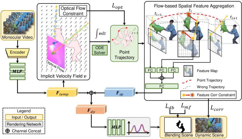
MonoNeRF aims to model generalizable radiance field of dynamic scenes. Our method takes multiple monocular videos as input and uses optical flows, depth maps, and binary masks of foreground objects as supervision signals. Those signals could be generated by pretrained models automatically. We build the generalizable static and dynamic fields for backgrounds and foregrounds separately. For generalizable dynamic field, we suppose that spatio-temporal points flow along their trajectories and hold consistent features over time. We first extract video features by a CNN encoder and generate the temporal feature vectors based on the extracted features. Then, we build an implicit velocity field from the temporal feature vectors to estimate point trajectories. Next, we exploit the estimated point trajectories as indexes to find the local image patches on each frame and extract the spatial features from the patches with the proposed flow-based feature aggregation module. Different from NeRF [28] that uses scene-agnostic point positions to render image color, we aggregate the scene-dependent spatial and temporal features as the final point features to render foreground scenes with volume rendering. Finally, we design the optical flow and feature correspondence constraints for jointly learning point features and trajectories. For generalizable static field, we suppose backgrounds are static and each video frame is considered as a different view of the background. Since some background parts may be occluded by the foreground, we design an effective strategy to sample background point features. In the end, we combine the generalizable static and dynamic fields for rendering free-point videos.

In this section, we introduce our generalizable dynamic field that renders novel views of dynamic foregrounds. We denote a monocular video as $\boldsymbol{V}=\{\boldsymbol{V}^{i},i=1,2...,K\}$ consisting of $K$ frames . For each frame $\boldsymbol{V}^{i}$, $t_{i}$ is the observed timestamp and $\Pi^{i}$ is the projection transform from the world coordinate to the 2D frame pixel coordinate. As Figure 2 shows, given a video $\boldsymbol{V}$, we exploit a video encoder $E_{dy}$ to extract the video feature vector represented as $E_{dy}(\boldsymbol{V})$ and generate the temporal feature vector $\boldsymbol{F}_{temp}$ with a multiple layer perceptron (MLP) $W_{temp}$: $E_{dy}(\boldsymbol{V})\rightarrow\boldsymbol{F}_{temp}$. We build the implicit velocity field based on $\boldsymbol{F}_{temp}$.

Implicit velocity field. We suppose points are moving in the scene and represent a spatio-temporal point as $\boldsymbol{p}=(\boldsymbol{x}_{p},t_{p})$ including the 3D point position $\boldsymbol{x}_{p}$ and time $t_{p}$. We define $\boldsymbol{\Phi}$ as the continuous point trajectory and $\boldsymbol{\Phi}(\boldsymbol{p},t)$ denotes the position of point $\boldsymbol{p}$ at timestamp $t$. We further define the velocity field $\boldsymbol{v}$ which includes the 3D velocity of each point. The relationship between point velocity and trajectory is specified as follows,

$$\frac{\partial\boldsymbol{\Phi}(\boldsymbol{p},t)}{\partial t}=\boldsymbol{v}\Big{(}\boldsymbol{\Phi}(\boldsymbol{p},t),t\Big{)},\ \ \text{ s.t. }\boldsymbol{\Phi}(\boldsymbol{p},t_{p})=\boldsymbol{x}_{p}.$$

(1)

$\boldsymbol{v}$ is conditioned on $\boldsymbol{F}_{temp}$ and implemented by an MLP $W_{vel}$: $(\boldsymbol{F}_{temp}(\boldsymbol{V}),\boldsymbol{\Phi},t)\rightarrow\boldsymbol{v}$. We calculate the point trajectory at an observed timestamp $t_{i}$ with Neural ODE [5],

$$\boldsymbol{\Phi}(\boldsymbol{p},t_{i})=\boldsymbol{x}_{p}+\int_{t_{p}}^{t_{i}}\boldsymbol{v}\big{(}\boldsymbol{\Phi}(\boldsymbol{p},t),t\big{)}dt.$$

(2)

We take $\boldsymbol{\Phi}(\boldsymbol{p},t_{i})$ as an index to query the spatial feature.

Flow-based spatial feature aggregation. We employ $\Pi^{i}$ to project $\boldsymbol{\Phi}(\boldsymbol{p},t_{i})$ on $\boldsymbol{V}^{i}$ and find the local image patch indexed by the projected position $\Pi^{i}(\boldsymbol{\Phi}(\boldsymbol{p},t_{i}))$. We extract the feature vector $\boldsymbol{F}_{sp}^{i}$ from the patch with the encoder $E_{dy}$ and a fully connected layer $fc_{1}$,

$$\boldsymbol{F}_{sp}^{i}(\boldsymbol{V};\boldsymbol{p})=fc_{1}\Big{(}E_{dy}\big{(}\boldsymbol{V}^{i};\Pi^{i}(\boldsymbol{\Phi}(\boldsymbol{p},t_{i}))\big{)}\Big{)}.$$

(3)

In practice, $E_{dy}\big{(}\boldsymbol{V}^{i};\Pi^{i}(\boldsymbol{\Phi}(\boldsymbol{p},t_{i}))\big{)}$ is implemented by using $E_{dy}$ to extract the frame-wise feature map of $\boldsymbol{V}^{i}$ and sampling the feature vector at $\Pi^{i}(\boldsymbol{\Phi}(\boldsymbol{p},t_{i}))$ with bilinear interpolation. The spatial feature vector $\boldsymbol{F}_{sp}$ is then calculated by incorporating $\{\boldsymbol{F}_{sp}^{1},\boldsymbol{F}_{sp}^{2},...,\boldsymbol{F}_{sp}^{K}\}$ with a fully connected layer $fc_{2}$,

$$\boldsymbol{F}_{sp}(\boldsymbol{V};\boldsymbol{p})=fc_{2}\big{(}\boldsymbol{F}_{sp}^{1}(\boldsymbol{V};\boldsymbol{p}),\boldsymbol{F}_{sp}^{2}(\boldsymbol{V};\boldsymbol{p}),...,\boldsymbol{F}_{sp}^{K}(\boldsymbol{V};\boldsymbol{p})\big{)}.$$

(4)

Finally, we incorporate $\boldsymbol{F}_{temp}$ and $\boldsymbol{F}_{sp}$ as the point feature vector $\boldsymbol{F}_{dy}$,

$$\boldsymbol{F}_{dy}(\boldsymbol{V};\boldsymbol{p})=concat\{\boldsymbol{F}_{temp}(\boldsymbol{V}),\boldsymbol{F}_{sp}(\boldsymbol{V};\boldsymbol{p})\}.$$

(5)

We build the generalizable dynamic field based on $\boldsymbol{F}_{dy}$.

Dynamic foreground rendering. Taking a point $\boldsymbol{p}$ and its feature vector $\boldsymbol{F}_{dy}(\boldsymbol{V};\boldsymbol{p})$ as input, our generalizable dynamic radiance field $W_{dy}$: $(\boldsymbol{p},\boldsymbol{F}_{dy}(\boldsymbol{V};\boldsymbol{p}))\rightarrow(\boldsymbol{c}_{dy},\sigma_{dy},b)$ predicts the volume density $\sigma_{dy}$, color $\boldsymbol{c}_{dy}$ and blending weight $b$ of the point. We follow DynNeRF [13] and utilize $b$ to judge whether a point belongs to static background or dynamic foreground. We exploit volume rendering to approximate each pixel color of an image. Concretely, given a ray $\boldsymbol{r}(u)=\boldsymbol{o}+u\boldsymbol{d}$ starting from the camera center $\boldsymbol{o}$ along the direction $\boldsymbol{d}$ through a pixel, its color is integrated by

$$\boldsymbol{C}_{dy}(\boldsymbol{r})=\int_{u_{n}}^{u_{f}}T_{dy}(u)\sigma_{dy}(u)\boldsymbol{c}_{dy}(u)du,$$

(6)

where $u_{n},u_{f}$ are the bounds of the volume rendering depth range and $T_{dy}(u)=exp(-\int_{u_{n}}^{u}\sigma_{dy}(\boldsymbol{r}(s))ds$ is the accumulated transparency. We simplify $\boldsymbol{c}(u)=\boldsymbol{c}(\boldsymbol{r}(u),\boldsymbol{d})$ and $\sigma(u)=\sigma(\boldsymbol{r}(u))$ here and in the following sections. Next we present the optical flow and feature correspondence constraints that jointly supervise our model.

Optical flow constraint. We supervise $\boldsymbol{v}$ with the optical flow $\boldsymbol{f}^{gt}$. In practice, it can only approximate the backward flow $\boldsymbol{f}_{bw}^{gt}$ and forward flow $\boldsymbol{f}_{fw}^{gt}$ between two consecutive video frames [40]. We hence estimate the point backward and forward trajectory variations during the period that the point passes between two frames and calculate optical flows by integrating the trajectory variations of each point along camera rays. Formally, given a ray $\boldsymbol{r}(u)$ through a pixel on the frame $\boldsymbol{V}^{i}$ at time $t_{i}$, for each point on the ray i.e., $\boldsymbol{p}(u)=(\boldsymbol{r}(u),t_{i})$ the trajectory variations $\Delta\boldsymbol{\Phi}_{bw}$ back to $t_{i-1}$ and $\Delta\boldsymbol{\Phi}_{fw}$ forward to $t_{i+1}$ are obtained by the following equation,

$$\Delta\boldsymbol{\Phi}_{\{bw,fw\}}(\boldsymbol{p}(u))=\int_{t_{i}}^{t_{\{i-1,i+1\}}}\boldsymbol{v}\Big{(}\boldsymbol{\Phi}(\boldsymbol{p}(u),t),t\Big{)}dt.$$

(7)

We follow previous works [21, 13] and exploit the volume rendering to integrate pseudo optical flows $\boldsymbol{f}_{bw}$ and $\boldsymbol{f}_{fw}$ by utilizing the estimated volume density $\sigma_{dy}$ of each point,

$$\boldsymbol{f}_{\{bw,fw\}}(\boldsymbol{r})=\int_{u_{n}}^{u_{f}}T_{dy}(u)\sigma_{dy}(u)\Delta\boldsymbol{\Phi}_{\{bw,fw\}}^{i}(\boldsymbol{p}(u))du,$$

(8)

where $\Delta\boldsymbol{\Phi}_{\{bw,fw\}}^{i}=\Pi^{i}(\Delta\boldsymbol{\Phi}_{\{bw,fw\}})$ denotes we use $\Pi^{i}$ to project 3D trajectory variations on the image plane of $\boldsymbol{V}^{i}$. We supervise the pseudo flows by the ground truth flows,

$$L_{opt}=\sum_{\boldsymbol{r}}\Big{(}\boldsymbol{f}_{\{bw,fw\}}(\boldsymbol{r})-\boldsymbol{f}_{\{bw,fw\}}^{gt}(\boldsymbol{r})\Big{)}.$$

(9)

In this way, the relation of point trajectories along a ray is limited by the optical flow supervision.

Feature correspondence constraint. According to Section 3.1, a point moving along the trajectory holds the same feature and represents the consistent color and density. For each ray $\boldsymbol{r}_{curr}$ at the current time $t_{i}$ through a pixel of $\boldsymbol{V}^{i}$, we warp the ray from the neighboring observed timestamps $t_{i-1}$ and $t_{i+1}$ as $\boldsymbol{r}_{bw}$ and $\boldsymbol{r}_{fw}$ separately by using (7),

$$\boldsymbol{r}_{\{bw,fw\}}(u)=\boldsymbol{r}_{curr}(u)+\Delta\boldsymbol{\Phi}_{\{bw,fw\}}(\boldsymbol{p}_{curr}(u)),$$

(10)

where $\boldsymbol{p}_{curr}(u)=(\boldsymbol{r}_{curr}(u),t_{i})$. We render the pixel color from the point features not only along the ray $\boldsymbol{r}_{curr}$ at the time $t_{i}$, but also along the wrapped rays $\boldsymbol{r}_{bw}$ at $t_{i-1}$ and $\boldsymbol{r}_{fw}$ at $t_{i+1}$. The predicted pixel color $\boldsymbol{C}_{dy}$ is rendered by using (6) and supervised by the ground truth colors $\boldsymbol{C}_{dy}^{gt}$,

$$L_{\{bw,curr,fw\}}=\sum_{\boldsymbol{r}}||\boldsymbol{C}_{dy}(\boldsymbol{r}_{\{bw,curr,fw\}})-\boldsymbol{C}_{dy}^{gt}(\boldsymbol{r})||_{2}.$$

(11)

The feature correspondence constraint $L_{corr}$ is defined as

$$L_{corr}=L_{bw}+L_{curr}+L_{fw}.$$

(12)

$L_{corr}$ supervises the predicted color and point features $\boldsymbol{F}_{dy}$.

As mentioned in Section 3.1, for some background parts occluded by the changing foreground in the current view, their features implying the foreground cannot infer the correct background information. However, the occluded parts could be seen in non-occluded views with correct background features. To this end, given a point position $\boldsymbol{x}$, the background point feature vector $\boldsymbol{F}_{st}$ is produced by

$$\boldsymbol{F}_{st}(\boldsymbol{V};\boldsymbol{x})=fc_{3}\Big{(}E_{st}(\boldsymbol{V}^{*};\Pi^{*}(\boldsymbol{x}))\Big{)},$$

(13)

where $fc_{3}$ is a fully connected layer and $E_{st}$ denotes the image encoder. $\boldsymbol{V}^{*}$ and $\Pi^{*}$ are the non-occluded frame and corresponding projection transform respectively. $E_{st}(\boldsymbol{V}^{*};\Pi^{*}(\boldsymbol{x}))$ denotes that we find the local image patch at $\Pi^{*}(\boldsymbol{x})$ and extract the feature vectors with an image encoder $E_{st}$ similar to $E_{dy}\big{(}\boldsymbol{V}^{i};\Pi^{i}(\boldsymbol{\Phi}(\boldsymbol{p},t_{i}))\big{)}$. Since there is no prior in which frames they can be exposed, we apply a straightforward yet effective strategy by randomly sampling one frame from the other frames in the video. We represent the static scene as a radiance field to infer the color $\boldsymbol{c}_{st}$ and density $\sigma_{st}$ by using an MLP $W_{st}$: $(\boldsymbol{x},\boldsymbol{d},\boldsymbol{F}_{st}(\boldsymbol{V};\boldsymbol{x}))\rightarrow(\boldsymbol{c}_{st},\sigma_{st})$. The expected background color $\boldsymbol{C}_{st}$ is given by

$$\boldsymbol{C}_{st}(\boldsymbol{r})=\int_{u_{n}}^{u_{f}}T_{st}(u)\sigma_{st}(u)\boldsymbol{c}_{st}(u)du,$$

(14)

where $T_{st}(t)=exp(-\int_{u_{n}}^{u}\sigma_{st}(\boldsymbol{r}(s))ds$. We employ foreground masks $M$ to optimize the static field by supervising the pixel color in each video frame in the background regions (where $M(\boldsymbol{r})=0$),

$$L_{st}=\sum_{\boldsymbol{r}}||(\boldsymbol{C}_{st}(\boldsymbol{r})-\boldsymbol{C}_{st}^{gt}(\boldsymbol{r}))(1-M(\boldsymbol{r}))||_{2},$$

(15)

where $\boldsymbol{C}_{st}^{gt}$ represents the ground truth color.

The final dynamic scene color combines the colors from the generalizable dynamic and static fields,

$$\begin{split}\boldsymbol{C}_{full}(\boldsymbol{r})=&\int_{u_{n}}^{u_{f}}T_{full}(u)\sigma_{full}(u)\boldsymbol{c}_{full}(u)du,\end{split}$$

(16)

where

$$\sigma_{full}(u)\boldsymbol{c}_{full}(u)=(1-b)\sigma_{st}(u)\boldsymbol{c}_{st}(u)+b\sigma_{dy}(u)\boldsymbol{c}_{dy}(u),$$

(17)

and applies the reconstruction loss,

$$L_{full}=\sum_{\boldsymbol{r}}||\boldsymbol{C}_{full}(\boldsymbol{r})-\boldsymbol{C}_{full}^{gt}(\boldsymbol{r})||_{2}.$$

(18)

Next we design several strategies to optimize our model.

Point trajectory discretization. While point trajectory can be numerically estimated by the continuous integral (2) with Neural ODE solvers [5], it needs plenty of time for querying each point trajectory. To accelerate the process, we propose to partition $[t_{p},t_{i}]$ into $N$ evenly-spaced bins and suppose the point velocity in each bin is a constant. The point trajectory can be estimated by the following equation,

$$\boldsymbol{\Phi}(\boldsymbol{p},t_{i})=\boldsymbol{x}_{p}+\sum_{n=1}^{N}\boldsymbol{v}\big{(}\boldsymbol{\Phi}(\boldsymbol{p},t+\Delta t),t+\Delta t\big{)}\Delta t,$$

(19)

where $\Delta t=\frac{n}{N}(t_{i}-t_{p})$.

Depth-blending restriction. To calculate the blending weights within a foreground ray in the generalizable dynamic field, only the points in close proximity to the estimated ray depth are regarded as foreground points, whereas points beyond this range are excluded. We penalize the blending weights of non-foreground points in foreground rays. Specifically, given a ray $\boldsymbol{r}(u)$ through a pixel and the pixel depth $u_{d}$, We penalize the blending weights of the points on the ray out of the interval $(u_{d}-\epsilon,u_{d}+\epsilon)$,

$$L_{db}=\sum_{u\in(u_{n},u_{d}-\epsilon)\cup(u_{d}+\epsilon,u_{f})}||b(\boldsymbol{r}(u))||_{2},$$

(20)

where $b(\boldsymbol{r}(u))$ is the blending weight at the position $\boldsymbol{r}(u)$. $\epsilon$ controls the surface thickness of the dynamic foreground.

Mask flow loss. We further constrain the consistency of point features by minimizing blending weight variations along trajectories,

$$L_{mf}=\sum_{i,j\in\{1,2,..,K\}}||b(\boldsymbol{\Phi}(\boldsymbol{p},t_{i}))-b(\boldsymbol{\Phi}(\boldsymbol{p},t_{j}))||_{2},$$

(21)

where $b(\boldsymbol{\Phi}(\boldsymbol{p},t))$ denotes the blending weight at $\boldsymbol{\Phi}(\boldsymbol{p},t)$.

Other regularization. We follow previous works [21, 13, 10] to use the depth constraint, sparsity constraint, and motion regularization and smoothness to train the model.

Dataset. We used the Dynamic Scene dataset [54] to evaluate the proposed method. Concretely, it contains 9 video sequences that are captured with 12 cameras by using a camera rig. We followed previous works [21, 13] and derived each frame of the video from different cameras to simulate the camera motion. All the cameras capture images at 12 different timestamps $\{t_{i},i=1,2...,12\}$. Each training video contains twelve frames sampled from the $i^{th}$ camera at time $t_{i}$ followed DynNeRF [13]. We used COLMAP [36, 37] to approximate the camera poses. It is assumed intrinsic parameters of all the cameras are the same. DynamicFace sequences were excluded because COLMAP fails to estimate camera poses. All video frames were resized to 480$\times$270 resolution. We generated the depth, mask, and optical flow signals from the depth estimation model [35], Mask R-CNN [16], and RAFT [40].

Implementation details. We followed pixelNeRF [55] and used ResNet-based MLPs as our implicit velocity field $W_{vel}$ and rendering networks $W_{dy}$ and $W_{st}$. For generalizable dynamic field, we utilized Slowonly50 [11] pretrained on Kinetics400 [2] dataset as the encoder $E_{dy}$ with the frozen weights. We removed the final fully connected layer in the backbone and incorporated the first, second, and third feature layers for querying $\boldsymbol{F}_{sp}$. We simplified (4) that $\boldsymbol{F}_{sp}$ at time $t_{i}$ is sampled from $\{\boldsymbol{V}^{i-1},\boldsymbol{V}^{i},\boldsymbol{V}^{i+1}\}$. For generalizable static field, we used ResNet18 [17] pretrained on ImageNet [8] as the encoder $E_{st}$. We extracted a feature pyramid from video frames for querying $\boldsymbol{F}_{st}$. The vector sizes of $\boldsymbol{F}_{temp}$, $\boldsymbol{F}_{sp}$, $\boldsymbol{F}_{dy}$, and $\boldsymbol{F}_{st}$ are 256. Please refer to the supplementary material for more details.

In this section, we trained the models from single monocular videos, where existing methods are applicable to this setting. Specifically, we first tested the performance on training frames, which is the widely-used setting to evaluate video-based NeRFs. Then, we tested the generalization ability on unseen frames in the video, where other existing methods are not able to transfer well to the unseen motions.

Novel view synthesis on training frames. To evaluate the synthesized novel views, we followed DynNeRF [13] and tested the performance by fixing the view to the first camera and changing time. We reported the PSNR and LPIPS [56] in Table 1. We evaluated the performance of Li et al. [21], Tretschk et al. [41], NeuPhysics [34], and Chen et al. [13] from the official implementations. Even without the need of generalization ability, our method achieves better results.

Novel view synthesis on unseen frames. We split the video frames into two groups: four front frames were used for training and the rest of eight unseen frames were utilized to render novel views. Figure 4 shows that our model successfully renders new motions in the unseen frames, while DynNeRF [13] only interpolates novel views in the training frames. The reported PSNR, SSIM [48], and LPIPS scores in Table 2 quantitatively verify the superiority of our model.

In the section, we tested the novel view synthesis performance on multiple dynamic scenes. It is worth noting that as existing methods can only learn from single monocular videos, they are not applicable to the settings that need to train on multiple videos. Then, we evaluated the novel scene adaption ability on several novel monocular videos. Lastly, we conducted a series of scene editing experiments.

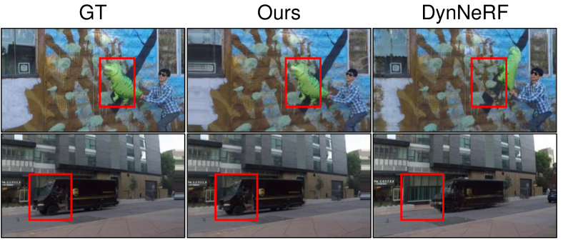
Novel view synthesis on training videos. We selected Balloon2 and Umbrella scenes to train our model. As shown in Figure 3 and Table 3, our model could distinguish foregrounds from two scenes and perform well with $\boldsymbol{F}_{dy}$. Specifically, it predicts generalizable scene flows with $\boldsymbol{F}_{temp}$ and renders more accurate details with $\boldsymbol{F}_{sp}$.

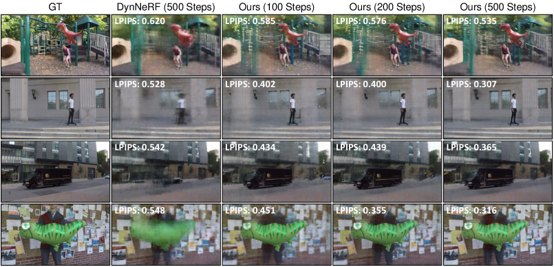
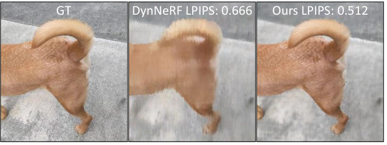
Novel view synthesis on unseen videos. We explored the generalization ability of our model by pretraining on the Balloon2 scene and fine-tuning the pretrained model on other scenes. Figure 5 presents the results of four unseen videos: Playground, Skating, Truck, and Balloon1. We also pretrained DynNeRF [13] on the Balloon2 scene for a fair comparison. While DynNeRF only learns to render new scenes from scratch, our model transfers to scenes with correct dynamic motions. By further training with 500 steps, our model achieves better image rendering quality and higher LPIPS scores, which takes about 10 minutes.

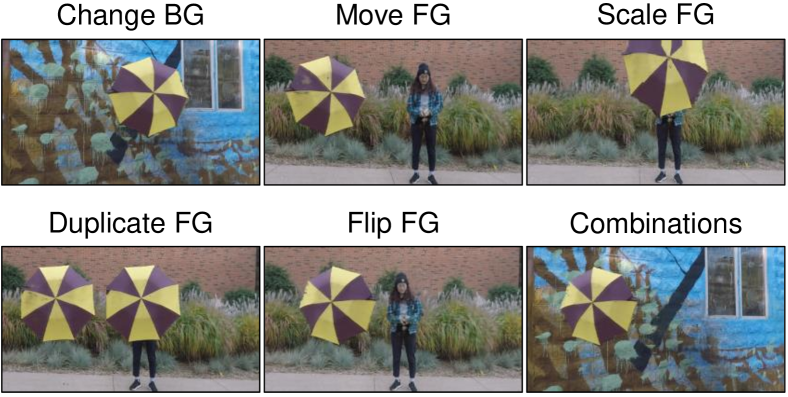
Scene editing. As Figure 6 shows, our model further supports many scene editing applications by directly processing point features without extra training. Changing background was implemented by exchanging the static scene features between two scenes. Moving, scaling, duplicating and flipping foreground were directly applied by operating video features in dynamic radiance field. The above applications could be combined arbitrarily.

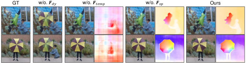
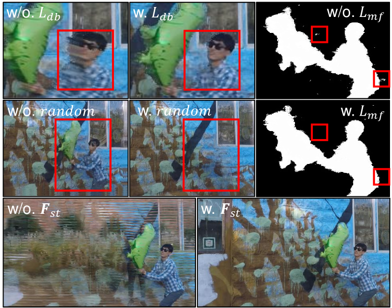
We conducted a series of experiments to examine the proposed $L_{db}$, $L_{mf}$, $\boldsymbol{F}_{st}$, random sampling strategy, and trajectory discretization method. We show in Figure 7 that $L_{db}$ deblurs the margin of the synthesized foreground in novel views, $L_{mf}$ keeps the blending consistency in different views for delineating the foreground more accurately, The random sampling strategy successfully renders static scene without dynamic foreground, and backgrounds of two scenes are mixed without $\boldsymbol{F}_{st}$. We also show the numeric comparisons of $L_{db},L_{mf},\boldsymbol{F}_{st}$, and random sampling strategy in Table 4. In Table 5, our discretization method reaches comparable results with ODE solvers [5] and achieves higher performance with the increase of $N$.

References

- [1] Shengqu Cai, Anton Obukhov, Dengxin Dai, and Luc Van Gool. Pix2NeRF: Unsupervised conditional -GAN for single image to neural radiance fields translation. In CVPR, pages 3971–3980, 2022.
- [2] Joao Carreira and Andrew Zisserman. Quo vadis, action recognition? a new model and the kinetics dataset. In CVPR, pages 6299–6308, 2017.
- [3] Eric Chan, Marco Monteiro, Petr Kellnhofer, Jiajun Wu, and Gordon Wetzstein. pi-GAN: Periodic implicit generative adversarial networks for 3D-aware image synthesis. In CVPR, 2021.
- [4] Anpei Chen, Zexiang Xu, Fuqiang Zhao, Xiaoshuai Zhang, Fanbo Xiang, Jingyi Yu, and Hao Su. MVSNeRF: Fast generalizable radiance field reconstruction from multi-view stereo. In ICCV, pages 14124–14133, 2021.
- [5] Ricky T. Q. Chen, Yulia Rubanova, Jesse Bettencourt, and David K Duvenaud. Neural ordinary differential equations. In S. Bengio, H. Wallach, H. Larochelle, K. Grauman, N. Cesa-Bianchi, and R. Garnett, editors, NeurIPS, volume 31, 2018.
- [6] Shenchang Eric Chen and Lance Williams. View interpolation for image synthesis. In Proceedings of the 20th annual conference on Computer graphics and interactive techniques, pages 279–288, 1993.
- [7] Xingyu Chen, Qi Zhang, Xiaoyu Li, Yue Chen, Ying Feng, Xuan Wang, and Jue Wang. Hallucinated neural radiance fields in the wild. In CVPR, pages 12943–12952, 2022.
- [8] Jia Deng, Wei Dong, Richard Socher, Li-Jia Li, Kai Li, and Li Fei-Fei. ImageNet: A large-scale hierarchical image database. In CVPR, pages 248–255, 2009.
- [9] Kangle Deng, Andrew Liu, Jun-Yan Zhu, and Deva Ramanan. Depth-supervised NeRF: Fewer views and faster training for free. In CVPR, June 2022.
- [10] Yilun Du, Yinan Zhang, Hong-Xing Yu, Joshua B. Tenenbaum, and Jiajun Wu. Neural radiance flow for 4d view synthesis and video processing. In ICCV, 2021.
- [11] Christoph Feichtenhofer, Haoqi Fan, Jitendra Malik, and Kaiming He. SlowFast networks for video recognition. In ICCV, pages 6201–6210, 2019.
- [12] Guy Gafni, Justus Thies, Michael Zollhöfer, and Matthias Nießner. Dynamic neural radiance fields for monocular 4d facial avatar reconstruction. In CVPR, pages 8649–8658, June 2021.
- [13] Chen Gao, Ayush Saraf, Johannes Kopf, and Jia-Bin Huang. Dynamic view synthesis from dynamic monocular video. In ICCV, 2021.
- [14] Steven J Gortler, Radek Grzeszczuk, Richard Szeliski, and Michael F Cohen. The lumigraph. In ACM SIGGRAPH, pages 43–54, 1996.
- [15] Jiatao Gu, Lingjie Liu, Peng Wang, and Christian Theobalt. StyleNeRF: A style-based 3D aware generator for high-resolution image synthesis. In ICLR, 2022.
- [16] Kaiming He, Georgia Gkioxari, Piotr Dollar, and Ross Girshick. Mask r-cnn. In ICCV, Oct 2017.
- [17] Kaiming He, X. Zhang, Shaoqing Ren, and Jian Sun. Deep residual learning for image recognition. CVPR, pages 770–778, 2016.
- [18] Wonbong Jang and Lourdes Agapito. CodeNeRF: Disentangled neural radiance fields for object categories. In ICCV, pages 12949–12958, October 2021.
- [19] Marc Levoy and Pat Hanrahan. Light field rendering. In ACM SIGGRAPH, 1996.
- [20] Tianye Li, Mira Slavcheva, Michael Zollhöfer, Simon Green, Christoph Lassner, Changil Kim, Tanner Schmidt, Steven Lovegrove, Michael Goesele, Richard Newcombe, and Zhaoyang Lv. Neural 3D video synthesis from multi-view video. In CVPR, pages 5521–5531, June 2022.
- [21] Zhengqi Li, Simon Niklaus, Noah Snavely, and Oliver Wang. Neural scene flow fields for space-time view synthesis of dynamic scenes. In CVPR, 2021.
- [22] Lingjie Liu, Jiatao Gu, Kyaw Zaw Lin, Tat-Seng Chua, and Christian Theobalt. Neural sparse voxel fields. In NeurIPS, volume 33, 2020.
- [23] Lingjie Liu, Marc Habermann, Viktor Rudnev, Kripasindhu Sarkar, Jiatao Gu, and Christian Theobalt. Neural actor: Neural free-view synthesis of human actors with pose control. ACM Trans. Graph.(ACM SIGGRAPH Asia), 2021.
- [24] Xingyu Liu, Charles R Qi, and Leonidas J Guibas. Flownet3D: Learning scene flow in 3D point clouds. In CVPR, pages 529–537, 2019.
- [25] Yuan Liu, Sida Peng, Lingjie Liu, Qianqian Wang, Peng Wang, Theobalt Christian, Xiaowei Zhou, and Wenping Wang. Neural rays for occlusion-aware image-based rendering. In CVPR, 2022.
- [26] Ricardo Martin-Brualla, Noha Radwan, Mehdi S. M. Sajjadi, Jonathan T. Barron, Alexey Dosovitskiy, and Daniel Duckworth. NeRF in the Wild: Neural radiance fields for unconstrained photo collections. In CVPR, 2021.
- [27] Ben Mildenhall, Peter Hedman, Ricardo Martin-Brualla, Pratul P. Srinivasan, and Jonathan T. Barron. NeRF in the dark: High dynamic range view synthesis from noisy raw images. In CVPR, pages 16169–16178, 2022.
- [28] Ben Mildenhall, Pratul P. Srinivasan, Matthew Tancik, Jonathan T. Barron, Ravi Ramamoorthi, and Ren Ng. NeRF: Representing scenes as neural radiance fields for view synthesis. In ECCV, 2020.
- [29] Michael Niemeyer and Andreas Geiger. GIRAFFE: Representing scenes as compositional generative neural feature fields. In CVPR, pages 11453–11464, June 2021.
- [30] Michael Niemeyer, Lars Mescheder, Michael Oechsle, and Andreas Geiger. Occupancy Flow: 4D reconstruction by learning particle dynamics. In ICCV, 2019.
- [31] Julian Ost, Fahim Mannan, Nils Thuerey, Julian Knodt, and Felix Heide. Neural scene graphs for dynamic scenes. In CVPR, pages 2856–2865, June 2021.
- [32] Keunhong Park, Utkarsh Sinha, Jonathan T. Barron, Sofien Bouaziz, Dan B Goldman, Steven M. Seitz, and Ricardo Martin-Brualla. Nerfies: Deformable neural radiance fields. ICCV, 2021.
- [33] Albert Pumarola, Enric Corona, Gerard Pons-Moll, and Francesc Moreno-Noguer. D-NeRF: Neural Radiance Fields for Dynamic Scenes. In CVPR, 2020.
- [34] Yi-Ling Qiao et al. Neuphysics: Editable neural geometry and physics from monocular videos. In NeurIPS, 2022.
- [35] René Ranftl, Katrin Lasinger, David Hafner, Konrad Schindler, and Vladlen Koltun. Towards robust monocular depth estimation: Mixing datasets for zero-shot cross-dataset transfer. IEEE TPAMI, 44(3):1623–1637, 2022.
- [36] Johannes Lutz Schönberger and Jan-Michael Frahm. Structure-from-Motion Revisited. In CVPR, 2016.
- [37] Johannes Lutz Schönberger, Enliang Zheng, Marc Pollefeys, and Jan-Michael Frahm. Pixelwise View Selection for Unstructured Multi-View Stereo. In ECCV, 2016.
- [38] Katja Schwarz, Yiyi Liao, Michael Niemeyer, and Andreas Geiger. GRAF: Generative radiance fields for 3D-aware image synthesis. In NeurIPS, 2020.
- [39] Pratul P. Srinivasan, Boyang Deng, Xiuming Zhang, Matthew Tancik, Ben Mildenhall, and Jonathan T. Barron. NeRV: Neural reflectance and visibility fields for relighting and view synthesis. In CVPR, 2021.
- [40] Zachary Teed and Jia Deng. RAFT: Recurrent All-Pairs field transforms for optical flow. In Andrea Vedaldi, Horst Bischof, Thomas Brox, and Jan-Michael Frahm, editors, ECCV, pages 402–419, 2020.
- [41] Edgar Tretschk, Ayush Tewari, Vladislav Golyanik, Michael Zollhöfer, Christoph Lassner, and Christian Theobalt. Non-rigid neural radiance fields: Reconstruction and novel view synthesis of a dynamic scene from monocular video. In ICCV, pages 12939–12950, 2021.
- [42] Alex Trevithick and Bo Yang. GRF: Learning a general radiance field for 3D scene representation and rendering. In ICCV, 2021.
- [43] Emanuele Trucco and Konstantinos Plakas. Video tracking: a concise survey. IEEE Journal of oceanic engineering, 31(2):520–529, 2006.
- [44] Yi-Hsuan Tsai, Ming-Hsuan Yang, and Michael J Black. Video segmentation via object flow. In CVPR, pages 3899–3908, 2016.
- [45] S. Vedula, S. Baker, P. Rander, R. Collins, and T. Kanade. Three-dimensional scene flow. In ICCV, volume 2, pages 722–729 vol.2, 1999.
- [46] Longguang Wang, Yulan Guo, Li Liu, Zaiping Lin, Xinpu Deng, and Wei An. Deep video super-resolution using HR optical flow estimation. IEEE TIP, 29:4323–4336, 2020.
- [47] Peng Wang, Lingjie Liu, Yuan Liu, Christian Theobalt, Taku Komura, and Wenping Wang. NeuS: Learning neural implicit surfaces by volume rendering for multi-view reconstruction. In NeurIPS, 2021.
- [48] Zhou Wang, A.C. Bovik, H.R. Sheikh, and E.P. Simoncelli. Image quality assessment: from error visibility to structural similarity. IEEE TIP, 13(4):600–612, 2004.
- [49] Chung-Yi Weng, Brian Curless, Pratul P. Srinivasan, Jonathan T. Barron, and Ira Kemelmacher-Shlizerman. HumanNeRF: Free-viewpoint rendering of moving people from monocular video. In CVPR, pages 16210–16220, June 2022.
- [50] Tianhao Wu, Fangcheng Zhong, Andrea Tagliasacchi, Forrester Cole, and Cengiz Öztireli. D2NeRF: Self-supervised decoupling of dynamic and static objects from a monocular video. In NeurIPS, 2022.
- [51] Wenqi Xian, Jia-Bin Huang, Johannes Kopf, and Changil Kim. Space-time neural irradiance fields for free-viewpoint video. In CVPR, pages 9421–9431, 2021.
- [52] Yuanbo Xiangli, Linning Xu, Xingang Pan, Nanxuan Zhao, Anyi Rao, Christian Theobalt, Bo Dai, and Dahua Lin. BungeeNeRF: Progressive neural radiance field for extreme multi-scale scene rendering. In ECCV, 2022.
- [53] Qiangeng Xu, Zexiang Xu, Julien Philip, Sai Bi, Zhixin Shu, Kalyan Sunkavalli, and Ulrich Neumann. Point-NeRF: Point-based neural radiance fields. CVPR, 2022.
- [54] Jae Shin Yoon, Kihwan Kim, Orazio Gallo, Hyun Soo Park, and Jan Kautz. Novel view synthesis of dynamic scenes with globally coherent depths from a monocular camera. In CVPR, June 2020.
- [55] Alex Yu, Vickie Ye, Matthew Tancik, and Angjoo Kanazawa. pixelNeRF: Neural radiance fields from one or few images. In CVPR, 2021.
- [56] Richard Zhang, Phillip Isola, Alexei A. Efros, Eli Shechtman, and Oliver Wang. The unreasonable effectiveness of deep features as a perceptual metric. In CVPR, June 2018.