Monogamy relations of entropic non-contextual inequalities and their experimental realization
Abstract
We develop a theoretical framework based on a graph theoretic approach to analyze monogamous relationships of entropic non-contextuality (ENC) inequalities. While ENC inequalities are important in quantum information theory and are well studied, theoretical as well as experimental demonstration of their monogamous nature is still elusive. We provide conditions for ENC inequalities to exhibit a monogamous relationship and derive the same for general scenarios. We show that two entropic versions of the Bell-CHSH inequality acting on a tripartite scenario exhibit a monogamous relationship, for which we provide a theoretical proof as well as an experimental validation on an NMR quantum information processor. Our experimental technique to evaluate entropies has been designed to obtain information about entropies via measurement of only the expectation values of observables.
I Introduction
It is well known that measurements on quantum states exhibit correlations which defy understanding based on classical theories. The outcomes of measurements performed on spatially separated or even on single indivisible systems may exhibit correlations greater than their apparent classical values. These correlations are termed as Bell non-local Brunner et al. (2014); Clauser et al. (1969); BELL (1966); Collins et al. (2002) or contextual Kochen and Specker (1975); Acín et al. (2015); Araújo et al. (2013); Amaral et al. (2014); Cabello et al. (2014a) for bipartite space-like separated and for single indivisible systems respectively, and are studied by means of inequalities, a violation of which implies non-classical behavior Larsson et al. (2014); Giustina et al. (2015); Shalm et al. (2015); Dogra et al. (2016); Kirchmair et al. (2009). The most widely studied of these inequalities include the Bell-CHSH Clauser et al. (1969) and the KCBS inequality Klyachko et al. (2008), quantifying Bell non-local and contextual correlations, respectively.
Quantum correlations that go beyond the classical allowed values have found immense application in quantum information processing tasks, including self-testing Popescu and Rohrlich (1992); Braunstein et al. (1992), quantum key distribution Diamanti et al. (2016); Scarani et al. (2009), device independent quantum key distribution Acín et al. (2006a); Vazirani and Vidick (2014) and randomness certification Acín and Masanes (2016), to name a few. A common ground of most of these applications is that they utilize the property of monogamy of correlations Acín et al. (2006b); Pawłowski (2010); Saha and Ramanathan (2017); Li et al. (2018). Such monogamy relations dictate that when two parties are violating a particular inequality (contextual or Bell type), then it is not possible for one of the parties to violate a second similar inequality with a third party on a tripartite state shared amongst all three of them. These monogamy relations have been well studied in the case of Bell inequalities and contextuality Pawłowski and Brukner (2009); Ramanathan et al. (2012) Interestingly, monogamous relations also exist between Bell non-locality and contextuality and these have been verified experimentally Kurzyński et al. (2014); Zhan et al. (2016); Saha and Ramanathan (2017).
Offering a different perspective on quantum correlations, Braunstein and Caves introduced an information theoretic approach to understand non-local correlations Braunstein and Caves (1988); Chaves and Budroni (2016) studied in the form of inequalities. These inequalities are eponymously termed as entropic inequalities. In this formalism, the joint Shannon entropies carried by observables must satisfy an inequality in order to have a local description of correlations. This makes the inequalities non-linear functions of probabilities, unlike standard Bell inequalities which are linear. These inequalities are one-way statements; only when an inequality is violated, can it be implied that a joint probability distribution over the observables under consideration cannot exist. However, if the inequality is satisfied, no definite conclusion can be drawn. Subsequently, the work was extended to include non-contextual scenarios Chaves (2013); Chaves and Fritz (2012) as well, and the inequalities are generally termed as entropic non-contextuality (ENC) inequalities. Since their inception, these inequalities have been studied extensively and have also been realized experimentally Cao et al. (2016a); Katiyar et al. (2013); Cao et al. (2016b); Zhan et al. (2017); Qu et al. (2020). Experimental implementations of state dependent Zhan et al. (2017) as well as state independent Qu et al. (2020) ENC inequalities have been performed on optical systems.
These ENC inequalities offer an added advantage of being independent of the number of outcomes in a measurement, unlike Bell scenarios where the number of outcomes of a measurement play an important rule in determining the local value. This property of ENC inequalities makes them suitable candidates for applications in non-locality distillation Chaves and Fritz (2012) and bilocality scenarios, among many other applications. Due to their non-linear nature, a general description of monogamous relations for all possible ENC scenarios is a nontrivial task. While there exist scenarios where it is possible to derive a monogamous relationship Chaves and Budroni (2016), a generalization of this recipe would be too complex and require involved calculations. There have been attempts in this direction Kurzyński and Kaszlikowski (2014) but based on a different approach than ours. Furthermore, while there are a few experimental studies verifying monogamy of ENC inequalities, all of them are based on optical methods, which are capable of directly yielding probabilities of outcomes of a measurement in the form of frequency of photon detections. However, to the best of our knowledge, there is currently no experimental verification of monogamy of ENC inequalities till date.
Providing a fresh perspective in this paper, we describe an elegant theoretical recipe to evaluate monogamous relations of ENC inequalities and verify the results on an NMR quantum information processor. We develop a theoretical framework, based on graph theoretic formalism, to study monogamous relations of ENC inequalities in arbitrary no-signalling scenarios, apply our formalism to the entropic Bell-CHSH scenario, and derive a monogamous relation between three parties: Alice, Bob and Charlie. We show that if Alice and Bob violate the entropic Bell-CHSH inequality, then Alice and Charlie cannot do so (and vice versa). An added advantage is that our technique also holds for arbitrary ENC distributed over parties.
Next we turn to the experimental realization of our results by applying the entropic Bell-CHSH inequality to two different cases. In the first case, all the parties share a mixed tripartite state, such that Alice and Bob share a maximally entangled state with probability , and Alice and Charlie share the same with probability . In the second case, all the parties together share an entangled tripartite pure state. In both the cases, we observe that the monogamous relation is satisfied at all times, while only one of the inequalities is capable of exhibiting a violation. It should be noted that experiments on an NMR quantum information processor only yield an expectation value of the observable, while probabilities of various outcomes cannot be addressed directly. This makes the task of evaluating entropic quantities on this system difficult. To circumvent this difficulty, we provide a novel recipe to evaluate the entropy of an observable on an NMR quantum information processor. In the experiment, all the pure and mixed states were prepared with an experimental fidelity greater than and respectively, and the experimental results match well with the theoretical predictions.
The paper is organized as follows: in Sec. II.1 we begin by giving a brief description of entropic inequalities. In Sec. II.2 we describe our main theoretical result concerning monogamy of ENCs. In Sec. III.1 we provide an experimental demonstration using a mixed state, while in Sec. III.2 we use a pure tripartite state for the experiment. Sec. IV contains some concluding remarks.
II Entropic inequalities and their monogamy
In this section we describe our theoretical results, which will be used later in the paper. We begin by providing a brief review of ENC inequalities and focus particularly on the entropic version of the Bell-CHSH inequality.
II.1 The entropic inequalities
An experiment corresponding to a contextuality inequality can be represented by a graph Cabello et al. (2014b). Mathematically, a graph is defined by a set of vertices and and a set of edges , such that . In relation to the contextuality inequality, the set can represent either events, projectors or observables depending upon the scenario, while the set represents a relationship between different elements of , such as orthogonality, exclusivity or commutativity Cabello et al. (2014b). In this paper we use commutativity graphs to study ENC inequalities, in which the set of vertices corresponds to observables and two vertices are connected by an edge if they commute with each other Kurzyński et al. (2012).
Consider an -cycle commutation graph in which the vertices represent observables and the existence of an edge indicates that the corresponding observables commute. An example of one such graph for is given in Fig. 2 (top panel).
We assume that a non-contextual joint probability distribution exists over the entire set of observables considered, even though most of them do not commute. It is our aim to construct a condition based on the preceding assumption, for which a violation would indicate that such a non-contextual joint probability distribution does not exist.
The existence of a non-contextual joint probability distribution over the observables implies that it is possible to define a joint Shannon entropy of them. We can then write
| (1) |
where the relationship is physically motivated by the fact that two random variables cannot contain less information than a single one of them. Furthermore, with repeated application of the chain rule , where denotes the conditional entropy of observable given information about observable , the right hand side of the inequality can be re-written as,
| (2) | ||||
The latter inequality in Eq. (2) is a consequence of the relationship , which implies that conditioning cannot increase the information content of a random variable. Plugging Eq. (2) in Eq. (1) and using , we finally get the required entropic non-contextuality inequality,
| (3) |
A violation of Eq. (3) would then indicate that a non-contextual joint probability distribution over the corresponding set of observables does not exist.
It should be noted that no assumptions have been made regarding the nature of the observables . For all intents and purposes they can correspond to projective measurements or POVMs with any number of outcomes. Furthermore, the observables could correspond to local scenarios or non-local, in which case the entropic inequality would be termed as non-contextual or Bell non-local. Since we consider generalized scenarios, we term all entropic inequalities as non-contextual as it subsumes the non-local scenarios as well.
One of the many interesting cases arises for observables, which corresponds to the well known Bell-CHSH scenario. Consider two parties, Alice and Bob, each having two observables labelled and respectively, such that observables of any one party do not commute, while observables of different parties commute. Differing from the traditional Bell-CHSH scenario, it is also assumed that a measurement of the observables can have an arbitrary number of outcomes. The corresponding entropic inequality is written as,
| (4) |
A violation of the above inequality implies a non-existence of a joint probability distribution over all the observables and . In the next section, we show that ENC inequalities admit a monogamous relationship which can be derived using a graph theoretic formalism. We particularly focus on the entropic Bell-CHSH scenario described above and show that it admits a monogamous relationship.

II.2 Monogamy of entropic inequalities
We now elucidate the formalism to check and derive a monogamous relationship for any arbitrary scenario using the graph theoretic formalism. It should be remembered that a violation of the inequality (4) implies that a joint probability distribution cannot exist over the given observables.
Proposition 1.
A monogamous relationship for a set of observables , corresponding to non-contextuality scenarios exists if their joint commutation graph can be vertex decomposed into chordal subgraphs such that all edges appearing in the original non-contextuality graphs must appear just once in the decomposition. The monogamous relationship then reads as,
| (5) |
where denotes the th ENC inequality.
Proof.
A chordal graph is a graph in which all cycles of four or more vertices have a chord. A chord is an edge that is not part of the cycle but which connects two of the vertices. It should be noted that the definition of chordal subgraphs implies that these subgraphs must have an edge connecting two vertices, such that any induced cycles in the subgraph have a length equal to three. Any induced cycles of length greater than should then have an edge such that the resultant induced cycle satisfies the definition.
For these -cycle induced subgraphs, it is possible to write down the corresponding entropic inequality. Since it is a -cycle graph, a joint probability distribution over the observables always exists Ramanathan et al. (2012) and the entropic inequality is never violated. Therefore, we can add all the entropic inequalities obtained in this fashion to obtain
| (6) |
where only if the vertices and belong to an edge and zero otherwise, depending on the cycle chosen and is the number of edges appearing in the chordal graphs. It should be noted that Eq. (6) is a linear combination of and since we require that all the terms appearing in the individual ENC inequalities appear in the decomposition, it is possible to obtain the form in Eq. (5) via linear manipulation of the ENC inequalities of the -cycle induced graphs. It should be noted that each term appearing in Eq. (3) corresponds to an edge in the commutativity graph and missing even a single edge in the chordal decomposition, would make one of the non-contextuality inequalities incomplete and Eq. (5) unachievable. Furthermore, the linear manipulations required correspond to choosing a suitable form of such that the ENC inequalities can be obtained by grouping certain terms together. This manipulation depends on the commutation graph of the interested scenario.
As an example of our technique consider the chordal graph given in Fig. 1 which is formed by two -cycle graphs. We assume that this is one of the subgraphs obtained via vertex decomposition of a joint commutativity graph such that the term corresponding to the edge does not appear in Eq. (5), while the terms corresponding to the other edges do appear. In order to eliminate this term, we consider the ENC inequality for the -cycle graph with vertices , written in a cyclic form as,
| (7) |
while for the other -cycle graph formed by the vertices we use an anti-cyclic form of the ENC inequality as,
| (8) |
Since all -cycle graphs admit a joint probability distribution, the aforementioned inequalities are always satisfied and can therefore be added to give,
| (9) |
which is the ENC inequality over the graph in Fig 1 without the edge . We use this technique to derive our monogamous relationships. In the case when such a vertex decomposition cannot be found, we cannot guarantee that a monogamous relation will exist.

We now apply this technique to derive a monogamous relationship of two entropic CHSH inequalities. Consider a standard monogamous relationship between two entropic non-contextuality scenarios, and which should dictate,
| (10) |
where denotes the existence of a joint probability distribution over the observables. Since the monogamy relationship must be obeyed at all times, Eq. (10) then physically implies that a joint probability distribution over all the observables appearing in the new entropic inequality, exists.
As explained, in order to achieve a form of Eq. (10), the joint graph of the non-contextuality scenarios must be decomposable into chordal subgraphs, which admit a joint probability distribution. However, we also require an additional feature that all edges of the individual non-contextuality graphs must appear at least once in any of the chordal subgraphs.
Consider the CHSH scenario in which two parties Alice and Bob can perform a measurement of the observables , and , respectively. We assume a third party Charlie with observables and , which commute with the observables of Alice and Bob. The scenario is illustrated by a joint graph as shown in Fig. 2, where vertices represent observables and edges indicate the commutation relationship. Without loss of generality we assume that Charlie would like to violate the entropic CHSH inequality with Alice. The two corresponding Alice-Bob and Alice-Charlie entropic CHSH inequalities are,
| (11) | ||||
| (12) | ||||
The joint commutation graph is decomposed into two chordal graphs while keeping the edges appearing in the individual Alice-Bob and Alice-Charlie CHSH scenarios intact in the decomposition, as shown in Fig. (2). The corresponding ENC inequalities for each -cycle graph in every chordal subgraph are given as,
| (13) | |||
| (14) | |||
| (15) | |||
| (16) |
Being cyclic and chordal, all the above inequalities are a necessary and sufficient condition for a joint probability distribution to exist. Furthermore, we have carefully chosen the terms with positive and negative coefficients so as to achieve a final form according to Eq. (10). Adding the above inequalities and grouping the terms according to and , we obtain
| (17) |
which is the required monogamy relationship. We note that this monogamy relationship was also derived in Chaves and Budroni (2016), albeit in a different manner and specifically for the entropic CHSH inequality. However, our formalism can be readily generalized to observables distributed among parties. ∎
The derived monogamy relationship (17) imposes severe restrictions on the violation of Alice-Charlie entropic CHSH inequality.
III Experimental demonstration
In this section, we experimentally demonstrate the monogamy relationship derived for the entropic Bell-CHSH scenario (17) on an NMR quantum information processor, using two different set of states. We show that for both the sets of states, the entropic Bell-CHSH obeys the monogamy relationship we derived above.
III.1 Implementation using a mixed tripartite state
We experimentally implement the monogamy inequality (17) using a mixed tripartite state which is a classical mixture of two pure maximally entangled states given as:
| (18) |
where
| (19) | ||||
and . As can be seen, the state physically implies that Alice and Bob share a maximally entangled state with probability while Charlie is separable, and with probability , Alice and Charlie share a maximally entangled state while Bob is separable.
The observables of Alice, Bob and Charlie are assumed to lie in the plane and correspond to Pauli spin measurements along the unit vectors and respectively. The vectors and are successively separated by an angle , while the vectors and are taken to be the same as Bob’s. The corresponding Pauli observables are then given as:
| (20) | ||||||
while the observables of Charlie () are the same as Bob’s but acting in a different Hilbert space. All of the aforementioned observables have eigenvalues and follow the commutativity conditions as shown in Fig. 2.
For the set of observables given in Eq. (20), the maximum violation of the Alice-Bob entropic CHSH inequality bits is found to be at radians when the parties share the state . The same also holds for Alice-Charlie entropic CHSH inequality when the parties share the state .
We experimentally implemented the monogamy relation given in Eq. (17) on an eight-dimensional quantum system. We used a molecule of 13C -labeled diethyl fluoromalonate dissolved in acetone-D6, with the 1H, 19F and 13C spin-1/2 nuclei being encoded as ‘qubit one’, ‘qubit two’ and ‘qubit three’, respectively (see Fig. 3(a)). The system was initialized in the pseudopure state (PPS) using the spatial averaging technique Mitra et al. (2007) and the corresponding NMR spectra and experimental tomographs are given in Fig. 3(a),(b).
Experiments were performed on a Bruker Avance III 600-MHz FT-NMR spectrometer equipped with a QXI probe. Local unitary operations were achieved by RF pulses of suitable amplitude, phase, and duration and nonlocal unitary operations were achieved by free evolution under the system Hamiltonian. The and relaxation times of 1H, 19F, 13C spin-1/2 nuclei range from 4.16 sec to 7.16 sec and 0.99 sec to 3.56 sec, respectively. The duration of the pulses for 1H, 19F, and 13C nuclei are 9.5 s at 18.14 W power level, 22.2 s at a power level of 42.27 W, and 15.2 s at a power level of 179.47 W, respectively. At room temperature, NMR experiments are only sensitive to the deviation density matrix and the initial state is prepared from the thermal equilibrium into a PPS:
| (21) |
where and is identity operator. The system is initialized in the PPS state i.e. using the spatial averaging technique Mitra et al. (2007), which is based on dividing the system in sub-ensembles which can be accessed independently in NMR by using a combination of RF pulses and pulsed magnetic gradients. The state tomography was performed using the least square optimization techniqueGaikwad et al. (2021) with an experimental state fidelity of 0.98.

We began by preparing the mixed tripartite state given in Eq. (18) for different values of . In order to achieve this, we utilized the temporal averaging technique Oliveira et al. (2007); Knill et al. (1998). Using this technique, it is possible to prepare arbitrary mixed states on an NMR quantum information processor, by applying suitable unitary transformations on some common initial PPS. The different experiments are performed on common initial states, the results of which are independently stored. Finally, these results are combined to produce an average state which simulates the behavior of a mixed state.
In our case, we prepared the mixed state given in Eq. (18), which is a mixture of two pure states , . We first prepared these two states by applying suitable unitaries on the initial state in two different and independent experiments Singh et al. (2019a). The states of these two experiments are then added with appropriate probabilities to achieve the desired mixed state given in Eq. (18). To demonstrate the monogamy relation, we chose different values of to experimentally prepare the desired mixed state with experimental state fidelities . The tomograph of one such experimentally prepared state with is shown in Fig. 4.

After experimentally preparing the states, we measured the desired probabilities in order to calculate the entropies involved in the inequality given in Eq. (17). In order to calculate the probabilities, we transformed the required probabilities in terms of expectation values. This is necessary because experiments on an NMR quantum information processor yield only expectation values of the observables. These expectation values are evaluated by decomposing the observables in terms of linear combinations of Pauli operators which can be mapped to the single-qubit Pauli operator. This mapping is particularly useful in the context of an NMR experimental setup where the expectation value of the operator is easily accessible and corresponds to the observed magnetization of a nuclear spin in a particular quantum state. The normalized experimental intensities of the NMR signal then provide an estimate of the expectation value of the Pauli operator in that quantum state Singh et al. (2019b).
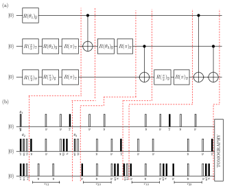
The probabilities can be written as and where , , are the eigenvector of the observables corresponding to Alice, Bob and Charlie, respectively. The observables () , ( are decomposed in terms of linear combinations of Pauli operators and details are given in Appendix-A. The idea is to unitarily map the state to another state , such that where is the observable to be measured in the state and is the z-spin angular momentum of the qubit. This can be achieved by measuring the on the state . For example, one can find the expectation values of and which are involved in the evaluation of probabilities (see Appendix-A), by using the quantum circuit and corresponding NMR pulse sequence given in Fig.5(a) and Fig.5(b) respectively, where the implementation is followed by a measurement of the spin magnetization of the second and third qubits, respectively.

We experimentally calculated the ENC inequalities , and the ENC monogamy relation for the tripartite mixed state given in Eq. (18) for different values of . Experimental values of , , with respect to various values of are plotted in Fig. 6. It can be seen that is violated for the tripartite state with , while is violated for the state with . The monogamy relation is never violated for any value of and the results are in good agreement with the theoretical predictions.

It is seen that the experimental values are always lower than the corresponding theoretical values. This is due to the fact that the maximum value of the inequality is always achieved for a pure state and any addition of noise makes it a mixed state. Therefore, the value is always observed to be lower than the theoretical one. The difference between them also increases with increasing values of upto . For this region, the state prepared for is the dominant one which is shown to violate . Furthermore, the corresponding inequalities are logarithmic in nature, which also compounds the errors for states till . However, after this value the state prepared for dominates and the errors again follow a similar trend. It should be noted that the experimental curve follows the same trend as the theoretical curve.
III.2 Implementation using a pure tripartite state
In this subsection, we experimentally test the monogamy relation Eq. (17) for a pure tripartite state, having two parameters which we can vary. We show that the monogamy relation holds and is in good agreement with theoretical predictions.
We take a pure tripartite state of the form,
| (22) |
where is the normalization factor. We experimentally prepared five different states corresponding to various values of and . The quantum circuit and the corresponding NMR pulse sequence is given in Fig. 7(a), (b). Different pure states corresponding to various values of and were generated by suitably choosing the values of and . Tomograph of one such experimentally prepared state with and is depicted in Fig. 8, with an experimental state fidelity of . After preparing the states, we measured the desired probabilities by mapping the state onto the Pauli basis operators in order to calculate the entropies involved in the inequality Eq. (17) as discussed earlier in Sec. III.1.

We experimentally evaluate , and with respect to the different values of and and the results are given in Table-1. We see that the inequality is violated for and and is violated for and , while the monogamy relationship is never violated for any value of and . This shows that the monogamy relation between the ENC inequalities is obeyed for all such possible states.
| Theory | Experiment | Theory | Experiment | Theory | Experiment | ||
|---|---|---|---|---|---|---|---|
| 1.00 | 0.00 | 0.236 | 0.1560.032 | -1.436 | -1.5220.035 | -1.200 | -1.3660.034 |
| 0.50 | 0.25 | -0.492 | -0.6060.021 | -1.338 | -1.4130.027 | -1.830 | -2.0190.024 |
| 0.50 | 0.50 | -1.017 | -1.1030.022 | -1.017 | -1.0820.030 | -2.034 | -2.1850.026 |
| 0.25 | 0.50 | -1.338 | -1.3970.021 | -0.492 | -0.5980.024 | -1.830 | -1.9950.023 |
| 0.00 | 1.00 | -1.436 | -1.5230.028 | 0.236 | 0.1490.025 | -1.200 | -1.3740.027 |
IV Concluding Remarks
In this paper we develop a theoretical framework to analyze when a scenario will exhibit a monogamous relationship. We perform our analysis of the monogamy relations expected in a general tripartite scenario for the entropic Bell-CHSH inequality and give the first theoretical study of the monogamy of entropic inequalities based on the graph theoretic formalism. We also give the first experimental demonstration of monogamy of entropic correlations using three NMR qubits. Evaluating entropy on an NMR quantum processor is quite hard and has not been performed earlier. We are able to obtain information about entropies using measurements of only the expectation values of observables. We experimentally show the monogamy of entropic inequality for a pure tripartite state as well as for the mixed state. This indicates with certainty that our formalism holds in general.
It should be noted that due to limitations of access to individual events, the NMR implementation of such scenarios involves use of Born rule to interpret the results of measurements. This is not the ideal way of carrying out such experiments and a more refined test would evaluate the requisite probabilities without assuming the Born rule. This is possible on optical systems Zhan et al. (2017); Qu et al. (2020), where the probabilities are calculated by estimating the frequency clicks of the photodetectors rather than the Born rule.
The experimental implementation of monogamy inequalities is important for quantum information processing tasks and our results are a step forward in this direction.
Acknowledgements.
All the experiments were performed on a Bruker Avance-III 600 MHz FT-NMR spectrometer at the NMR Research Facility of IISER Mohali. A. acknowledges financial support from DST/ICPS/QuST/Theme-1/2019/Q-68. K .D. acknowledges financial support from DST/ICPS/QuST/Theme-2/2019/Q-74. JS acknowledges support by Universidad de Sevilla Project Qdisc (Project No. US-15097), with FEDER funds, MCINN/AEI Projet No. PID2020-113738GB-I00, and QuantERA grant SECRET, by MCINN/AEI (Project No. PCI2019-111885-2).Appendix A Observable decomposition in terms of Pauli operators
To experimentally test the inequality on an NMR quantum processor, we have calculated the entropies involved in the inequality by measuring the probabilities for an experimentally prepared state. This can be achieved by decomposing the projectors as linear combinations of Pauli operators, which can then be mapped to a single-qubit Pauli operator. In the tripartite scenario, the probabilities can be written as and for the Alice-Bob and Alice-Charlie entropic CHSH inequalities. To test the monogamy inequality Eq.(17), we measure the probabilities to calculate the entropies involved in the inequalities and .
Probabilities are calculated by decomposing the observables in terms of linear combination of Pauli operators as:
| P(A) | (23) | |||
| P(B) | ||||
| P(A, B) | ||||
| P(A, B) | ||||
| P(A, B) | ||||
| P(A, B) | ||||
| P(A, B) | ||||
| P(A, B) | ||||
| P(A, B) | ||||
| P(A, B) | ||||
| P(B, A) | (24) | |||
| P(B, A) | ||||
| P(B, A) | ||||
| P(B, A) | ||||
| P(A, B) | (25) | |||
| P(A, B) | ||||
| P(A, B) | ||||
| P(A, B) | ||||
| P(A) | (26) | |||
| P(E) | ||||
| P(A, E) | ||||
| P(A, E) | ||||
| P(A, E) | ||||
| P(A, E) | ||||
| P(A, E) | ||||
| P(A, E) | ||||
| P(A, E) | ||||
| P(A, E) | ||||
| P(E, A) | (27) | |||
| P(E, A) | ||||
| P(E, A) | ||||
| P(E, A) | ||||
| P(A, E) | (28) | |||
| P(A, E) | ||||
| P(A, E) | ||||
| P(A, E) | ||||
where with are the Pauli operators. The order of is in the four-base subscript and the base-four notation, 0, 1, 2, 3 can be directly mapped to either identity or Pauli , , and matrices. For example has the form where are identity and Pauli matrices, respectively. Similarly we can find the forms of other (details are given in Singh et al. (2018)).
References
- Brunner et al. (2014) N. Brunner, D. Cavalcanti, S. Pironio, V. Scarani, and S. Wehner, Rev. Mod. Phys. 86, 419 (2014).
- Clauser et al. (1969) J. F. Clauser, M. A. Horne, A. Shimony, and R. A. Holt, Phys. Rev. Lett. 23, 880 (1969).
- BELL (1966) J. S. BELL, Rev. Mod. Phys. 38, 447 (1966).
- Collins et al. (2002) D. Collins, N. Gisin, N. Linden, S. Massar, and S. Popescu, Phys. Rev. Lett. 88, 040404 (2002).
- Kochen and Specker (1975) S. Kochen and E. P. Specker, “The problem of hidden variables in quantum mechanics,” in The Logico-Algebraic Approach to Quantum Mechanics: Volume I: Historical Evolution, edited by C. A. Hooker (Springer Netherlands, Dordrecht, 1975) pp. 293–328.
- Acín et al. (2015) A. Acín, T. Fritz, A. Leverrier, and A. B. Sainz, Communications in Mathematical Physics 334, 533 (2015).
- Araújo et al. (2013) M. Araújo, M. T. Quintino, C. Budroni, M. T. Cunha, and A. Cabello, Phys. Rev. A 88, 022118 (2013).
- Amaral et al. (2014) B. Amaral, M. T. Cunha, and A. Cabello, Phys. Rev. A 89, 030101 (2014).
- Cabello et al. (2014a) A. Cabello, S. Severini, and A. Winter, Phys. Rev. Lett. 112, 040401 (2014a).
- Larsson et al. (2014) J.-A. Larsson, M. Giustina, J. Kofler, B. Wittmann, R. Ursin, and S. Ramelow, Phys. Rev. A 90, 032107 (2014).
- Giustina et al. (2015) M. Giustina, M. A. M. Versteegh, S. Wengerowsky, J. Handsteiner, A. Hochrainer, K. Phelan, F. Steinlechner, J. Kofler, J.-A. Larsson, C. Abellán, W. Amaya, V. Pruneri, M. W. Mitchell, J. Beyer, T. Gerrits, A. E. Lita, L. K. Shalm, S. W. Nam, T. Scheidl, R. Ursin, B. Wittmann, and A. Zeilinger, Phys. Rev. Lett. 115, 250401 (2015).
- Shalm et al. (2015) L. K. Shalm, E. Meyer-Scott, B. G. Christensen, P. Bierhorst, M. A. Wayne, M. J. Stevens, T. Gerrits, S. Glancy, D. R. Hamel, M. S. Allman, K. J. Coakley, S. D. Dyer, C. Hodge, A. E. Lita, V. B. Verma, C. Lambrocco, E. Tortorici, A. L. Migdall, Y. Zhang, D. R. Kumor, W. H. Farr, F. Marsili, M. D. Shaw, J. A. Stern, C. Abellán, W. Amaya, V. Pruneri, T. Jennewein, M. W. Mitchell, P. G. Kwiat, J. C. Bienfang, R. P. Mirin, E. Knill, and S. W. Nam, Phys. Rev. Lett. 115, 250402 (2015).
- Dogra et al. (2016) S. Dogra, K. Dorai, and Arvind, Physics Letters A 380, 1941 (2016).
- Kirchmair et al. (2009) G. Kirchmair, F. Zähringer, R. Gerritsma, M. Kleinmann, O. Gühne, A. Cabello, R. Blatt, and C. F. Roos, Nature 460, 494 EP (2009).
- Klyachko et al. (2008) A. A. Klyachko, M. A. Can, S. Binicioğlu, and A. S. Shumovsky, Phys. Rev. Lett. 101, 020403 (2008).
- Popescu and Rohrlich (1992) S. Popescu and D. Rohrlich, Physics Letters A 169, 411 (1992).
- Braunstein et al. (1992) S. L. Braunstein, A. Mann, and M. Revzen, Phys. Rev. Lett. 68, 3259 (1992).
- Diamanti et al. (2016) E. Diamanti, H.-K. Lo, B. Qi, and Z. Yuan, Npj Quantum Information 2, 16025 EP (2016).
- Scarani et al. (2009) V. Scarani, H. Bechmann-Pasquinucci, N. J. Cerf, M. Dušek, N. Lütkenhaus, and M. Peev, Rev. Mod. Phys. 81, 1301 (2009).
- Acín et al. (2006a) A. Acín, N. Gisin, and L. Masanes, Phys. Rev. Lett. 97, 120405 (2006a).
- Vazirani and Vidick (2014) U. Vazirani and T. Vidick, Phys. Rev. Lett. 113, 140501 (2014).
- Acín and Masanes (2016) A. Acín and L. Masanes, Nature 540, 213 EP (2016).
- Acín et al. (2006b) A. Acín, N. Gisin, and L. Masanes, Phys. Rev. Lett. 97, 120405 (2006b).
- Pawłowski (2010) M. Pawłowski, Phys. Rev. A 82, 032313 (2010).
- Saha and Ramanathan (2017) D. Saha and R. Ramanathan, Phys. Rev. A 95, 030104 (2017).
- Li et al. (2018) T. Li, X. Zhang, Q. Zeng, B. Wang, and X. Zhang, Opt. Express 26, 11959 (2018).
- Pawłowski and Brukner (2009) M. Pawłowski and i. c. v. Brukner, Phys. Rev. Lett. 102, 030403 (2009).
- Ramanathan et al. (2012) R. Ramanathan, A. Soeda, P. Kurzyński, and D. Kaszlikowski, Phys. Rev. Lett. 109, 050404 (2012).
- Kurzyński et al. (2014) P. Kurzyński, A. Cabello, and D. Kaszlikowski, Phys. Rev. Lett. 112, 100401 (2014).
- Zhan et al. (2016) X. Zhan, X. Zhang, J. Li, Y. Zhang, B. C. Sanders, and P. Xue, Phys. Rev. Lett. 116, 090401 (2016).
- Braunstein and Caves (1988) S. L. Braunstein and C. M. Caves, Phys. Rev. Lett. 61, 662 (1988).
- Chaves and Budroni (2016) R. Chaves and C. Budroni, Phys. Rev. Lett. 116, 240501 (2016).
- Chaves (2013) R. Chaves, Phys. Rev. A 87, 022102 (2013).
- Chaves and Fritz (2012) R. Chaves and T. Fritz, Phys. Rev. A 85, 032113 (2012).
- Cao et al. (2016a) L.-Z. Cao, J.-Q. Zhao, X. Liu, Y. Yang, Y.-D. Li, X.-Q. Wang, Z.-B. Chen, and H.-X. Lu, Scientific Reports 6, 23758 EP (2016a).
- Katiyar et al. (2013) H. Katiyar, A. Shukla, K. R. K. Rao, and T. S. Mahesh, Phys. Rev. A 87, 052102 (2013).
- Cao et al. (2016b) L.-Z. Cao, J.-Q. Zhao, X. Liu, Y. Yang, Y.-D. Li, X.-Q. Wang, Z.-B. Chen, and H.-X. Lu, Scientific Reports 6, 23758 (2016b).
- Zhan et al. (2017) X. Zhan, P. Kurzyński, D. Kaszlikowski, K. Wang, Z. Bian, Y. Zhang, and P. Xue, Phys. Rev. Lett. 119, 220403 (2017).
- Qu et al. (2020) D. Qu, P. Kurzyński, D. Kaszlikowski, S. Raeisi, L. Xiao, K. Wang, X. Zhan, and P. Xue, Phys. Rev. A 101, 060101 (2020).
- Kurzyński and Kaszlikowski (2014) P. Kurzyński and D. Kaszlikowski, Phys. Rev. A 89, 012103 (2014).
- Cabello et al. (2014b) A. Cabello, S. Severini, and A. Winter, Phys. Rev. Lett. 112, 040401 (2014b).
- Kurzyński et al. (2012) P. Kurzyński, R. Ramanathan, and D. Kaszlikowski, Phys. Rev. Lett. 109, 020404 (2012).
- Mitra et al. (2007) A. Mitra, K. Sivapriya, and A. Kumar, J. Magn. Reson. 187, 306—313 (2007).
- Gaikwad et al. (2021) A. Gaikwad, Arvind, and K. Dorai, Quantum Information Processing 20, 19 (2021).
- Oliveira et al. (2007) I. S. Oliveira, T. J. Bonagamba, R. S. Sarthour, J. C. C. Freitas, and E. R. deAzevedo, NMR Quantum Information Processing (Elsevier, Linacre House, Jordan Hill, Oxford OX2 8DP, UK, 2007).
- Knill et al. (1998) E. Knill, I. Chuang, and R. Laflamme, Phys. Rev. A 57, 3348 (1998).
- Singh et al. (2019a) A. Singh, A. Gautam, Arvind, and K. Dorai, Physics Letters A 383, 1549 (2019a).
- Singh et al. (2019b) D. Singh, J. Singh, K. Dorai, and Arvind, Phys. Rev. A 100, 022109 (2019b).
- Singh et al. (2018) A. Singh, H. Singh, K. Dorai, and Arvind, Phys. Rev. A 98, 032301 (2018).